
Asymmetry Evolvement and Controllability of a Symmetric Hyperchaotic Map


1
Jiangsu Collaborative Innovation Center of Atmospheric Environment and Equipment Technology (CICAEET), Nanjing University of Information Science & Technology, Nanjing 210044, China
2
School of Artificial Intelligence, Nanjing University of Information Science & Technology, Nanjing 210044, China
3
School of Mathematics and Statistics, Yancheng Teachers University, Yancheng 224002, China
4
Collaborative Innovation Center of Memristive Computing Application (CICMCA), Qilu Institute of Technology, Jinan 250200, China
*
Author to whom correspondence should be addressed.
Symmetry 2021, 13(6), 1039; https://doi.org/10.3390/sym13061039
Submission received: 26 April 2021
/
Revised: 21 May 2021
/
Accepted: 2 June 2021
/
Published: 9 June 2021
(This article belongs to the Special Issue Chaotic Systems and Nonlinear Dynamics)
Abstract
:Trigonometric functions were used to construct a 2-D symmetrical hyperchaotic map with infinitely many attractors. The regime of multistability depends on the periodicity of the trigonometric function, which is closely related to the initial condition. For this trigonometric nonlinearity and the introduction of an offset controller, the initial condition triggers a specific multistability evolvement, in which infinitely countless symmetric and asymmetric attractors are produced. Initial condition-triggered offset boosting is explored, combined with constant controlled offset regulation. Furthermore, this symmetric map gives the sequences in various types of asymmetric attractors, in which the polarity balance is maintained by the initial condition and a negative coefficient due to the trigonometric function. Finally, as determined through the hardware implementation of STM32, the corresponding results agree with the numerical simulation.
1. Introduction
Multistability [1,2,3,4,5,6,7,8,9,10,11] exists widely in continuous systems and discrete systems, in which flexible initial conditions can access different states, resulting in much uncertainty but convenience for chaos applications. Coexisting attractors have numerous manifestations. For example, in a four-dimensional non-autonomous system, the coexisting attractors evolve according to the sign function or with the equilibrium points [12,13]. In three-dimensional continuous systems, the absolute value function can result in offset boosting, inducing the desired distribution of coexisting attractors in phase space [14,15,16]. In fact, an attractor can obtain full control, including the offset in any dimension [17], although under certain conditions coexisting attractors appear in the regime of homogeneous multistablity [18]. In this case, the complex chaotic sequence flexibly switches between unipolar or bipolar, which makes it more applicable in image encryption [19,20,21,22,23,24]. It is well known that some asymmetrical systems have symmetric pairs of attractors when they are of conditional symmetry; meanwhile, some symmetric systems have a pair of coexisting attractors [25,26,27,28,29] when the symmetry is broken. However, symmetrical hyperchaotic maps with asymmetrical chaotic and hyperchaotic attractors are rarely reported. Therefore, it is of great significance to construct a new type of hyperchaotic map for such observations.
In this paper, we propose a new type of 2-D symmetric hyperchaotic map, revealing its special phenomenon of symmetrical coexistence. We also discuss offset boosting. The proposed system is discussed as follows. The mathematical model of the 2-D symmetric hyperchaotic map is presented in Section 2; the basic dynamic behavior of the bifurcation is explored in Section 3; the special multistability phenomenon is discussed in Section 4. Through the reversal of polarity, the abundance of symmetrical coexisting strange attractors is outlined in Section 5. The discussion of offset boosting further illustrates the dynamic behavior of the system in Section 6. Our findings were verified by physical experiments, based on STM32 hardware, and these are presented in Section 7. In the last section, conclusions and discussions are provided.
2. Symmetric Hyperchaotic Map
2.1. Symmetric Hyperchaotic Map Model
Inspired by continuous systems [30] and differently from other discrete maps, but rather by introducing single sinusoidal functions, we propose a novel 2-D discrete map with a simple symmetrical structure. The period is controlled by the parameter a, whereas the parameter b is used as an extra control; the mathematical model is:
The constructed hyperchaotic map has complex dynamics, owing to the sinusoidal function, and shows rich dynamics. Here, m is a natural number (0, 1, 2, 3...), and represent the m-th state, and a and b are the system parameters.
2.2. Fixed Point Analysis
The stability of a discrete map is usually characterized by fixed points. The fixed point satisfies the following equation:
If , we obtain:
Furthermore, we obtain:
Combining (3) and (4), we obtain:
Equation (5) yields four sets of fixed points; two groups of typical fixed points are listed:
where a is a constant, and the Jacobian matrix corresponding to Equation (2) is:
Substituting Equation (6) into Equation (8), when , we can obtain:
There are two eigenvalues, given as:
For or , eigenvalues and , and the fixed point exhibits instability in one or two directions. For , eigenvalues , and , and the fixed point is stable. For the parameter a in the range of , map (1) is dissipative.
Substituting (7) into Equation (8), when and , we can obtain:
For the two eigenvalues of Equation (13): for the cases of and , and , and , the above map gets repelled by the unstable fixed point, leading to an unstable state. However, for the case of , , the two eigenvalues are both in the unit circle, indicating a stable state, which means that the above map is stable for the existence of a stable fixed point. When , the map (1) is dissipative.
In a word, both the location of fixed points and the eigenvalues depend on the coefficient a. A stable or unstable fixed-point affects the dynamics of the map, resulting in different types of attractors.
3. Analysis of Bifurcation Behavior
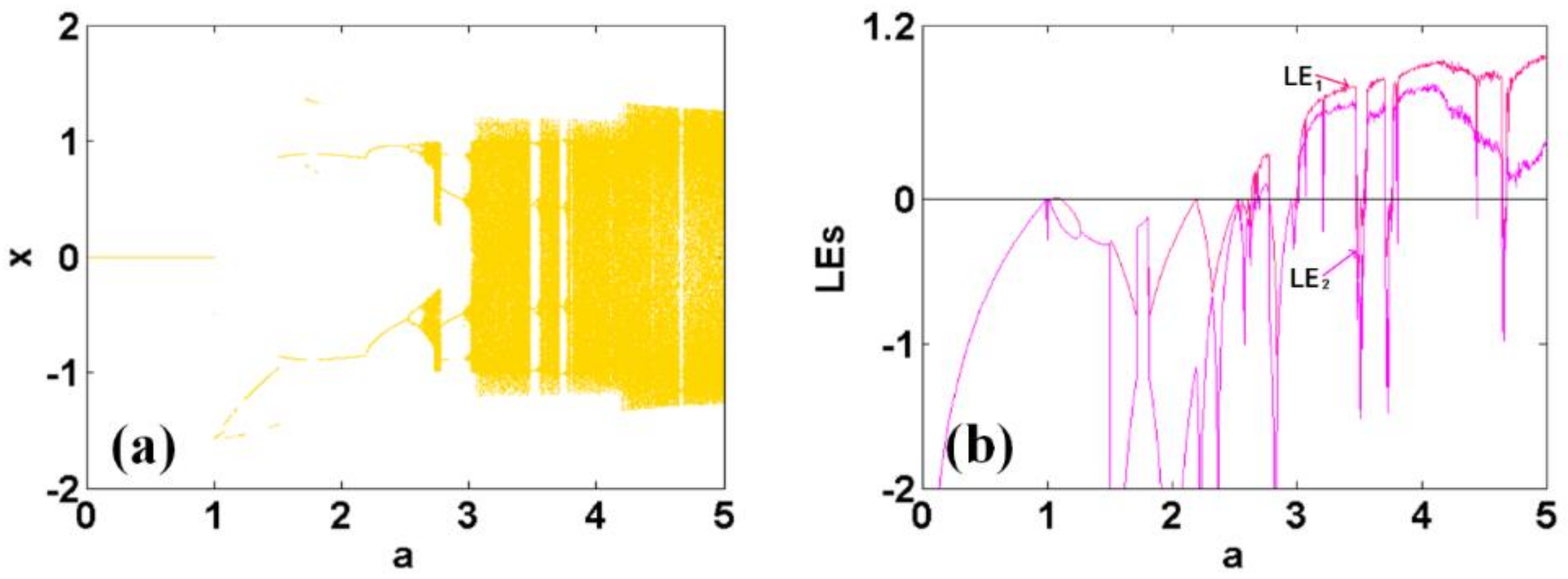
According to the changing of parameter a under the parameter b = 1, we can explore the evolution of the dynamic behavior of the hyperchaotic map as follows. Setting the initial conditions , let a change in the range of [0, 5]; the bifurcation diagram of state variables x, y and corresponding Lyapunov exponents are shown in Figure 1. In the bifurcation diagram shown in Figure 1a, we can see that the map exhibits broken symmetry. When a is located in [3.01, 3.213] [3.217, 3.479], the map enters into chaos and hyperchaos. There is a narrow period window where a is in the gap of [3.213, 3.217], which blocks chaos and hyperchaos, even though the system finally enters hyperchaos. In Figure 2, an asymmetric attractor gradually evolves into hyperchaos with a symmetrical structure under the change of parameter a. In addition, when exploring the dynamics under the parameter b = 0.5 while a varies in the range of [0, 5], map (1) shows its abundant dynamics, with period doubling bifurcation at a deep-breath-like pace. One period doubling process leads to chaos, whereas the other leads to hyperchaos. Symmetry breaking happens again. As shown in Figure 3, it seems that map (1) repeats its dynamics when a changes in the regions of [3.38, 4.05] and [4.29, 5]. Figure 4 shows four types of typical attractors. Table 1 gives the detailed information on these oscillations through Wolf algorithm and Kaplan-Yorke algorithm observations.
4. Multistability Analysis
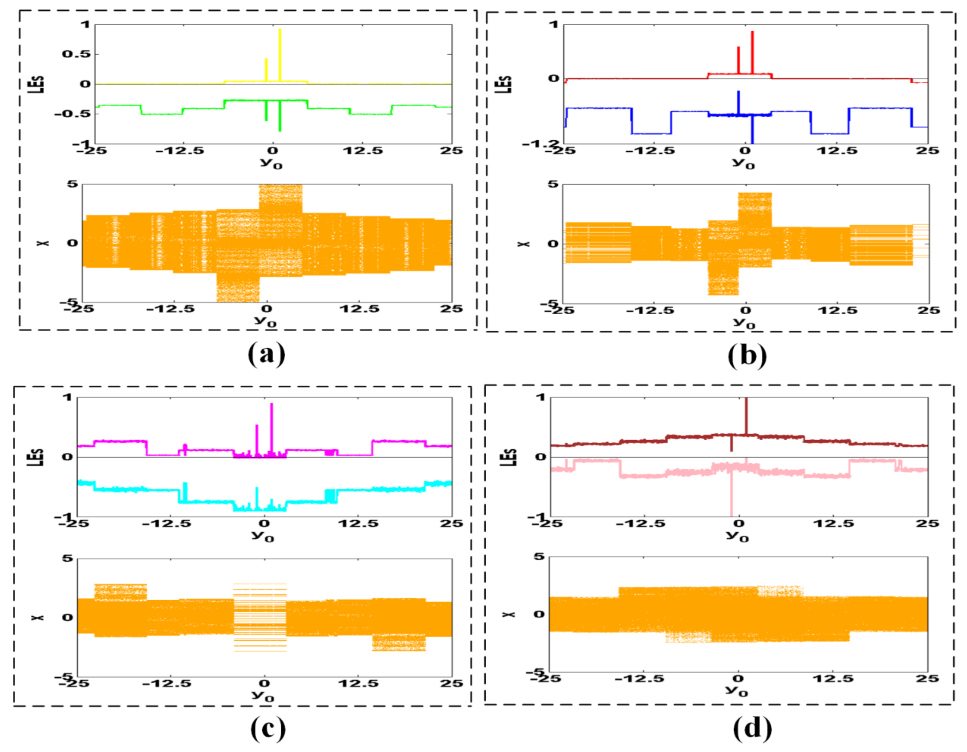
The above hyperchaotic map (1) shows abundant multistability due to the periodic sinusoidal functions. Figure 5 shows the bifurcation dynamics and the corresponding Lyapunov exponents of hyperchaotic map (1) according to the initial state. When the initial value y0 varies in [−25, 25], map (1) switches its oscillation from period to chaos. Specifically, when b = 0.5, even under the same parameters as those of a, system (1) produces different states according to the initial condition of y0.
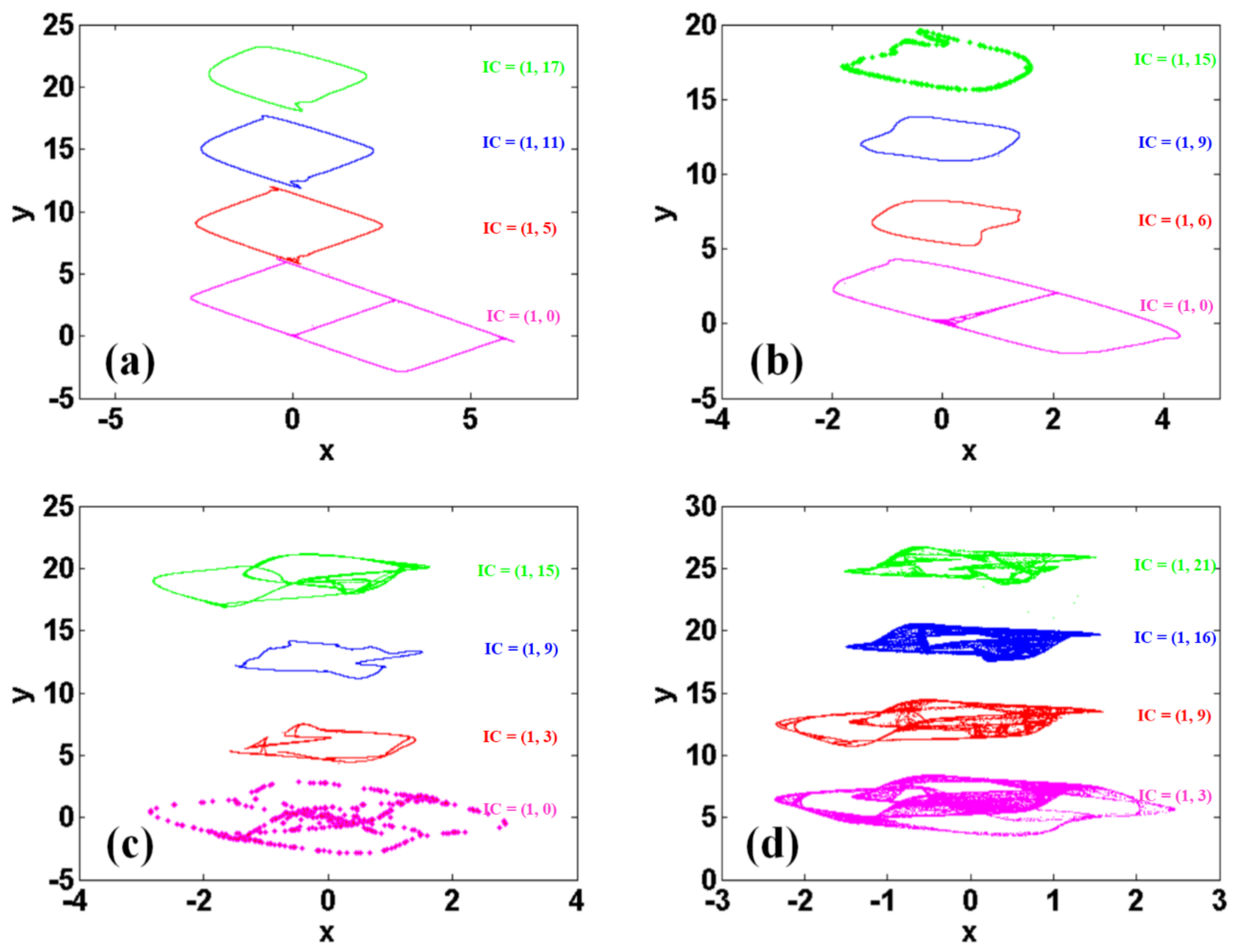
Case 1: When a = 1.041, and the initial conditions (ICs) equal , , , and separately, and system (1) gives two types of coexisting attractors, which are chaos (magenta), quasi-period (red), quasi-period (blue), and quasi-period (green) attractors, accordingly, as shown in Figure 6a.
Case 2: When a = 1.3, the initial conditions (ICs) are respectively , , , and , and the system (1) has three types of coexisting attractors, including chaos (magenta), quasi-period (red), quasi-period (blue), and periodic points (green), as shown in Figure 6b.
Case 3: When a = 1.705, the initial conditions (ICs) are followed by , , , and , the system (1) has two types of coexisting attractors, namely, periodic points (magenta) and chaos (red), chaos (blue), and chaos (blue) attractors, as shown in Figure 6c.
Case 4: When a = 2.1, the order of initial conditions (IC) is , , , and , and the system (1) has multiple chaotic coexisting attractors, such as chaos (magenta), chaos (red), chaos (blue), and chaos (green) attractors, as shown in Figure 6d.
In order to distinguish attractors more clearly, magenta, red, blue and green were selected to represent attractors under different initial conditions.
5. Polarity Control of Symmetrical Attractors
In the symmetrical hyperchaotic map (1), symmetrical attractors can be extracted by means of three approaches. Case 1: system structure-induced symmetrical attractor: map (1) shares a unique symmetrical structure, which can give birth to a symmetrical attractor. Case 2: parameter-induced symmetrical attractor: when , and , the polarity in map (1) is maintained and map (1) gives a pair of symmetrical attractors. Case 3: a coexisting symmetrical pair of attractors: map (1) also has a solution with an asymmetric structure, but the property of symmetry can also bring a new coexisting attractor as the symmetrical pair. In this case, two coexisting attractors can be visited by two sets of initial conditions. Flexible polarity control adds much more convenience to physical engineering applications, where there exist all kinds of challenges and demanding sequences.
Case 1: The map presents a symmetrical attractor (chaos and hyperchaos) according to its own symmetrical structure. As shown in Figure 7, setting the initial condition , and b = 0.5, with a different parameter a, drives the system to chaos and hyperchaos with a symmetrical structure. As shown in Figure 8, the specific parameter a leads to a symmetrical squid-like attractor of different shapes.
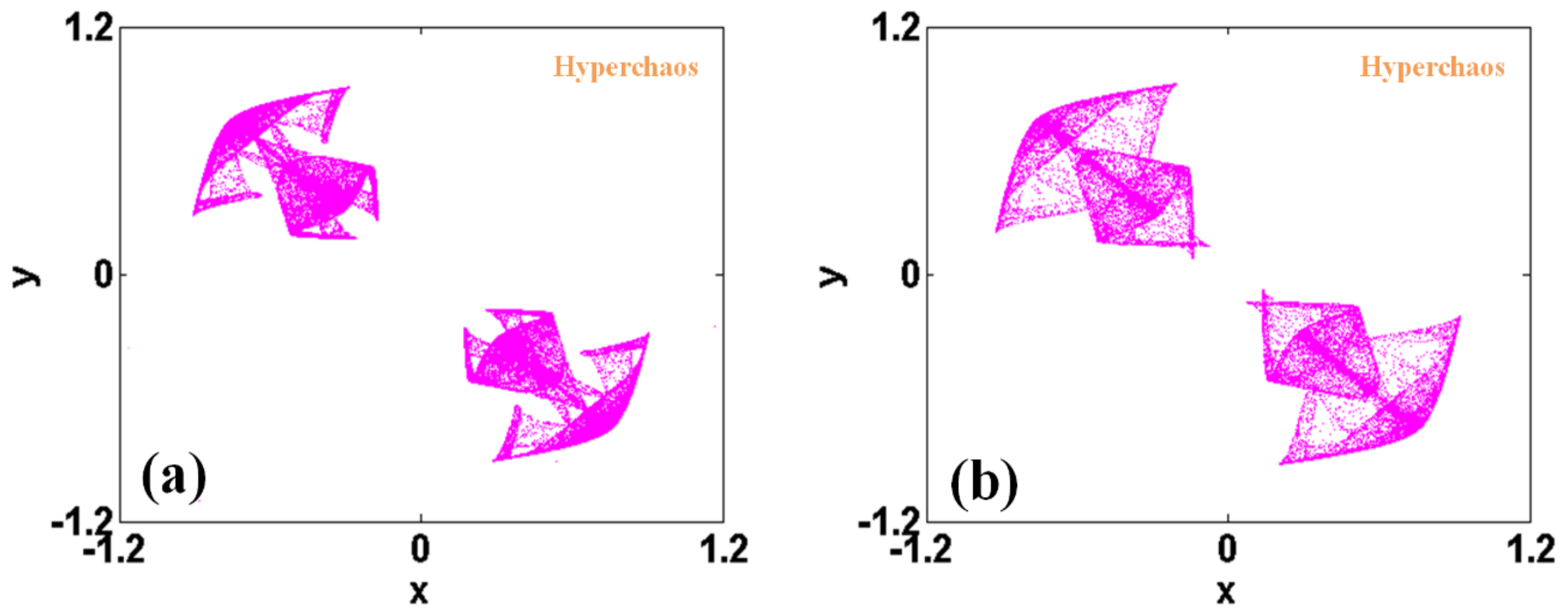
Case 2: Owing to the odd sinusoidal function in the map, the reverse of parameter a can access a new polarity balance through the inverse of variable x, which leads to a reflection symmetry. As shown in Figure 9, when the initial condition and b = 0.5, two groups of attractors with opposite polarity are produced, as shown in Figure 9a,b, respectively. Those hyperchaotic attractors get doubled according to the plane of x = 0.
Case 3: The initial condition can also lead to a symmetrical pair of coexisting attractors for the multistability hidden in the symmetrical map. By reversing the polarity of the initial condition, coexisting attractors with inversion symmetry come out as a pair of chaotic or hyperchaotic attractors. As shown in Figure 10, when b = 0.5, two sets of chaotic and hyperchaotic oscillations are captured by revising the polarity of the initial condition. A basin of attraction for coexisting attractors is identified in Figure 11, in agreement with the symmetrical structure of the system.
6. Offset Boosting
Offset boosting is also an important issue for discrete maps in the control of the polarity of the sequences. However, there are substantial differences between discrete systems and continuous systems in terms of the introduction of offset booster. For discrete systems, an offset booster is usually necessary for both sides, whereas for continuous systems the offset constant is only necessary for the variable on the right-hand side. Here, in particular, let , and hyperchaotic map (1) turns to be:
Although the derived hyperchaotic map (14) has two different periods, namely, and , the parameter c gives a simple control measure for offset boosting. As shown in Figure 12, setting the initial condition , different values of c scatter the controlled phase orbits in the x-dimension. Corresponding discrete sequences with associated offsets are shown on the right side of Figure 12a,b. Adding a constant in the y-dimension can also easily result in offset boosting, which is ignored for the same operation.
7. Hardware Circuit Implementation
In this section, we describe an experiment based on STM32. The corresponding hardware is shown in Figure 13. The numerical calculation was realized using the core board of the single-chip microcomputer STM32F103VE-EK, and the ARM Cortex-M3 is used as the main control chip of the system. The main frequency was set to 72 MHz. The Cortex-M3 kernel supports single cycle multiplication instructions, which satisfies the requirements of floating-point multiplication. The calculation speed was sufficient to implement the chaotic map iterative equation. In addition, we set step 1 for each iteration.
The output was produced by DAC, mainly controlled by the control chip. Two 12-bit digital-to-analog converter modules were used as two independent output signal sources. First, a variable calculation was completed by defining two arrays. Secondly, after initializing the first element of the array, the array elements defined by the discrete equation were updated through each iterative calculation. Each value of the array was amplified so as to be represented as a 12-bit number. Finally, the collected variables were transferred to the control registers of DAC to output the corresponding analog values. As shown in Figure 14, through digital-to-analog conversion, the typical phase trajectories under various parameters were obtained. Figure 15 shows the symmetrical pairs of attractors under the polarity reversal of a. For coexisting attractors, the revision of the polarity of the initial conditions extracts each petal of the attractor, as shown in Figure 16. The results displayed on the oscilloscope, shown in Figure 14, Figure 15 and Figure 16, correspond to those attractors shown in Figure 4, Figure 9 and Figure 10, respectively.
8. Conclusions and Discussion
In this paper, a 2-D hyperchaotic map with a symmetrical structure was constructed by applying trigonometric functions, which exhibited various regimes of multistability. According to the polarity balance induced by the parameters, it can trigger various symmetry evolutions. In some cases, the symmetry is controlled by the initial conditions. Through circuit implementation using STM32, we verified the results of the numerical simulation and the theoretical analysis. In addition, in phase space, the offset boosting has been discussed in detail through linear transformation. In the future, the proposed map could be applied in image encryption, chaotic secure communication, and in other information security applications, in which controlled chaotic and hyperchaotic sequences can be applied as random-like numbers.
Author Contributions
Conceptualization, C.L. and H.J.; Data curation, S.K.; formal analysis, S.K. and Y.W.; funding acquisition, C.L. and Y.Z.; investigation, S.K. and Y.W.; methodology, S.K. and Y.Z.; project administration, C.L. and Y.Z; resources, C.L.; software, S.K.; supervision, C.L., H.J.; validation, S.K.; visualization, S.K.; writing-original draft, S.K.; writing-review and editing, C.L. All authors have read and agreed to the published version of the manuscript.
Funding
This research received no external funding.
Institutional Review Board Statement
Not applicable.
Informed Consent Statement
Not applicable.
Data Availability Statement
The data that support the findings of this study are available from the corresponding author upon reasonable request.
Acknowledgments
This work was supported financially by the National Natural Science Foundation of China (NNSFC) (Grant No. 61871230), the Natural Science Foundation of Jiangsu Province (Grant No. BK20181410) and the Major Program of Natural Science Foundation of Shandong Province (Grant No. ZR2020KA007).
Conflicts of Interest
The authors declare no conflict of interest.
References
- Joshi, A.; Xiao, M. Optical multistability in three-level atoms inside an optical ring cavity. Phys. Rev. Lett. 2003, 91, 143904. [Google Scholar] [CrossRef] [PubMed] [Green Version]
- Jaros, P.; Perlikowski, P.; Kapitaniak, T. Synchronization and multistability in the ring of modified Rössler oscillators. Eur. Phys. J. Spec. Top. 2015, 224, 1541–1552. [Google Scholar] [CrossRef]
- Dudkowski, D.; Jafari, S.; Kapitaniak, T.; Kuznetsov, N.V.; Leonov, G.A.; Prasad, A. Hidden attractors in dynamical systems. Phys. Rep. 2016, 637, 1–50. [Google Scholar] [CrossRef]
- Njitacke, Z.T.; Kengne, J.; Fotsin, H.B.; Negou, A.N.; Tchiotsop, D. Coexistence of multiple attractors and crisis route to chaos in a novel memristive diode bidge-based jerk circuit. Chaos Solitons Fractals 2016, 91, 180–197. [Google Scholar] [CrossRef]
- Kengne, J.; Njitacke, Z.T.; Fotsin, H.B. Dynamical analysis of a simple autonomous jerk system with multiple attractors. Nonlinear Dyn. 2016, 83, 751–765. [Google Scholar] [CrossRef]
- Xu, Q.; Chen, M.; Lin, Y.; Bao, B.C. Multiple attractors in a non-ideal active voltage-controlled memristor based Chua’s circuit. Chaos Solitons Fractals 2016, 83, 186–200. [Google Scholar] [CrossRef]
- Li, C.B.; Sprott, J.C.; Hu, W.; Xu, Y. Infinite multistability in a Self-reproducing Chaotic System. Int. J. Bifurc. Chaos 2017, 27, 1750160. [Google Scholar] [CrossRef]
- Sprott, J.C.; Jafari, S.; Khalaf, A.; Kapitaniak, T. Megastability: Coexistence of a countable infinity of nested attractors in a periodically-forced oscillator with spatially-periodic damping. Eur. Phys. J. Spec. Top. 2017, 226, 1979–1985. [Google Scholar] [CrossRef] [Green Version]
- Bao, B.C.; Li, H.Z.; Zhu, L.; Zhang, X.; Chen, M. Initial-switched boosting bifurcations in 2D hyperchaotic map. Chaos 2020, 30, 033107. [Google Scholar] [CrossRef]
- Bao, H.; Hua, Z.Y.; Wang, N.; Zhu, L.; Chen, M.; Bao, B.C. Initials-boosted Coexisting chaos in a 2D sine map and its hardware implementation. IEEE Trans. Ind. Inform. 2020, 17, 1132–1140. [Google Scholar] [CrossRef]
- Zhang, L.P.; Liu, Y.; Wei, Z.C.; Jiang, H.B.; Bi, Q.S. A novel class of two-dimensional chaotic maps with infinitely many coexisting attractors. Chin. Phys. B 2020, 29, 060501. [Google Scholar] [CrossRef]
- Lai, Q.; Akgul, A.; Zhao, X.W.; Pei, H.Q. Various Types of Coexisting Attractors in a New 4D Autonomous Chaotic System. Int. J. Bifurc. Chaos 2017, 27, 1750142. [Google Scholar] [CrossRef]
- Lai, Q. A Unified Chaotic System with Various Coexisting Attractors. Int. J. Bifurc. Chaos 2021, 31, 2150013. [Google Scholar] [CrossRef]
- Li, C.B.; Sprott, J.C. Variable-boostable chaotic flows. Opt. Int. J. Light Electron Opt. 2016, 127, 10389–10398. [Google Scholar] [CrossRef]
- Sun, W.J.; Zhao, X.T.; Fang, J.; Wang, Y.F. Autonomous memristor chaotic systems of infinite chaotic attractors and circuitry realization. Nonlinear Dyn. 2018, 94, 2879–2887. [Google Scholar] [CrossRef]
- Lai, Q.; Chen, C.Y.; Zhao, X.W.; Kengne, J.; Volos, C. Constructing Chaotic System with Multiple Coexisting Attractors. IEEE Access 2019, 21, 24051–24056. [Google Scholar] [CrossRef]
- Li, C.B.; Lu, T.A.; Chen, G.R.; Xing, H.Y. Doubling the coexisting attractors. Chaos 2019, 29, 051102. [Google Scholar] [CrossRef] [PubMed]
- Li, C.B.; Xu, Y.J.; Chen, G.R.; Liu, Y.J.; Zheng, J.C. Conditional symmetry: Bond for attractor growing. Nonlinear Dyn. 2019, 95, 1245–1256. [Google Scholar] [CrossRef]
- Yang, Y.G.; Guan, B.W.; Li, J.; Li, D.; Zhou, Y.H.; Shi, W.M. Image compression-encryption scheme based on fractional order hyper-chaotic systems combined with 2D compressed sensing and DNA encoding. Opt. Laser Technol. 2019, 119, 105661. [Google Scholar] [CrossRef]
- Yang, F.F.; Mou, J.; Liu, J.; Ma, C.G.; Yan, H.Z. Characteristic analysis of the fractional-order hyperchaotic complex system and its image encryption application. Signal Process. 2020, 169, 107373. [Google Scholar] [CrossRef]
- Ismail, S.M.; Said, L.A.; Radwan, A.G.; Madian, A.H.; Abu-Elyazeed, M.F. A Novel Image Encryption System Merging Fractional-Order Edge Detection and Generalized Chaotic Maps. Signal Process. 2019, 167, 107280. [Google Scholar] [CrossRef]
- Chen, C.; Sun, K.H.; He, S.B. An improved image encryption algorithm with finite computing precision. Signal Process. 2020, 168, 107340. [Google Scholar] [CrossRef]
- Deng, J.; Zhou, M.J.; Wang, C.H.; Xu, C. Image segmentation encryption algorithm with chaotic sequence generation participated by cipher and multi-feedback loops. Multimed. Tools Appl. 2021, 80, 13821–13840. [Google Scholar] [CrossRef]
- Zeng, J.; Wang, C.H. A Novel Hyperchaotic Image Encryption System Based on Particle Swarm Optimization Algorithm and Cellular Automata. Secur. Commun. Netw. 2021, 5, 1–15. [Google Scholar] [CrossRef]
- Wei, Z.; Wang, R.; Liu, A. A new finding of the existence of hidden hyperchaotic attractors with no equilibria. Math. Comput. Simul. 2014, 100, 13–23. [Google Scholar] [CrossRef]
- Jafari, S.; Sprott, J.C.; Nazarimehr, F. Recent new examples of hidden attractors. Eur. Phys. J. Spec. Top. 2015, 224, 1469–1476. [Google Scholar] [CrossRef]
- Bao, B.C.; Li, Q.D.; Wang, N.; Xu, Q. Multistability in Chua’s circuit with two stable node-foci. Chaos 2016, 26, 043111. [Google Scholar] [CrossRef] [PubMed]
- Lai, Q.; Chen, S.M. Research on a new 3D autonomous chaotic system with coexisting attractors. Opt. Int. J. Light Electron Opt. 2017, 127, 3000–3004. [Google Scholar] [CrossRef]
- Chen, M.; Xu, Q.; Lin, Y.; Bao, B.C. Multistability induced by two symmetric stable node-foci in modified canonical Chua’s circuit. Nonlinear Dyn. 2017, 87, 789–802. [Google Scholar] [CrossRef]
- Li, C.B.; Sprott, J.C.; Mei, Y. An infinite 2-D lattice of strange attractors. Nonlinear Dyn. 2017, 89, 2629–2639. [Google Scholar] [CrossRef]
Figure 1.
Dynamic behavior of hyperchaotic map (1) under the initial conditions and parameter b = 1 when a changing in the region of [0, 5]: (a) bifurcation diagram, (b) Lyapunov exponents.
Figure 1.
Dynamic behavior of hyperchaotic map (1) under the initial conditions and parameter b = 1 when a changing in the region of [0, 5]: (a) bifurcation diagram, (b) Lyapunov exponents.

Figure 2.
Typical attractors of hyperchaotic map (1) with b = 1 and initial conditions : (a) a = 2.71, (, ); (b) a = 2.728, (, ); (c) a = 2.74, (, ); (d) a = 2.77, (, ).
Figure 2.
Typical attractors of hyperchaotic map (1) with b = 1 and initial conditions : (a) a = 2.71, (, ); (b) a = 2.728, (, ); (c) a = 2.74, (, ); (d) a = 2.77, (, ).

Figure 3.
When a is in the range of [0, 5], dynamic behavior of hyperchaotic map (1) with b = 0.5 and initial conditions : (a) bifurcation diagram, (b) Lyapunov exponents.
Figure 3.
When a is in the range of [0, 5], dynamic behavior of hyperchaotic map (1) with b = 0.5 and initial conditions : (a) bifurcation diagram, (b) Lyapunov exponents.

Figure 4.
Two typical attractors of map (1) with b = 0.5 and initial conditions : (a) a = 0.76, (, ); (b) a = 1.3, (, ); (c) a = 1.852, (, ); (d) a = 3.11, (, ).
Figure 4.
Two typical attractors of map (1) with b = 0.5 and initial conditions : (a) a = 0.76, (, ); (b) a = 1.3, (, ); (c) a = 1.852, (, ); (d) a = 3.11, (, ).

Figure 5.
Dynamic evolution of map (1) with b = 0.5 under various initial conditions : (a) a = 1.3, (b) a = 1.48, (c) a = 1.705, (d) a = 2.1.
Figure 5.
Dynamic evolution of map (1) with b = 0.5 under various initial conditions : (a) a = 1.3, (b) a = 1.48, (c) a = 1.705, (d) a = 2.1.

Figure 6.
Typical attractors of map (1) with b = 0.5 under various initial conditions : (a) a = 1.3, (b) a = 1.48, (c) a = 1.705, (d) a = 2.1.
Figure 6.
Typical attractors of map (1) with b = 0.5 under various initial conditions : (a) a = 1.3, (b) a = 1.48, (c) a = 1.705, (d) a = 2.1.

Figure 7.
Symmetrical chaotic solutions of map (1) with initial conditions and b = 0.5: (a) a = 1.34, (b) a = 1.56, (c) a = 1.80, (d) a = 2.10.
Figure 7.
Symmetrical chaotic solutions of map (1) with initial conditions and b = 0.5: (a) a = 1.34, (b) a = 1.56, (c) a = 1.80, (d) a = 2.10.

Figure 8.
Symmetrical hyperchaotic solutions of map (1) with initial conditions and b = 0.5: (a) a = 3.11, (b) a = 3.142.
Figure 8.
Symmetrical hyperchaotic solutions of map (1) with initial conditions and b = 0.5: (a) a = 3.11, (b) a = 3.142.

Figure 9.
Coexisting symmetrical hyperchaotic solutions of map (1) with initial conditions and b = 0.5: (a) , (b) .
Figure 9.
Coexisting symmetrical hyperchaotic solutions of map (1) with initial conditions and b = 0.5: (a) , (b) .

Figure 10.
Coexisting symmetrical chaotic solutions of map (1) with b = 0.5 and initial conditions : (a) a = 1.3, (b) a = 3.1.
Figure 10.
Coexisting symmetrical chaotic solutions of map (1) with b = 0.5 and initial conditions : (a) a = 1.3, (b) a = 3.1.

Figure 11.
Basin of attraction for two coexisting symmetrical attractors of map (1), with a = 1.3, b = 0.5.
Figure 11.
Basin of attraction for two coexisting symmetrical attractors of map (1), with a = 1.3, b = 0.5.

Figure 12.
Controlled discrete dynamics with various offsets in map (15) with initial conditions : (a) a = 0.75, b = 0.5 (red: c = 6, green: c = 0, blue: ), (b) a = 3.11, b = 1.55 (magenta: c = 1, cyan: c = 0, orange: ).
Figure 12.
Controlled discrete dynamics with various offsets in map (15) with initial conditions : (a) a = 0.75, b = 0.5 (red: c = 6, green: c = 0, blue: ), (b) a = 3.11, b = 1.55 (magenta: c = 1, cyan: c = 0, orange: ).

Figure 13.
Experimental setup based on STM32 for map (1), with a = 3.11, b = 0.5.

Figure 14.
Typical solutions of map (1) with initial conditions and b = 0.5: (a) a = 0.76, quasi-period; (b) a = 1.300, chaos; (c) a = 1.853, periodic points; (d) a = 3.110, hyperchaos.
Figure 14.
Typical solutions of map (1) with initial conditions and b = 0.5: (a) a = 0.76, quasi-period; (b) a = 1.300, chaos; (c) a = 1.853, periodic points; (d) a = 3.110, hyperchaos.

Figure 15.
Symmetrical hyperchaotic solutions of map (1) with b = 0.5 controlled by a: (a) , (b) .

Figure 16.
Coexisting symmetrical solutions of map (1) with b = 0.5 controlled by initial conditions: (a) a = 1.3, (b) a = 3.1.
Figure 16.
Coexisting symmetrical solutions of map (1) with b = 0.5 controlled by initial conditions: (a) a = 1.3, (b) a = 3.1.


Table 1.
Lyapunov exponents, Kaplan-Yorke dimension of typical attractors in map (1) with b = 0.5.
| Attractor Type | |||
|---|---|---|---|
| 0.76 | 0, −0.3653 | 0 | Quasi-period |
| 1.300 | 0.0847, −0.6667 | 1.127 | Chaos |
| 1.852 | −0.0257, −0.4089 | 0 | Periodic points |
| 3.110 | 0.2121, 0.0985 | 2 | Hyperchaos |
Publisher’s Note: MDPI stays neutral with regard to jurisdictional claims in published maps and institutional affiliations. |
© 2021 by the authors. Licensee MDPI, Basel, Switzerland. This article is an open access article distributed under the terms and conditions of the Creative Commons Attribution (CC BY) license (https://creativecommons.org/licenses/by/4.0/).
Share and Cite
MDPI and ACS Style
Kong, S.; Li, C.; Jiang, H.; Zhao, Y.; Wang, Y. Asymmetry Evolvement and Controllability of a Symmetric Hyperchaotic Map. Symmetry 2021, 13, 1039. https://doi.org/10.3390/sym13061039
AMA Style
Kong S, Li C, Jiang H, Zhao Y, Wang Y. Asymmetry Evolvement and Controllability of a Symmetric Hyperchaotic Map. Symmetry. 2021; 13(6):1039. https://doi.org/10.3390/sym13061039
Chicago/Turabian StyleKong, Sixiao, Chunbiao Li, Haibo Jiang, Yibo Zhao, and Yanling Wang. 2021. "Asymmetry Evolvement and Controllability of a Symmetric Hyperchaotic Map" Symmetry 13, no. 6: 1039. https://doi.org/10.3390/sym13061039
Note that from the first issue of 2016, this journal uses article numbers instead of page numbers. See further details here.