The Properties of a Decile-Based Statistic to Measure Symmetry and Asymmetry


1
Institute of Research and Development, Duy Tan University, Da Nang 550000, Vietnam
2
Department of Statistics, Faculty of Science, Fasa University, Fasa, Fars 7461686131, Iran
3
Department of Mathematics, Faculty of Art and Sciences, Cankaya University, Ankara 06530, Turkey
4
Institute of Space Sciences, 077125 Bucharest, Romania
5
Fractional Calculus, Optimization and Algebra Research Group, Faculty of Mathematics and Statistics, Ton Duc Thang University, Ho Chi Minh City 72915, Vietnam
*
Author to whom correspondence should be addressed.
Symmetry 2020, 12(2), 296; https://doi.org/10.3390/sym12020296
Submission received: 20 January 2020
/
Revised: 1 February 2020
/
Accepted: 4 February 2020
/
Published: 18 February 2020
(This article belongs to the Special Issue Multibody Systems with Flexible Elements)
Abstract
:This paper studies a simple skewness measure to detect symmetry and asymmetry in samples. The statistic can be obviously applied with only three short central tendencies; i.e., the first and ninth deciles, and the median. The strength of the statistic to find symmetry and asymmetry is studied by employing numerous Monte Carlo simulations and is compared with some alternative measures by applying some simulation studies. The results show that the performance of this statistic is generally good in the simulation.
1. Introduction
In scientific studies, the researchers can summarize a given dataset using descriptive statistics. The descriptive statistics contain three known tendencies: central tendencies, dispersion tendencies and shape tendencies [1]. The central and dispersion tendencies, such as mean, median, standard deviation and variance deal with the convenience of the dataset [1,2,3,4,5]. The shape tendencies, such as skewness and kurtosis, are related to the distribution of dataset [6,7,8]. These measures which may be utilized in divergent disciplines consist of the tests of normality and of the lustiness for normal theoretical procedures. Skewness is often utilized to reference to symmetry. Nevertheless, symmetry is not often perspicuously defined, and it is thought that everybody knows it. There are some definitions about symmetry relying on the disciplines that it is utilized in. In literature, any statement related to the symmetry of a structure has to be done with reference to some rules of symmetry—a score, a line or an axis [9]. In the statistical inference, the meaningful score or axis is taken as the center of a distribution. There are several measures employed to quantify the degree of skewness of a distribution. Assume that , , , σ,, and , are the mean; median; mode; standard deviation; third centered moment; and the first and the third quartiles, respectively. The statistics introduced for measuring the skewness are Pearson’s coefficient of skewness:
Pearson’s second coefficient of skewness:
Yule’s coefficient of skewness:
the standardized third central moment:
Bowley’s coefficient of skewness:
and three Galip’s coefficients of skewness:
[9,10,11,12,13,14,15,16,17].
Although there are numerous different measures, and practical elongations of the above coefficients were proposed afterward, the original measures are still employed to this day, especially (or its variants). It is largely utilized in statistical calculation software.
When we face a dataset containing outliers, we need a measure that can carefully consider these outliers. Therefore, probably, the measures that are based on the extreme values (max and min) such as three Galip’s coefficients of skewness; are based on the first and the last quartiles ( and ) such as Bowley’s coefficient of skewness; or are based on the first and the last deciles ( and ), should be more effective than other methods. The previous studies indicated that the three Galip’s coefficients of skewness had the most power to detect symmetry and asymmetry. But the Bowley’s coefficient of skewness acted not so well. There is no deep study about the definition of skewness based on deciles and the comparison between them and other alternatives.
In this work, at first, we consider the definition of skewness based on deciles and then study its asymptotic properties, similar to the approach that was applied in [18,19,20,21,22,23]. Finally, the power of the considered statistic to detect symmetry and asymmetry is compared with the powers of other measures of skewness.
2. Decile-Based Skewness
Let be a sample from a distribution on the real line, and we suppose that is continuous so that all observations are distinct with probability one. We may then arrange the observations in increasing order without ties, . These variables are called the order statistics, where is the kth order statistic. For 0 < p < 1, the th quantile of is defined as and the corresponding sample quantile is defined as where , the ceiling of (the smallest integer greater than or equal to ). Let and be the first and nine sample deciles (0.1 and 0.9 quantiles), respectively. We consider our statistic for measuring the skewness by
In the following, the asymptotic distribution of the proposed statistic is explored.
Lemma 1.
Letbe independent, identically distributed (iid in short) random variables fromand, which are order statistics of. If, then
whereand
Proof.
Assume that are iid exponential variables with mean 1 and . Additionally, assume that , and as , , , and n. Then by the extension of the results given in [24],
such that
Take ; then, by Cramer’s theorem [24],
Finally, the proof is completed with the reality that the distribution of given is the same as the distribution of . □
Corollary 1.
Letbe iid random variables with density and distribution functionsand, respectively. Additionally, assume thatis continuous and positive in a neighborhood of the quantilesandwith; then,
where
Proof.
By applying the transformation to the variables in Lemma 1, the proof will be completed. Be careful that the derivation of is
□
The asymptotic distribution of SK is provided in the following theorem. This is our major contribution. It is also necessary to infer the skewness of population.
Theorem 1.
Letbe iid random variables with density function f. Additionally, assume thatis continuous and positive in a neighborhood of the quantilesand. Then, the asymptotic distribution of the proposed statistic can be illustrated by
where
Proof.
The proof is simply achieved using Cramer’s theorem [24] and taking . □
Corollary 2.
Letbe iid random variables from; then, the asymptotic distribution of the proposed statistic is given by
These results can be employed to build an asymptotical confidence interval and to check the hypothesis.
2.1. Asymptotic Confidence Interval
Now, can be utilized as a pivotal quantity to build a confidence interval asymptotic to a population’s skewness,
where
2.2. Hypothesis Testing
Hypothesis testing related to is a crucial issue in practical application. For instance, the assumption is tantamount to the symmetry. Generally, to test , the test statistic can be
Similar to the methodology provided in Theorem 1, it can prove that with the null hypothesis, has, asymptotically, standard normal distribution.
3. Asymptotic Properties of the Proposed Statistic
In this part, many data sets are drawn to analyze the performance of the proposed approach, for distinct symmetric distributions and divergent sample sizes. Firstly, we checked that the given CI and test statistic are truly the asymptotic CI and test statistic. For every parameter, the experiential coverage probability (percentage of runs for which the given CI contains zero (true skewness)) was calculated by relying on 10,000 repetitions using statistical R 3.6.2 and SPSS 25 software. In addition, for each repetition, the value of the given test statistic is presented and normal Q–Q plots of the given test statistic are provided. The Shapiro-Wilk’s normality test is used to confirm the normality of the given test statistic. The experiential coverage probabilities for divergent parameters are illustrated as in Table 1.
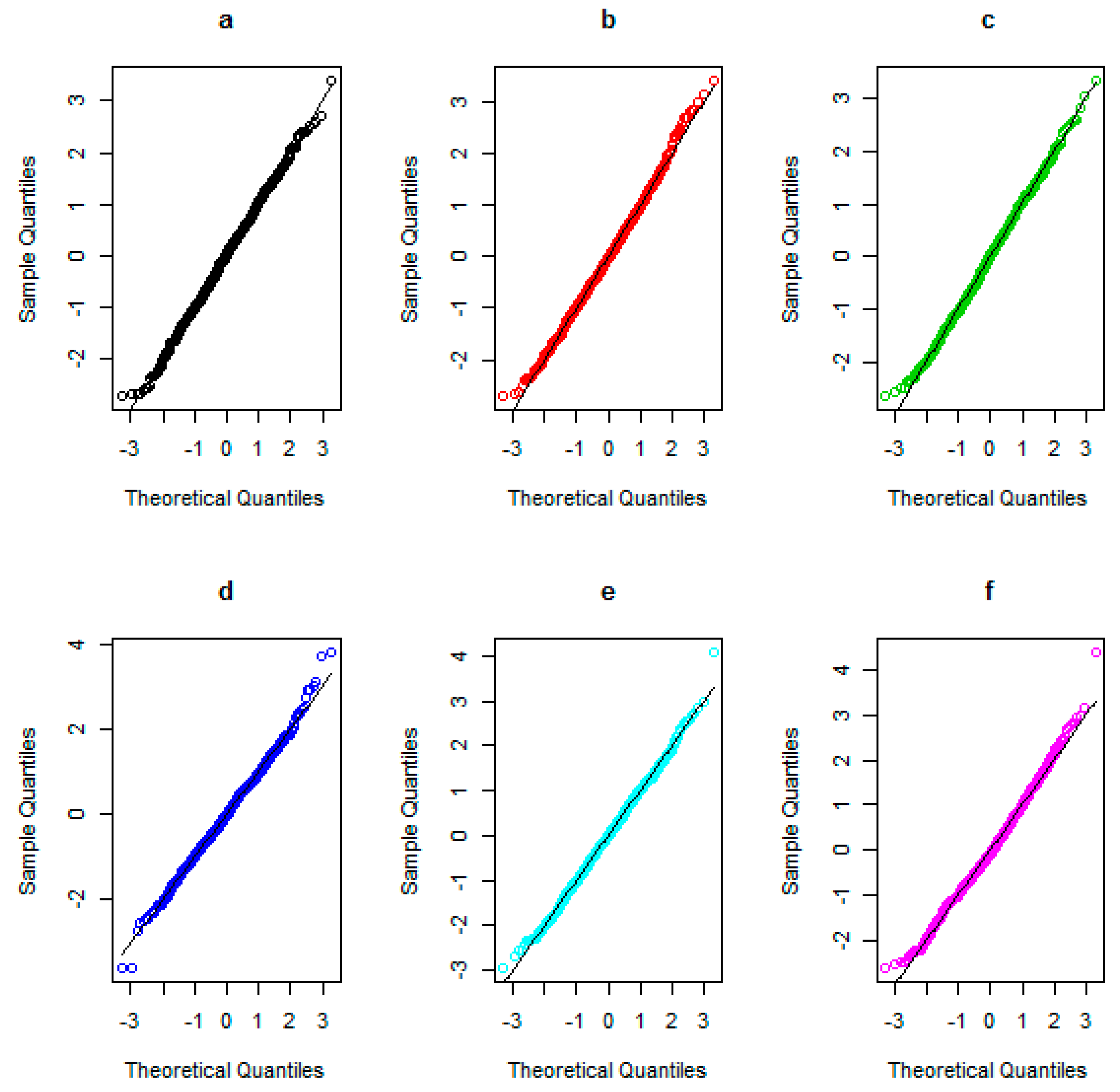
The results show that the experiential coverage probability of proposed approach is more than nominal level (0.95), especially when the sample sizes grow. In the other hand, we can admit the given CI as the asymptotic CI for the skewness of population. Figure 1 and Table 2 show the Q–Q plots for the standard normal distribution and the results of Shapiro-Wilk’s normality test in the test statistic, respectively.
It can be then seen that the asymptotic properties are relatively satisfied in all situations (p-value is greater than 5%). Thereafter, it can be seen that our approach is a good choice to build a CI and execute hypothesis testing for the skewness of a population.
4. Comparison with Alternative Measures
To check the performances of the considered statistic, its power to detect asymmetry is compared with the conventional measures of skewness by employing a Monte Carlo simulation. As in Section 3, numerous data sets were drawn to check the performances of the measures, for different asymmetric distributions and different sample sizes using R software. For this purpose, we generated 10,000 samples of size from a chi-square distribution with m degrees of freedom, . We considered three cases: extremely skewed (m = 1), moderately skewed (m = 5) and slightly skewed (m = 40). The powers (at 5% significant level) of different measures to detect asymmetry are summarized in Table 3.
As preliminary results, based on the maximum power, it can be observed that the performances of , and are approximately similar and are more powerful than other methods for all simulated datasets, and are therefore are very promising. The performances of and are approximately similar and have the next best ranks, while has the worst performance in all situations. In general, the measures that are based on the extreme values (maximum and minimum), such as three Galip’s coefficients of skewness, and those based on the first and the last deciles ( and ), are more effective than other methods, because of their better performances and easy calculations.
5. Discussion
In this work, at first, we considered the definition of skewness based on deciles, and then studied its asymptotic properties. The results showed that the experiential coverage probability of this measure was more than nominal level (0.95), especially when the sample size was increased. The Q–Q plots versus the standard normal distribution and the results of Shapiro-Wilk’s normality test verified the theoretical asymptotic properties. Finally, the power of the considered statistic to detect symmetry and asymmetry was compared with the powers of other measures of skewness. The power study indicated that the performances of decile-based measure and three Galip’s coefficients of skewness were approximately similar, and were more powerful than other methods for all simulated datasets, and are therefore are promising for application in practice.
6. Conclusions
We presented a simple measure to find skewness in patterns. The new measure relies on a new definition of skewness that contains many outstanding advantages. The proposed coefficient of skewness could be obviously calculated with only three short statistics; i.e., the first and nine deacons and the median. The strength of the proposed statistic to find symmetry and asymmetry was studied by employing numerous Monte Carlo simulations. The results show that the performance of new statistic is generally very good in the simulation. There are many definitions to describe symmetry and asymmetry. To investigate the skewness in datasets including outliers, we should use the measures that consider the effects of outliers. Therefore, probably, the measures that are based on the extreme values (maximum and minimum), such as three Galip’s coefficients of skewness; those based on the first and the last quartiles ( and ), such as Bowley’s coefficient of skewness; and those based on the first and the last deciles ( and ), are candidates for application. Other studies showed that Galip’s coefficients of skewness are more powerful for detecting symmetry and asymmetry. There is no deep study about the definition of skewness based on deciles and a comparison between them and other alternatives. In this work, at first, we considered the definition of skewness based on deciles and then studied its asymptotic properties. Finally, the power of the considered statistic to detect symmetry and asymmetry was compared with the powers of other measures of skewness. For future works, we suggest readers to use a definition of skewness based on combinations of more deciles, not only the first and the ninth deciles. We think this combination will improve the detection of symmetry and asymmetry.
Author Contributions
Conceptualization, M.R.M., R.N., D.B. and K.-H.P.; data curation, M.R.M.; formal analysis, M.R.M., R.N. and K.-H.P.; investigation, M.R.M., R.N. and D.B.; methodology, M.R.M. and K.-H.P.; project administration, D.B.; supervision, M.R.M.; validation, M.R.M.; visualization, M.R.M.; writing—original draft, M.R.M. and R.N.; writing—review and editing, D.B. and K.-H.P. All authors have read and agreed to the published version of the manuscript.
Funding
This research received no external funding.
Conflicts of Interest
The authors declare no conflict of interest.
References
- Sprinthall, R.C.; Fisk, S.T. Basic Statistical Analysis; Prentice Hall: Englewood Cliffs, NJ, USA, 1990. [Google Scholar]
- Manikandan, S. Measures of central tendency: Median and mode. J. Pharmacol. Pharm. 2011, 2, 214. [Google Scholar] [CrossRef] [Green Version]
- Weisberg, H.; Weisberg, H.F. Central Tendency and Variability; Sage: Thousand Oaks, CA, USA, 1992. [Google Scholar]
- Deshpande, S.; Gogtay, N.J.; Thatte, U.M. Measures of central tendency and dispersion. J. Assoc. Physicians India 2016, 64, 64–66. [Google Scholar]
- Manikandan, S. Measures of dispersion. J. Pharmacol. Pharm. 2011, 2, 315. [Google Scholar] [CrossRef]
- Kim, T.H.; White, H. On more robust estimation of skewness and kurtosis. Financ. Res. Lett. 2004, 1, 56–73. [Google Scholar] [CrossRef]
- Oja, H. On location, scale, skewness and kurtosis of univariate distributions. Scand J. Stat. 1981, 1, 154–168. [Google Scholar]
- Wilkins, J.E. A note on skewness and kurtosis. Ann. Math Stat. 1944, 15, 333–335. [Google Scholar] [CrossRef]
- Murphy, E.A. Skewness and asymmetry of distributions. Metamedicine 1982, 3, 87–99. [Google Scholar] [CrossRef]
- Arnold, B.C.; Groeneveld, R.A. Skewness and kurtosis orderings: An introduction. Lect. Notes Monogr. Ser. 1992, 22, 17–24. [Google Scholar]
- Arnold, B.C.; Groeneveld, R.A. Measuring skewness with respect to the mode. Am. Stat. 1995, 49, 34–38. [Google Scholar]
- Doane, D.P.; Seward, L.E. Measuring Skewness: A Forgotten Statistic? J. Stat. Educ. 2011, 19, 1–18. [Google Scholar] [CrossRef]
- García, V.J.; Martel, M.; Vázquez-Polo, F.J. Complementary information for skewness measures. Stat. Neerl 2015, 69, 442–459. [Google Scholar] [CrossRef]
- Groeneveld, R.A.; Meeden, G. Measuring skewness and kurtosis. Statistician 1984, 33, 391–399. [Google Scholar] [CrossRef]
- Mahmoudi, M.R.; Nasirzadeh, R.; Mohammadi, M. On the Ratio of Two Independent Skewnesses. Commun. Stat. Theory Methods 2019, 48, 1721–1727. [Google Scholar] [CrossRef]
- Tabor, J. Investigating the investigative task: Testing for skewness–An investigation of different test statistics and their power to detect skewness. J. Stat. Educ. 2010, 18, 1–13. [Google Scholar] [CrossRef] [Green Version]
- Tajuddin, I.H. A simple measure of skewness. Stat. Neerl 1996, 50, 362–366. [Google Scholar] [CrossRef]
- Haghbin, H.; Mahmoudi, M.R.; Shishebor, Z. Large Sample Inference on the Ratio of Two Independent. Binomial Proportions. J. Math. Ext. 2011, 5, 87–95. [Google Scholar]
- Mahmoudi, M.R.; Mahmoodi, M. Inferrence on the Ratio of Variances of Two Independent Populations. J. Math. Ext. 2014, 7, 83–91. [Google Scholar]
- Mahmoudi, M.R.; Mahmoodi, M. Inferrence on the Ratio of Correlations of Two Independent Populations. J. Math. Ext. 2014, 7, 71–82. [Google Scholar]
- Mahmouudi, M.R.; Maleki, M.; Pak, A. Testing the Difference between Two Independent Time Series Models. Iran. J. Sci. Technol. Trans. A Sci. 2017, 41, 665–669. [Google Scholar] [CrossRef]
- Mahmoudi, M.R.; Mahmoudi, M.; Nahavandi, E. Testing the Difference between Two Independent Regression Models. Commun. Stat. Theory Methods 2016, 45, 6284–6289. [Google Scholar] [CrossRef]
- Mahmoudi, M.R.; Behboodian, J.; Maleki, M. Large Sample Inference about the Ratio of Means in Two Independent Populations. J. Stat. Theory Appl. 2017, 16, 366–374. [Google Scholar] [CrossRef] [Green Version]
- Ferguson, T.S. A Course in Large Sample Theory; Chapman & Hall: London, UK, 1996. [Google Scholar]
Figure 1.
The Q–Q plots versus standard normal distribution. Normal distribution: (a), (b). t distribution: (c), (d). Uniform distribution: (e), (f).
Figure 1.
The Q–Q plots versus standard normal distribution. Normal distribution: (a), (b). t distribution: (c), (d). Uniform distribution: (e), (f).


Table 1.
The experiential coverage probability of the proposed confidence interval.
| Distribution | ||||||
|---|---|---|---|---|---|---|
| Normal (1,5) | 0.9732 | 0.9734 | 0.9743 | 0.9744 | 0.975 | 0.9761 |
| t(10) | 0.9916 | 0.9928 | 0.9934 | 0.9939 | 0.9942 | 0.9947 |
| U(0,1) | 0.9485 | 0.949 | 0.9491 | 0.9502 | 0.9521 | 0.9569 |
Table 2.
Shapiro-Wilk’s normality test p-value for the given test statistic.
| Distribution | ||||||
|---|---|---|---|---|---|---|
| Normal (1,5) | 0.7131 | 0.7174 | 0.7899 | 0.8436 | 0.9077 | 0.9213 |
| t(10) | 0.433 | 0.6515 | 0.781 | 0.8317 | 0.9603 | 0.9945 |
| U(0,1) | 0.3144 | 0.5566 | 0.6034 | 0.6219 | 0.8249 | 0.9488 |
Table 3.
The powers of different measures to detect skewness.
| Distribution | Measure | n | ||
|---|---|---|---|---|
| 10 | 20 | 50 | ||
| Extremely Skewed | 0.798 | 0.989 | 1.000 | |
| 0.687 | 0.942 | 1.000 | ||
| 0.817 | 0.991 | 1.000 | ||
| 0.834 | 0.992 | 1.000 | ||
| 0.461 | 0.831 | 0.997 | ||
| 0.200 | 0.151 | 0.130 | ||
| 0.616 | 0.869 | 0.999 | ||
| 0.616 | 0.869 | 0.999 | ||
| 0.260 | 0.403 | 0.711 | ||
| Moderately Skewed | 0.318 | 0.597 | 0.945 | |
| 0.297 | 0.530 | 0.889 | ||
| 0.321 | 0.564 | 0.911 | ||
| 0.318 | 0.623 | 0.941 | ||
| 0.145 | 0.397 | 0.814 | ||
| 0.132 | 0.108 | 0.100 | ||
| 0.207 | 0.344 | 0.651 | ||
| 0.207 | 0.344 | 0.651 | ||
| 0.123 | 0.156 | 0.224 | ||
| Slightly Skewed | 0.144 | 0.163 | 0.289 | |
| 0.129 | 0.165 | 0.288 | ||
| 0.135 | 0.175 | 0.284 | ||
| 0.143 | 0.153 | 0.282 | ||
| 0.116 | 0.136 | 0.252 | ||
| 0.106 | 0.103 | 0.119 | ||
| 0.120 | 0.116 | 0.180 | ||
| 0.120 | 0.116 | 0.180 | ||
| 0.117 | 0.116 | 0.135 | ||
© 2020 by the authors. Licensee MDPI, Basel, Switzerland. This article is an open access article distributed under the terms and conditions of the Creative Commons Attribution (CC BY) license (http://creativecommons.org/licenses/by/4.0/).
Share and Cite
MDPI and ACS Style
Mahmoudi, M.R.; Nasirzadeh, R.; Baleanu, D.; Pho, K.-H. The Properties of a Decile-Based Statistic to Measure Symmetry and Asymmetry. Symmetry 2020, 12, 296. https://doi.org/10.3390/sym12020296
AMA Style
Mahmoudi MR, Nasirzadeh R, Baleanu D, Pho K-H. The Properties of a Decile-Based Statistic to Measure Symmetry and Asymmetry. Symmetry. 2020; 12(2):296. https://doi.org/10.3390/sym12020296
Chicago/Turabian StyleMahmoudi, Mohammad Reza, Roya Nasirzadeh, Dumitru Baleanu, and Kim-Hung Pho. 2020. "The Properties of a Decile-Based Statistic to Measure Symmetry and Asymmetry" Symmetry 12, no. 2: 296. https://doi.org/10.3390/sym12020296
Note that from the first issue of 2016, this journal uses article numbers instead of page numbers. See further details here.