Mathematical Analysis on an Asymmetrical Wavy Motion of Blood under the Influence Entropy Generation with Convective Boundary Conditions

 , ,
, ,  , and
, and 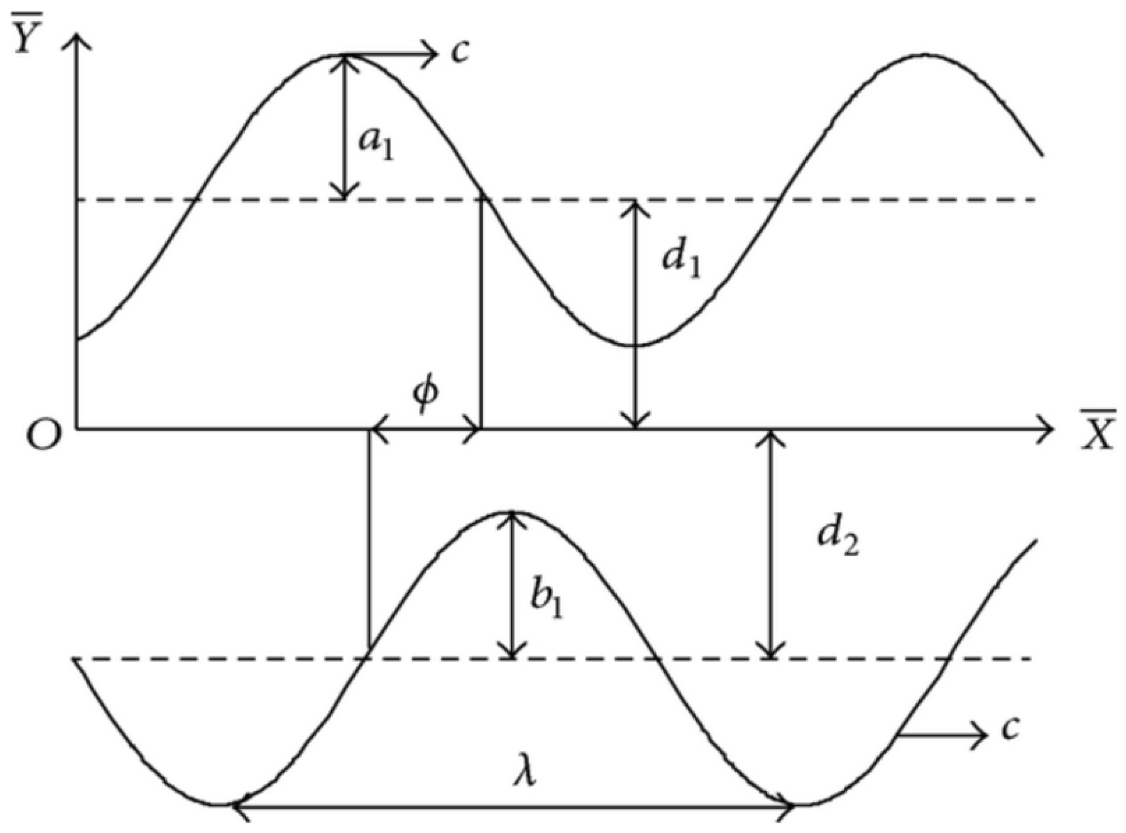
Abstract
:1. Introduction
2. Governing Equations
3. Entropy Generation Analysis
4. Series Solution
5. Discussion
6. Conclusions
- (i)
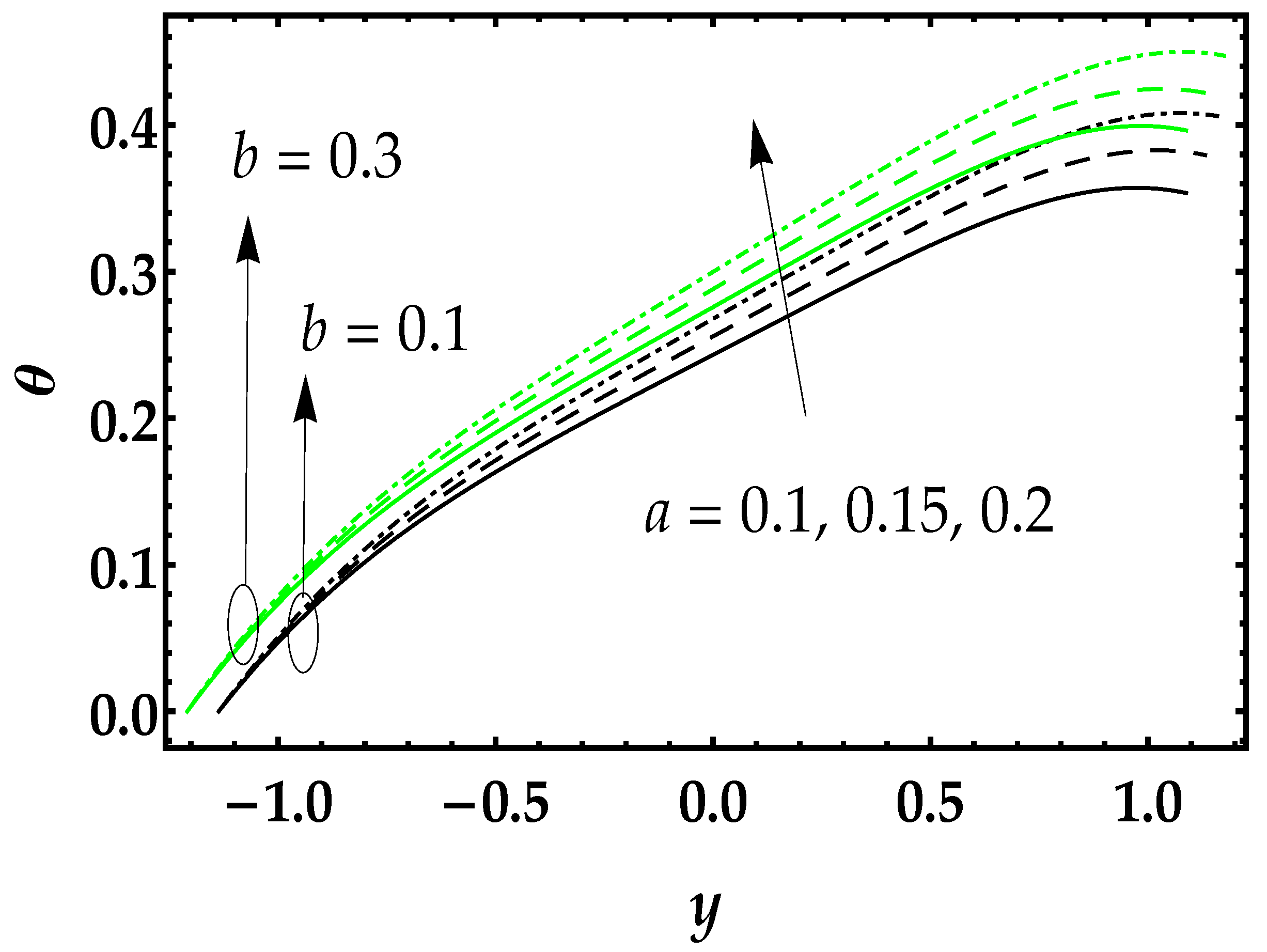
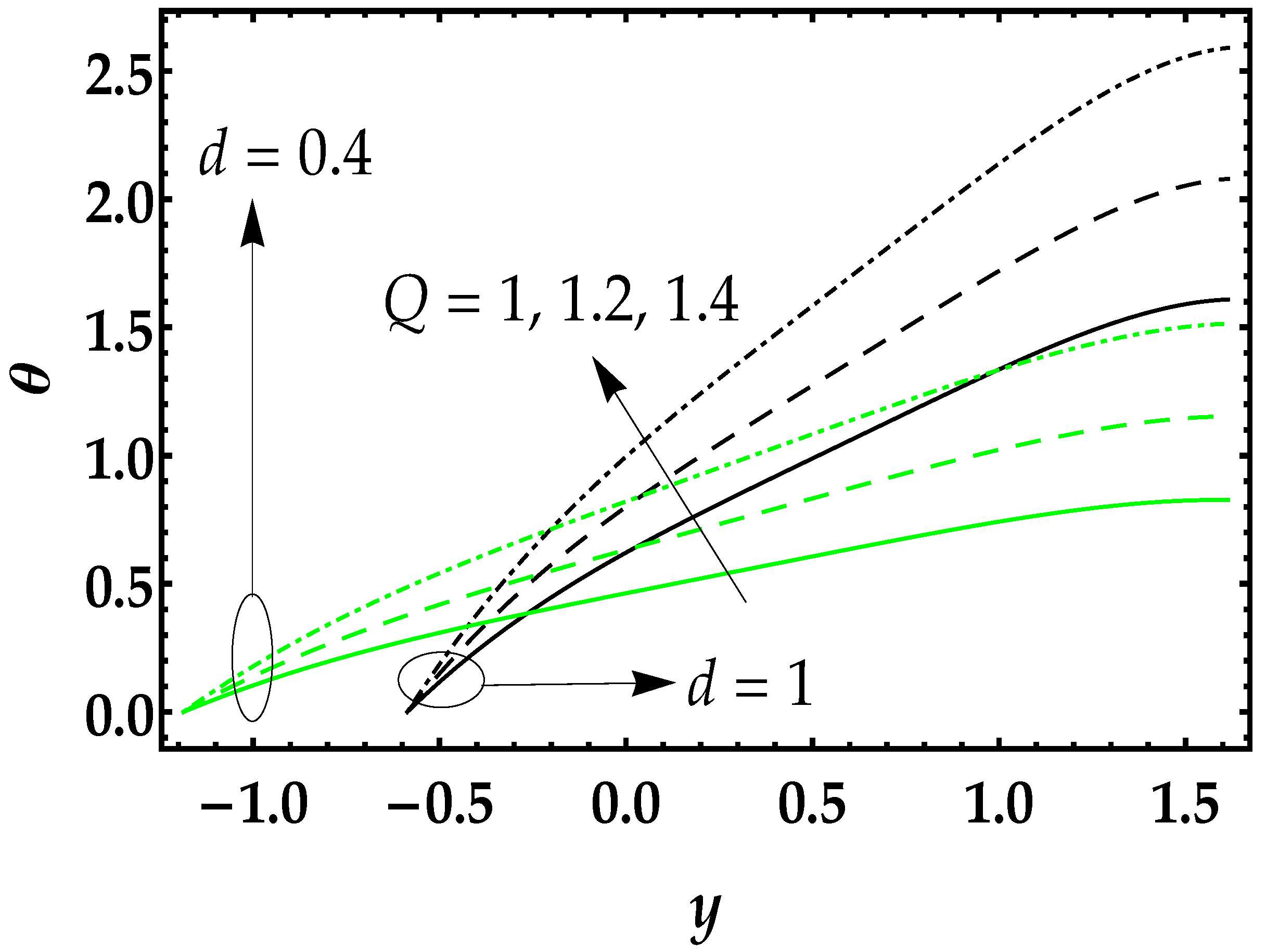
- It was noticed that the temperature profile revealed an increasing behavior by increasing the amplitude in the upper and lower region;
- (ii)
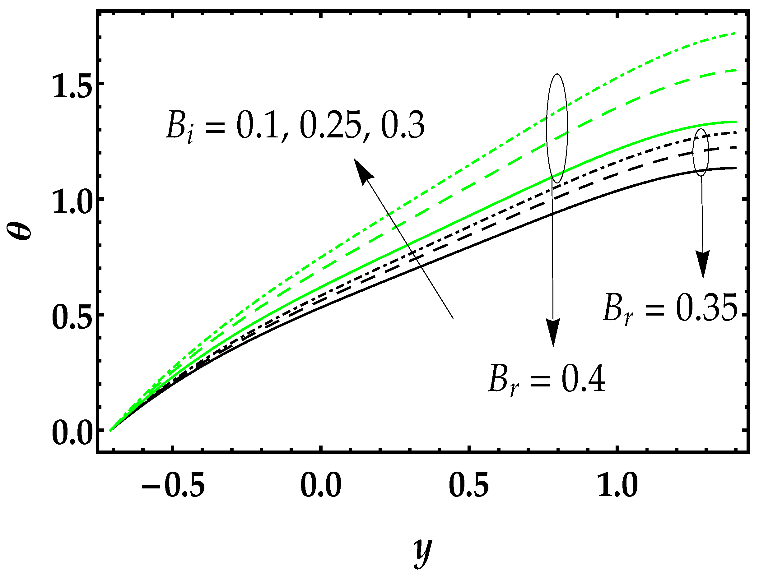
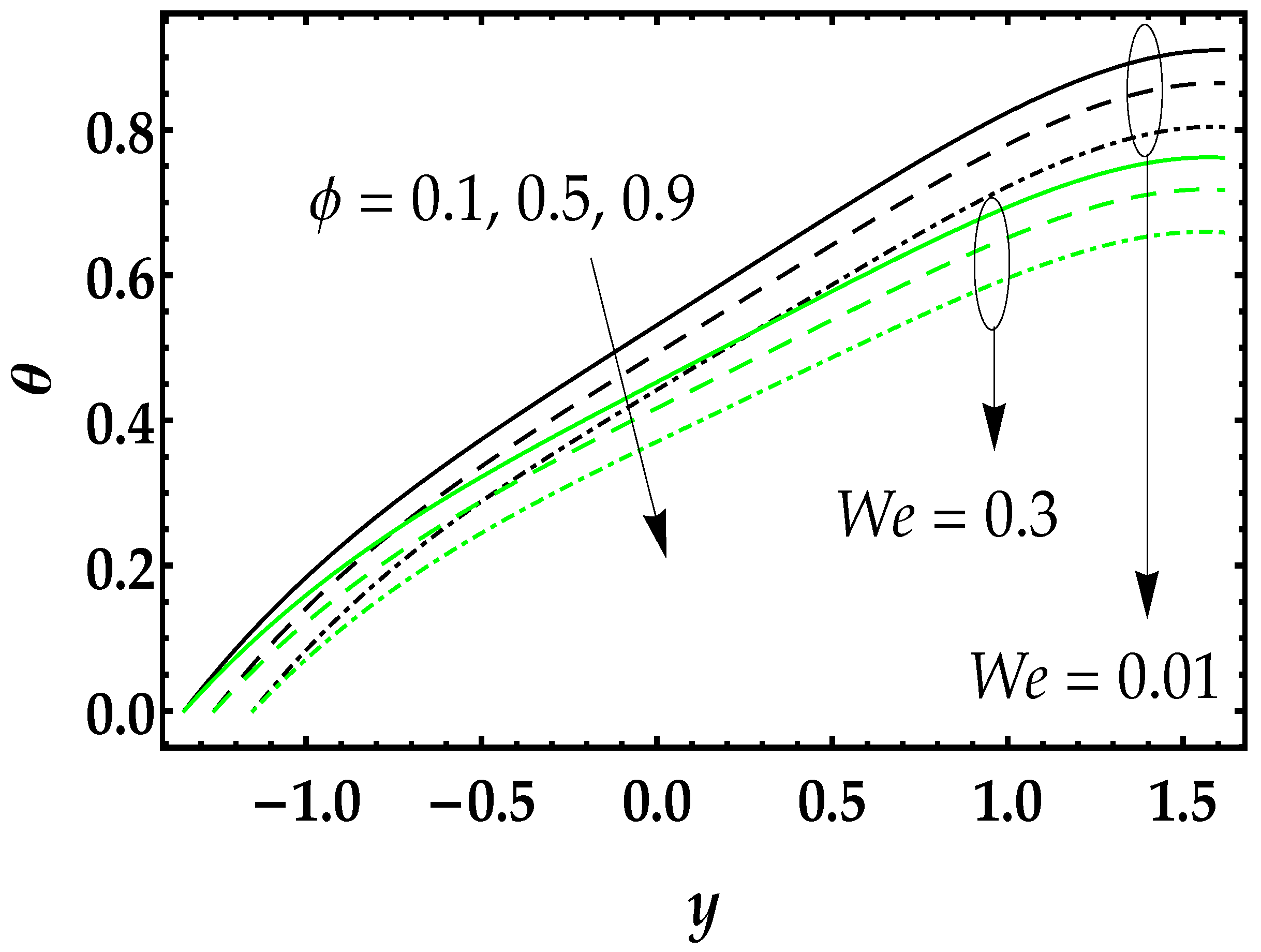
- The Biot number and Brinkman number significantly enhanced the temperature profile, whereas the behavior is converse for the phase difference parameter and Weissenberg number;
- (iii)
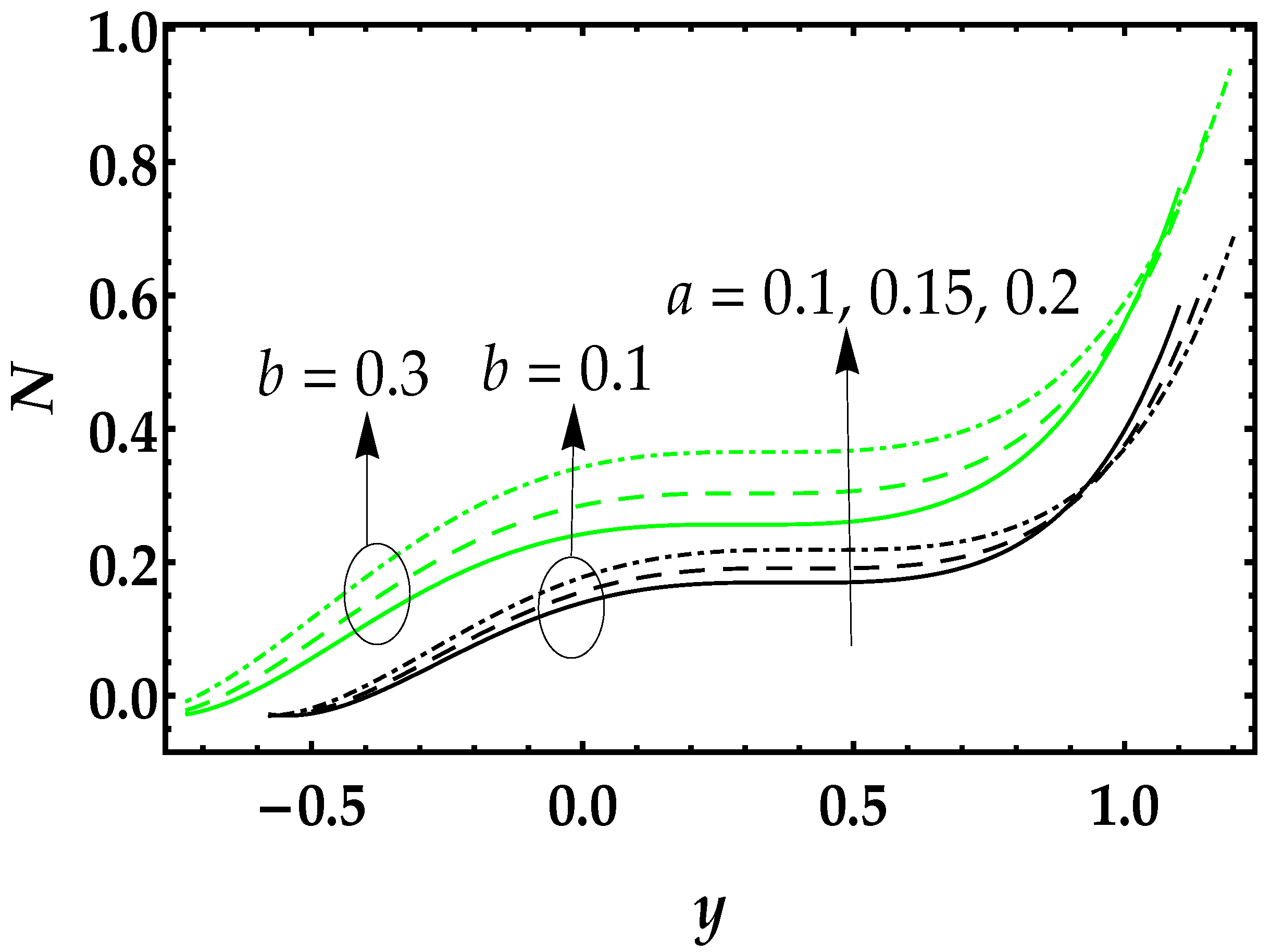
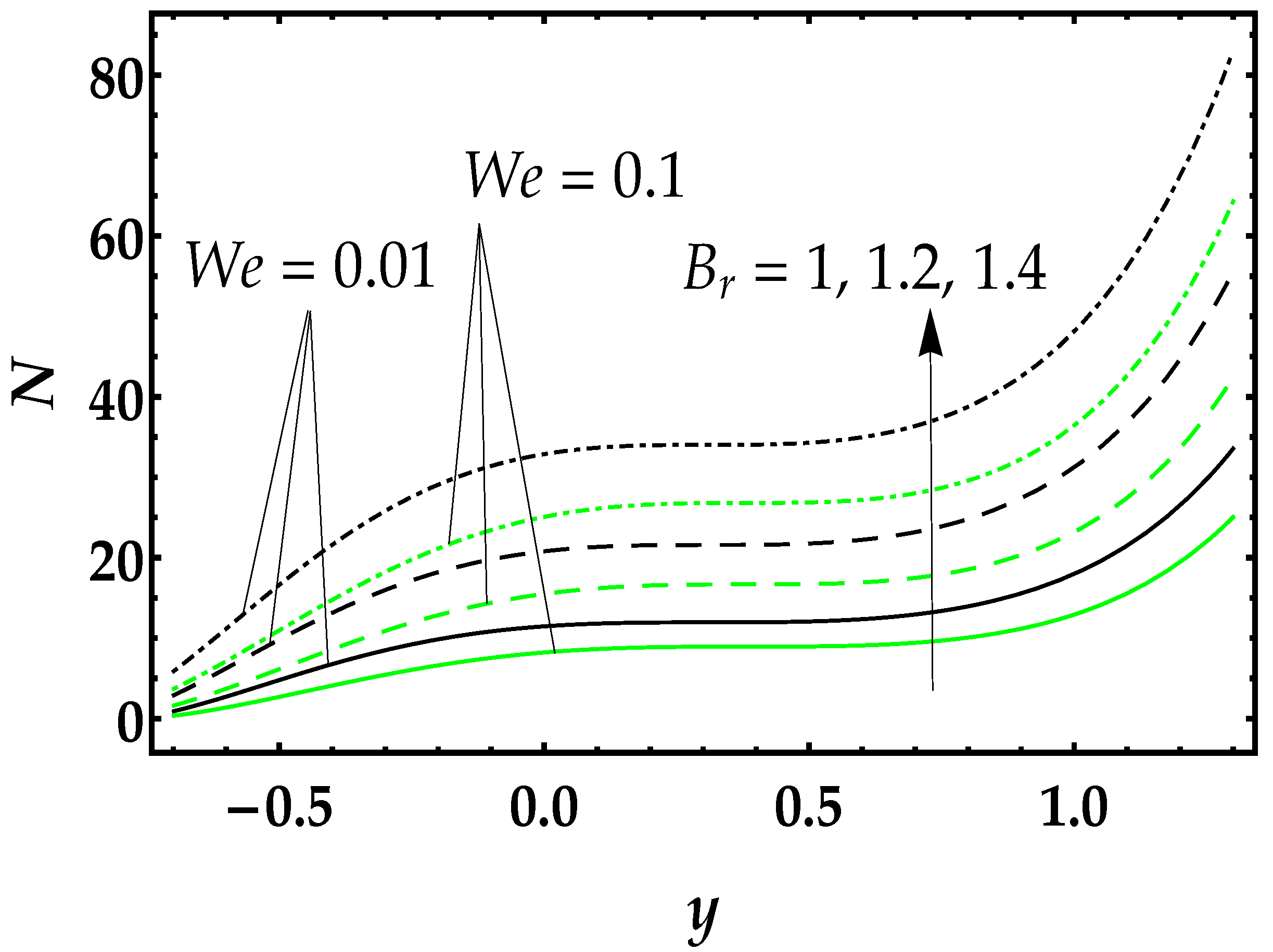
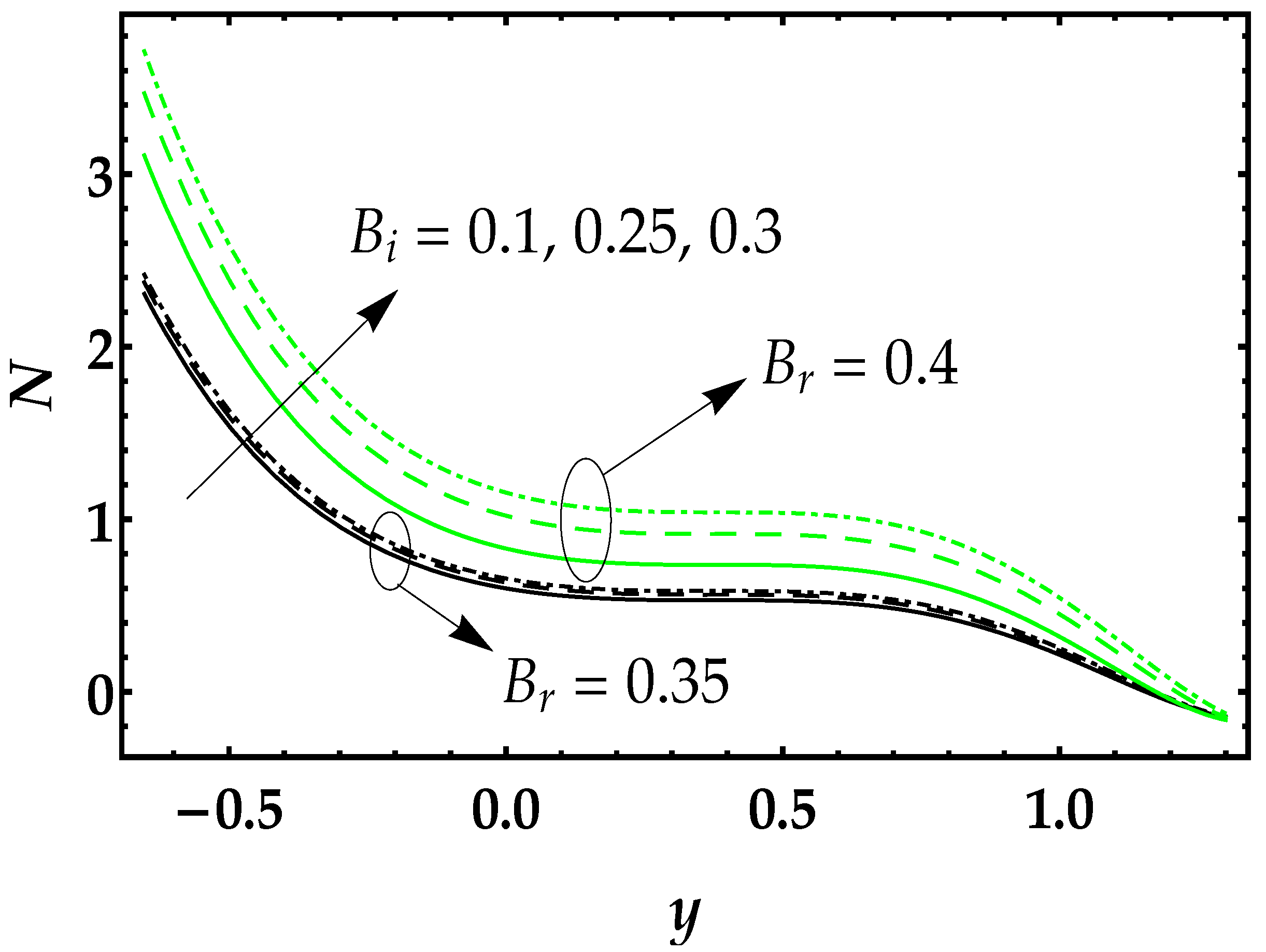
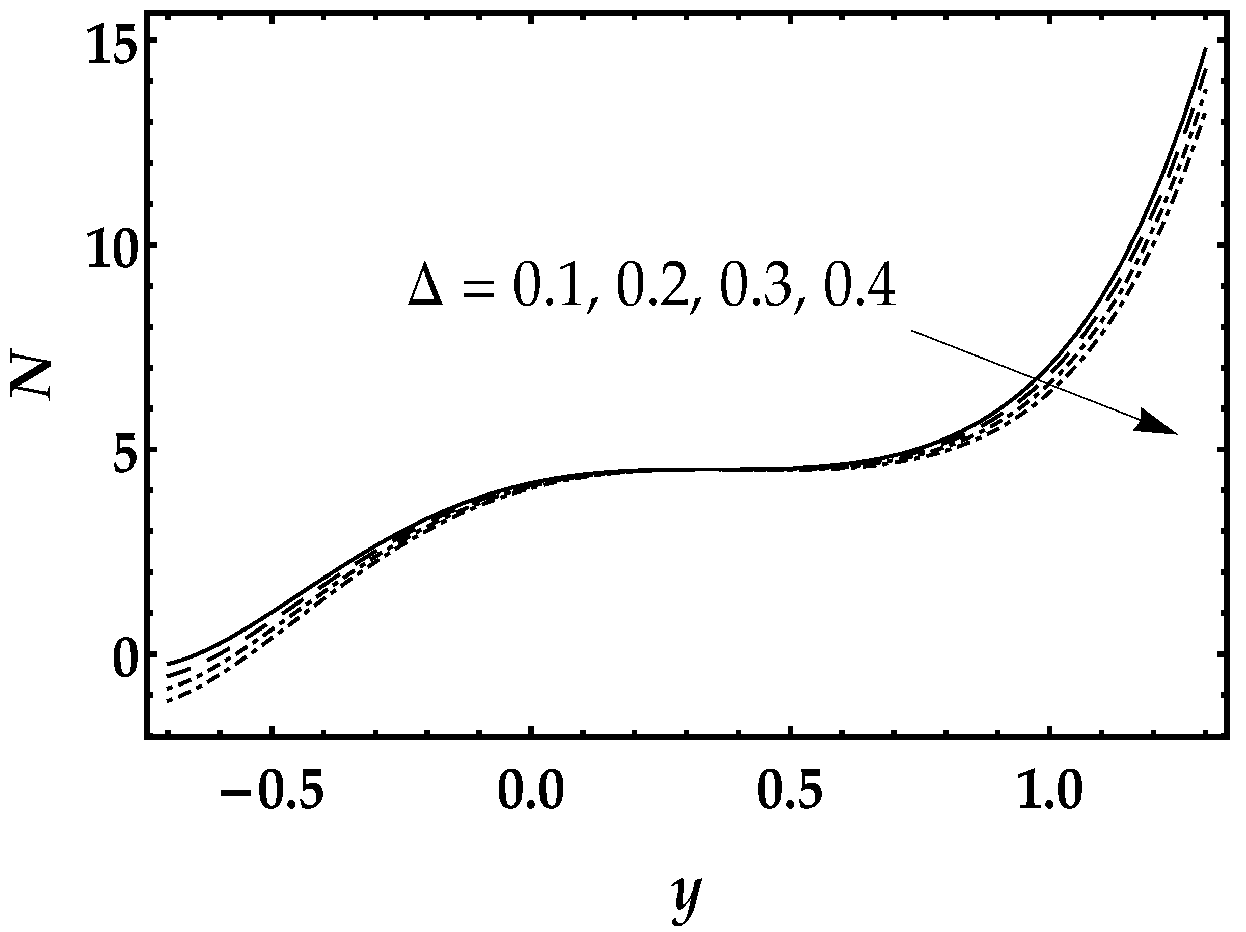
- Entropy profile represented an increment profile for higher values of Brinkmann number and Biot number, and a decrement behavior for the Weissenberg number;
- (iv)
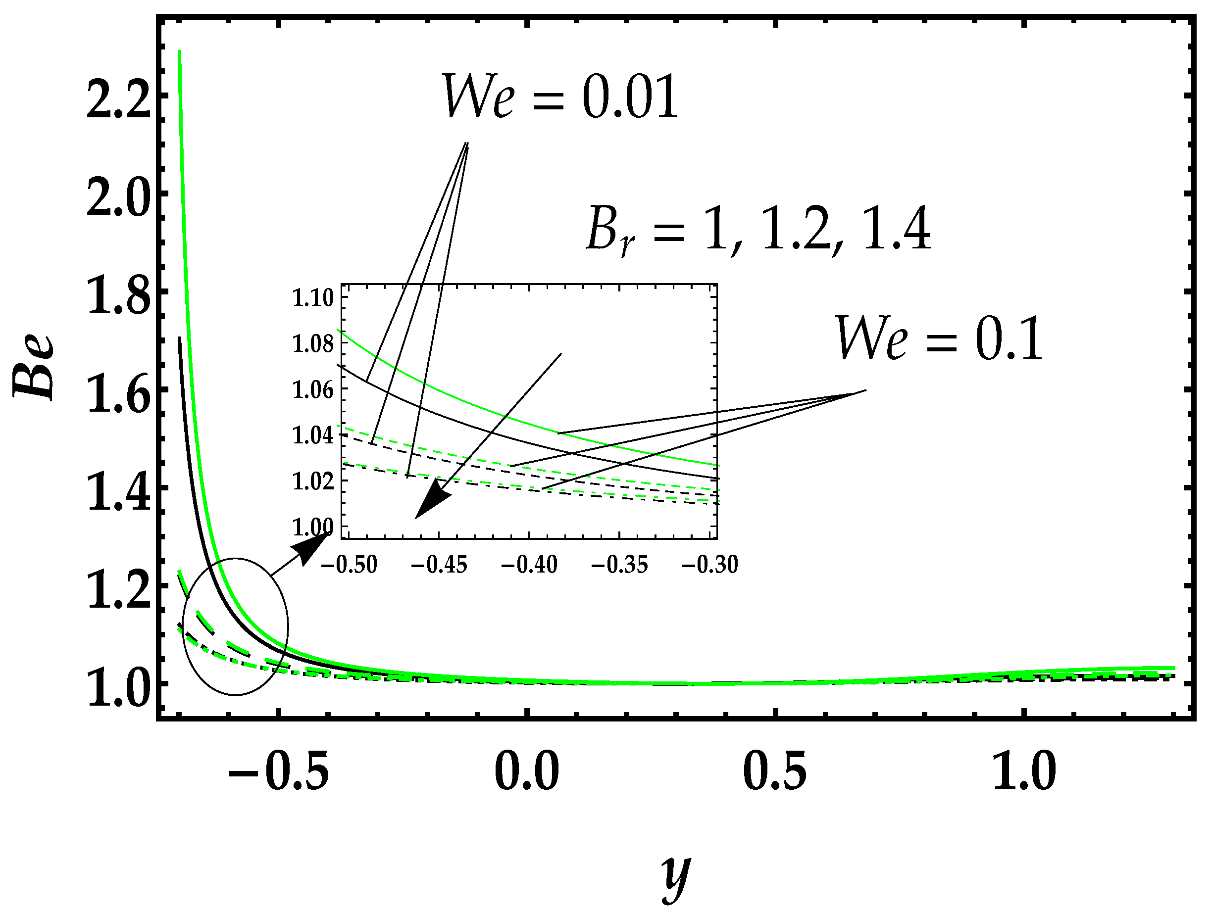
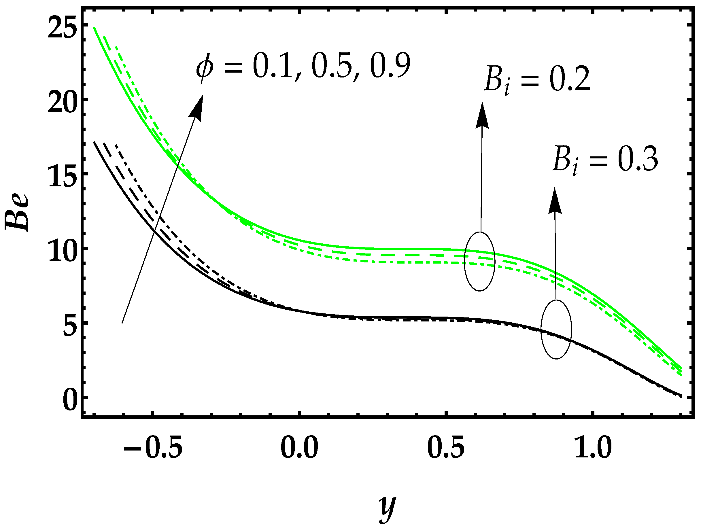
- The Weissenberg number boosedt the Bejan number profile, whereas it decreased due to the Biot number and Brinkman number;
- (v)
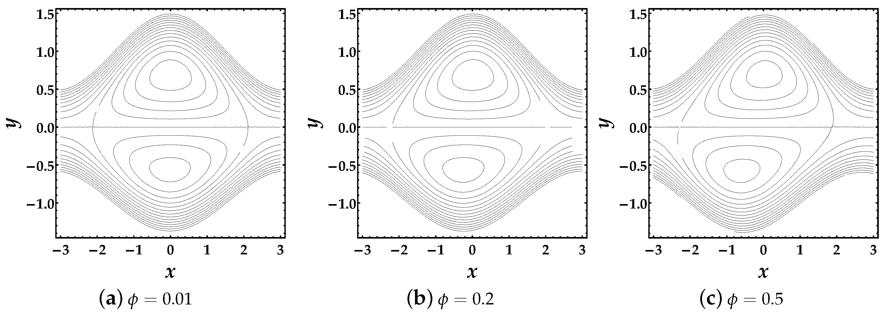
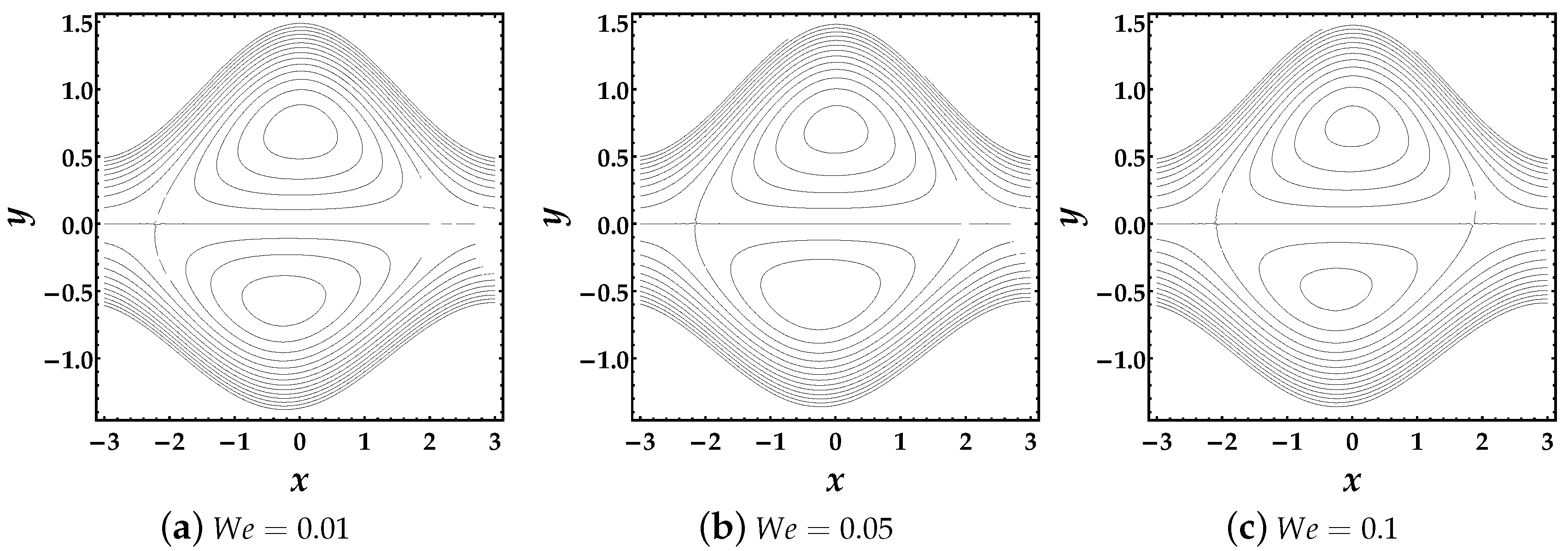
- Trapping mechanism showed that the phase difference parameter affected the magnitude of the trapped bolus, while the Weissenberg number not only affected the magnitude of the trapped bolus and the number of trapped boluses reduced in the lower region;
- (vi)
- The non-Newtonian results in the present study could be reduced to Newtonian fluid flow by taking
Author Contributions
Funding
Conflicts of Interest
Nomenclature
| channel width | |
| T | temperature |
| c | wave speed |
| time | |
| coordinate system | |
| velocity components | |
| stress tensor | |
| specific heat | |
| K | thermal conductivity |
| P | pressure |
| wave amplitude | |
| Reynold’s number | |
| Eckert number | |
| Prandtl number | |
| Brinkmann number | |
| Biot number | |
| Weissenberg number | |
| Bejan number | |
| entropy |
Greek Symbol
| phase difference | |
| density | |
| wavelength | |
| viscosity | |
| time constant | |
| wave number |
References
- Goldstein, M.; Goldstein, I.F. The Refrigerator and the Universe: Understanding the Laws of Energy; Harvard University Press: Cambridge, MA, USA, 1995. [Google Scholar]
- Kleiber, M. The Fire of Life: An Introduction to Animal Energetics; Robert E Kreiger Co.: New York, NY, USA, 1975. [Google Scholar]
- Holmes, F.L. Lavoisier and the Chemistry of Life: An Exploration of Scientific Creativity; Number 4; Univ. of Wisconsin Press: Madison, WI, USA, 1985. [Google Scholar]
- Silva, C.; Annamalai, K. Entropy generation and human aging: Lifespan entropy and effect of physical activity level. Entropy 2008, 10, 100–123. [Google Scholar] [CrossRef] [Green Version]
- Van Dinh, Q.; Vo, T.Q.; Kim, B. Viscous heating and temperature profiles of liquid water flows in copper nanochannel. J. Mech. Sci. Technol. 2019, 33, 3257–3263. [Google Scholar] [CrossRef]
- Ghorbanian, J.; Celebi, A.T.; Beskok, A. A phenomenological continuum model for force-driven nano-channel liquid flows. J. Chem. Phys. 2016, 145, 184109. [Google Scholar] [CrossRef]
- Silva, C.A.; Annamalai, K. Entropy generation and human aging: Lifespan entropy and effect of diet composition and caloric restriction diets. J. Thermodyn. 2009, 2009, 186723. [Google Scholar] [CrossRef] [Green Version]
- Hershey, D. Lifespan and Factors Affecting It: Aging Theories in Gerontology; Charles C. Thomas Publisher: Springfield, MA, USA, 1974. [Google Scholar]
- Hershey, D.; Wang, H.H. A New Age-Scale for Humans; Lexington Books: Lexington, KY, USA; Toronto, ON, Canada, 1980. [Google Scholar]
- Rahman, M.A. A novel method for estimating the entropy generation rate in a human body. Therm. Sci. 2007, 11, 75–92. [Google Scholar] [CrossRef]
- Aoki, I. Entropy flow and entropy production in the human body in basal conditions. J. Theor. Biol. 1989, 141, 11–21. [Google Scholar] [CrossRef]
- Annamalai, K.; Puri, I.K.; Jog, M.A. Advanced Thermodynamics Engineering; CRC Press: Boca Raton, FL, USA, 2011. [Google Scholar]
- Bejan, A. Constructal theory: From thermodynamic and geometric optimization to predicting shape in nature. Energy Convers. Manag. 1998, 39, 1705–1718. [Google Scholar] [CrossRef]
- Bejan, A. The tree of convective heat streams: Its thermal insulation function and the predicted 3/4-power relation between body heat loss and body size. Int. J. Heat Mass Transf. 2001, 44, 699–704. [Google Scholar] [CrossRef]
- Rashidi, M.; Kavyani, N.; Abelman, S. Investigation of entropy generation in MHD and slip flow over a rotating porous disk with variable properties. Int. J. Heat Mass Transf. 2014, 70, 892–917. [Google Scholar] [CrossRef]
- Komurgoz, G.; Arikoglu, A.; Ozkol, I. Analysis of the magnetic effect on entropy generation in an inclined channel partially filled with a porous medium. Numer. Heat Transf. Part A Appl. 2012, 61, 786–799. [Google Scholar] [CrossRef]
- Rashidi, M.; Keimanesh, M.; Bég, O.A.; Hung, T. Magnetohydrodynamic biorheological transport phenomena in a porous medium: A simulation of magnetic blood flow control and filtration. Int. J. Numer. Methods Biomed. Eng. 2011, 27, 805–821. [Google Scholar] [CrossRef]
- Akbar, N.S.; Raza, M.; Ellahi, R. Peristaltic flow with thermal conductivity of H2O+ Cu nanofluid and entropy generation. Results Phys. 2015, 5, 115–124. [Google Scholar] [CrossRef] [Green Version]
- Rashidi, M.; Bhatti, M.; Abbas, M.; Ali, M. Entropy generation on MHD blood flow of nanofluid due to peristaltic waves. Entropy 2016, 18, 117. [Google Scholar] [CrossRef] [Green Version]
- Akbar, N.; Raza, M.; Ellahi, R. Endoscopic Effects with Entropy Generation Analysis in Peristalsis for the Thermal Conductivity of 2 HO Nanofluid. J. Appl. Fluid Mech. 2016, 9, 1721–1730. [Google Scholar]
- Abbas, M.; Bai, Y.; Rashidi, M.; Bhatti, M. Analysis of entropy generation in the flow of peristaltic nanofluids in channels with compliant walls. Entropy 2016, 18, 90. [Google Scholar] [CrossRef]
- Bhatti, M.M.; Abbas, M.A.; Rashidi, M.M. Entropy Generation for Peristaltic Blood Flow with Casson Model and Consideration of Magnetohydrodynamics Effects. Walailak J. Sci. Technol. (WJST) 2017, 14, 451–461. [Google Scholar]
- Ranjit, N.; Shit, G. Entropy generation on electro-osmotic flow pumping by a uniform peristaltic wave under magnetic environment. Energy 2017, 128, 649–660. [Google Scholar] [CrossRef]
- Majee, S.; Shit, G. Numerical investigation of MHD flow of blood and heat transfer in a stenosed arterial segment. J. Magn. Magn. Mater. 2017, 424, 137–147. [Google Scholar] [CrossRef]
- Bhatti, M.; Sheikholeslami, M.; Zeeshan, A. Entropy analysis on electro-kinetically modulated peristaltic propulsion of magnetized nanofluid flow through a microchannel. Entropy 2017, 19, 481. [Google Scholar] [CrossRef]
- Ellahi, R.; Zeeshan, A.; Hussain, F.; Asadollahi, A. Peristaltic blood flow of couple stress fluid suspended with nanoparticles under the influence of chemical reaction and activation energy. Symmetry 2019, 11, 276. [Google Scholar] [CrossRef] [Green Version]
- Prakash, J.; Tripathi, D.; Tiwari, A.K.; Sait, S.M.; Ellahi, R. Peristaltic Pumping of Nanofluids through a Tapered Channel in a Porous Environment: Applications in Blood Flow. Symmetry 2019, 11, 868. [Google Scholar] [CrossRef] [Green Version]
- Mekheimer, K.S.; Zaher, A.; Abdellateef, A. Entropy hemodynamics particle-fluid suspension model through eccentric catheterization for time-variant stenotic arterial wall: Catheter injection. Int. J. Geom. Methods Mod. Phys. 2019, 16, 1950164. [Google Scholar] [CrossRef]


© 2020 by the authors. Licensee MDPI, Basel, Switzerland. This article is an open access article distributed under the terms and conditions of the Creative Commons Attribution (CC BY) license (http://creativecommons.org/licenses/by/4.0/).
Share and Cite
Riaz, A.; Bhatti, M.M.; Ellahi, R.; Zeeshan, A.; M. Sait, S. Mathematical Analysis on an Asymmetrical Wavy Motion of Blood under the Influence Entropy Generation with Convective Boundary Conditions. Symmetry 2020, 12, 102. https://doi.org/10.3390/sym12010102
Riaz A, Bhatti MM, Ellahi R, Zeeshan A, M. Sait S. Mathematical Analysis on an Asymmetrical Wavy Motion of Blood under the Influence Entropy Generation with Convective Boundary Conditions. Symmetry. 2020; 12(1):102. https://doi.org/10.3390/sym12010102
Chicago/Turabian StyleRiaz, Arshad, Muhammad Mubashir Bhatti, Rahmat Ellahi, Ahmed Zeeshan, and Sadiq M. Sait. 2020. "Mathematical Analysis on an Asymmetrical Wavy Motion of Blood under the Influence Entropy Generation with Convective Boundary Conditions" Symmetry 12, no. 1: 102. https://doi.org/10.3390/sym12010102