The Systematic Optimization of Train Formation in Loading Stations

Abstract

This paper presents the formulation of a train formation problem in rail loading stations (TFLS) from the systematic perspective. Several patterns of train formation are analyzed thoroughly before modeling, including direct single-commodity trains, direct multi-commodity trains created in the loading stations, and direct trains originating from reclassification yards. One of the crucial preconditions is that the loading and unloading efficiencies in the loading stations and the relational unloading stations are symmetric. Based on this, a non-linear 0–1 programming model is designed with the aim of minimizing the total car-hour cost incurred by the loading, unloading, and reclassification operations, and the commercial software Lingo is employed as the solving approach. A small-scale example is carried out first to illustrate the validity of the presented model and the effectiveness of the proposed method. Then, a series of numerical cases are devised to test the model and solving approach. The computational results show that our model can be regarded as a theoretical foundation of the TFLS problem.

1. Introduction

The transportation of bulk materials occupies an importation position in rail operation. The European Commission declared in documents their aim to shift road freights to other modes such as rail or waterborne transport [1]. Governments of European countries also proposed relative documents targeted at reducing the freight volume of road transportation. Countries in Asia also recognized the severity of the unbalanced transportation structure. China made the goal of transporting bulk commodities in major coastal ports by rail or waterborne transport [2]. The present state provides a precious opportunity for railroads to develop direct single-commodity train transportation.

The train formation plan in loading stations (TFLS) is one of the crucial foundations of rail operation (Martinelli and Teng [3]; Lin et al. [4]), which can provide a bulk train service (block) for bulk materials in loading stations. Unlike train services between reclassification yard pairs, the bulk train services are defined to originate from certain loading stations and destinate at corresponding unloading stations. According to TFLS, three of the most practical and crucial train formation patterns are elaborated and analyzed, including direct single-commodity trains, multi-commodity trains, and direct trains.

The optimization of TFLS problem aims at determining the optimal train services among loading and unloading stations for bulk materials, with the aim of minimizing the total car-hour consumption induced by the loading, unloading, and reclassification operations and satisfying practical conditions and logical constrains among decision variables.

This paper is organized as follows: in Section 2 a brief review of existing literature dedicated to train formation in both yards and loading stations is provided. The advantages of modeling techniques of TFP can be regarded as references to the TFLS problem. Section 3 discusses the train formation problem in loading stations through an artificial line rail network. Section 4 formulates the mathematical model for TFLS and explores its peculiarities. A small-scale case is employed to verify the validity of the model in Section 5, and a sensitivity analysis is then carried out to test the efficiency of the solving approach. Finally, Section 6 concludes the present work and delineates the further directions.

2. Literature Review

The train formation plan (TFP), as a general rule, is referred to as the critical document which can determine between which yard pairs should train services be provided in a rail network and the shipping routes of individual railcars. The problem we focus on in this work is optimized based on the TFP problem. Consequently, the concepts, modeling techniques, and the solving approaches of the TFP problem can be taken as references for the train formation problem in loading stations (TFLS).

Typical and excellent modeling methodologies of TFP should be noted. Bodin et al. [5] proposed the initial programming model for the railroad blocking problem, with the aim of determining the simultaneously optimized classification strategy for all yards in a rail system. Although the model is non-linear, the constraints it involves, for example, the balance equations, capacity constraints, and pure strategy constraints, can be regarded as an inspiration to the following studies: Assad [6] presented a cost-oriented dynamic programming model based on a line network in the consideration of flow balance and motive power constraint and other simple but explicit constraints. Haghani [7] developed a mixed-integer programming model with non-linear objective function and linear constraints, which was not only involved with the train routing and make-up, but also concerned with the empty car distribution problem. Since the models of TFP are usually complex, researchers made great efforts to release variables and develop ingenious heuristic procedures. Crainic et al. [8] devised an efficient heuristic algorithm based on decomposition and column generation techniques. They tested their programming model and solving approach through a real-world case of Canadian National Railroads, including 107 nodes, 95 links, and around 7000 traffic classes. Ahuja et al. [9] developed a very large-scale neighborhood (VLSN) search which can solve the problem to near optimality. Lin et al. [10] presented an efficient simulated annealing algorithm and obtained a remarkable solution of a large-scale problem including 5544 stations and more than 520,000 shipments in China’s railway system. For an overall and comprehensive review of TFP studies in the literature, the readers can refer to Cordeau et al. [11] and Haghani [12]; for a survey of the application of rail service design, the readers can refer to Gorman et al. [13].

Yaghini et al. [14] analyzed the costs associated with the train formation process, including the fixed cost for operating trains and variable cost for refueling, as well as locomotive and classification yard facilities. With the aim of minimizing the total costs, a linear programming model was devised with integer variables indicating the frequencies of trains and continuous variables representing the amounts of flows, while observing the limits on the train capacities, yard capacities, the number of trains (blocks) that can be formed in a yard, and flow conservation. A simulated annealing algorithm was proposed for the train formation model, and 25 test problems were generated to evaluate the performance of the proposed solving method and CPLEX software. The computational results could verify the efficiency and effectiveness of the proposed algorithm. Their study was profound and inspiring, whereas there existed some demerits in the presented mathematical model; moreover, their model could not be applied to the train formation problem in loading stations (TFLS). Our contribution with respect to the mathematical model over Yaghini et al. [14] is as follows:

(i) The costs incurred by forming trains in yards are roughly classed into two types, the fixed and variable costs. In the variable cost, the shunting cost is included, which is corresponds to the number of stops for a train in the intermediate stations. It indicates that the stopping (reclassification) strategy for each train was already determined; however, it should be optimized since the shunting cost is related to the stopping plan (Lin et al. [10]). More importantly, not all the demands are taken by the corresponding outbound trains at the same time. Usually, they arrive in an uneven pattern, which adds difficulties in formulating the accumulation process (the formulation of the accumulation process can be found at the 2019 railroad problem solving competition (https://connect.informs.org/railway-applications/new-item3/problem-solving-competition681)). Different from the work of Yaghini et al. [14], the TFLS is exclusive of the accumulation process of demands, since the railcars are stored in special lines of the loading stations. Furthermore, the costs generated in the loading and unloading stations are different from these generated in the yards, which are influenced by the loading and unloading efficiencies, train sizes, the volumes of commodities, and the pattern of train formations.

(ii) The design of the variables in Yaghini et al. [14] is actually not in accordance with practical application. A continuous variable is employed to represent the amount of flow of a certain demand on a train, which implies that one demand can be separated into several railcar flows. In fact, the split of one single demand is not allowed in railway operation. A freight demand, owned by a shipper, should be wholly and indivisibly transported by one or several trains. Whereas, in the research of Yaghini et al. [14], the operation of trains is fixed, i.e., the train to be formed is pre-determined. Actually, only the problem of which demand should be taken by which train is studied. On the other hand, in our research, three categories of train formations are firstly discussed and the corresponding decision variables are designed; then, a mathematical model is formulated aimed at solving (a) which train should be operated in the loading stations, (b) which demands should be combined together, and (c) which demand should be collected by which train. Additionally, and importantly, the bulk demands are absolutely not allowed to be separated in our model, and a relational constraint is proposed to ensure that the demands originating from the loading stations can be delivered to the corresponding unloading stations.

Chen et al. [15] investigated the one-block train formation problem, and a linear programming model was established aimed at minimizing the total accumulation cost and reclassification delay, limited by the reclassification capacity and the number of sorting tracks. A linear and clear equation for counting the number of cars contained in blocks was proposed, which can be regarded as an excellent reference for formulating the traffic flows of shipments in the rail network. However, as mentioned before, the TFLS is different from TFP because the former occurs in the loading station, while the latter happens in reclassification yards. There exist discrepancies between loading stations and reclassification yards; for example, loading stations do not have the capability to reclassify railcars; therefore, there are no such reclassification capacity and sorting track constraints in TFLS. The optimization results of TFP are actually the preliminary works of TFLS, which also prevents the mathematical model of TFP from being employed in the TFLS problem. Due to the abovementioned reasons, the linear mathematical model proposed by Chen et al. [15] cannot serve for the train formation problem arising from loading stations.

Xiao et al. [16] focused on the block-to-train assignment problem and proposed an integer programming model considering service design cost savings, the train operation cost savings, the car-hour consumption savings in the accumulation process, and in the attachment and detachment operations, and the waiting car-hour consumption savings. A heuristic approach based on the genetic algorithm and a tabu search was then developed to solve the large-scale problems. A multi-block train service network is considered in their research instead of a single-block train service.

As one of the foundations of operation in railway, the optimization of the train formation plan between yards can be found in numerous studies, whereas the works related to the train formation in loading stations are actually extremely scarce. The long negligence of railway bulk transportation might be the reason for the inadequate studies on TFLS. Lin et al. [17] formulated a non-linear 0–1 programming model based on the car-hour consumption in loading areas, itineraries, and unloading areas. However, the car-hour costs per car incurred by the loading, unloading, and reclassification operations were set as constant, which is not specific enough. Moreover, the solving approach of this model was to enumerate all the variables and constraints, which is not suitable for large-scale cases. Motivated by this study, Cao et al. [18] analyzed the inventory costs in loading and unloading stations, but no improvement on the solving approach was proposed. The validity of the non-linear programming model was verified by the enumeration method. Fan et al. [19] classed the trains originating from loading stations and specified the conditions to form these trains. From the perspective of logistics systems, Ji et al. [20] balanced the costs of railroads, shippers, and receivers under the constraints of loading and unloading capacities and flow exclusive conditions. However, the solving of the real-world case carried out in this work was the same as that by Lin et al. [17], which cannot be employed for large-scale cases either. Masek et al. [21] presented time-continuous and time-discrete models for transporting single-wagon consignments on railway networks. One alternative way of shipping wagons from loading stations to unloading stations was described in detail. However, the solving approach of the models and numerical examples were missing in this work. Zhao and Lin [22] proposed a linearized programming model based on the collection delay in loading stations, whereas the costs in unloading stations and intermediate reclassification yards were not taken into consideration, and the pattern of train formations was not universal.

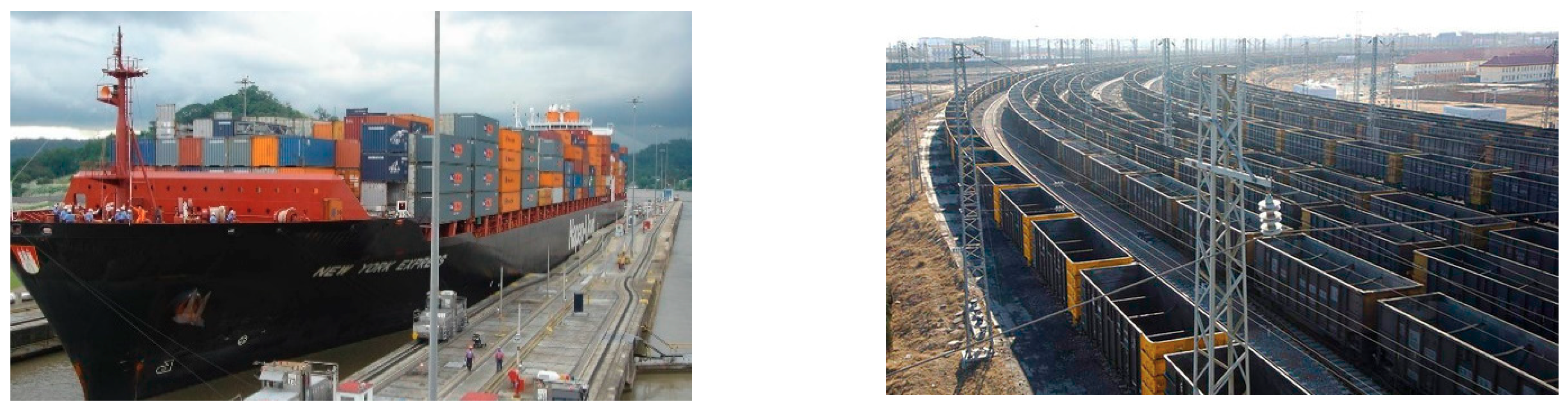
For other transportation modes, for example, maritime navigation, in the work of Iris et al. [23], the flexible ship loading problem (FSLP) was optimized, including the management of loading operations, and the planning and scheduling of transport vehicles. There are indeed certain similarities between the loading problems for seaport container terminals and for railway stations. For example, which specific container to load for each slot has the peculiarity of flexibility, and a corresponding variable is devised to optimize the best position for containers in the modeling process. In railway loading stations, it also needs to be determined which railcar flow should be arranged on which train, and a relational variable is also designed in our presented work. However, there actually exist differences between FSLP and TFLS; for example, operation time is included in the optimization target of FSLP but not in FTLS because delivery time is not a crucial element in railway bulk freight transport. Furthermore, the constraints considered in FSLP are much more diverse from those in TFLS since the loading vehicles of maritime navigation and railway transportation are containers and wagons (see Figure 1), respectively.

For most TFLS models constructed on the basis of constant costs incurred by loading, reclassification, and unloading operations, the elaborated classification of costs is absent, and the train formation patterns are not comprehensive. Moreover, the solving approaches proposed are not appropriate for large-scale cases. This actually stimulated us to develop modeling methodologies, accompanied by exhaustive classified car-hour costs induced in the loading and unloading stations and reclassification yards. The contributions of this present work are given below.

The train formations in loading stations are classed on the basis of the origins of trains and the number of bulk material categories: direct single-commodity trains, direct multi-commodity trains, and direct trains, which can be regarded as a fundamental aid allowing us to construct the mathematical model. The car-hour costs incurred by the loading, reclassification, and unloading operations are then specifically formulated in accordance with the category of train formation. A non-linear 0–1 integer programming model is established, and an artificial case is carried out to verify the validity of the model.

3. Problem Description

The shipping strategies of bulk commodities are as imperative as those of general shipments transported between yards. An appropriate shipping strategy should satisfy the following conditions: for each shipment, (i) it can be delivered to the corresponding destination; (ii) it cannot be split into several flows either in the loading station or be disassembled into different railcars in the reclassification yards. The optimization of train formation in loading stations aims at determining the systematically optimal shipping strategy of bulk commodities, including the decisions of which direct bulk services should be provided between the loading area and the unloading area, which small-volume bulk flows should be added to which direct train, and which bulk flows should be combined together.

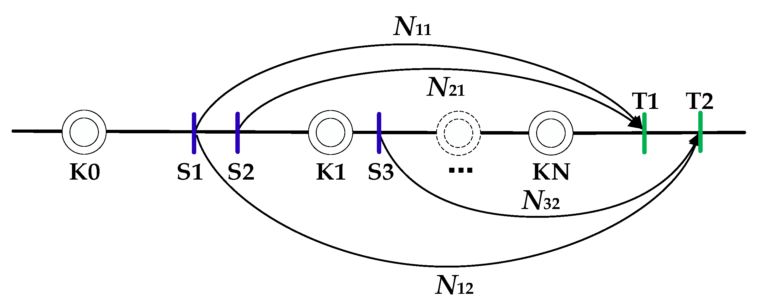
For a better understanding of shipping strategies of bulk materials and train formations in loading stations, a small-scale artificial case is presented in Figure 2.

There are three loading stations (S1, S2, and S3, blue vertical lines), two unloading stations (T1 and T2, green vertical lines), and several reclassification yards (K0, K1,…, KN, concentric circles) in the line network in Figure 2. Four bulk shipments (black horizontal lines with arrows at the end) are included in the network, which are steel wagon flow $N_{11}$ from S1 to T1 with the volume of 23 cars per day, steel flow $N_{12}$ from S1 to T2 with 40 cars per day, coal flow $N_{21}$ from S2 to T1 with 236 cars per day, and mineral flow $N_{32}$ from S3 to T2 with 14 cars per day. As an illustrative example, it is assumed that, between each loading station and unloading station, a bulk train service can be provided. There are plenty of combinations for shipping all the wagon flows on the tentative bulk train service network (see Figure 3).

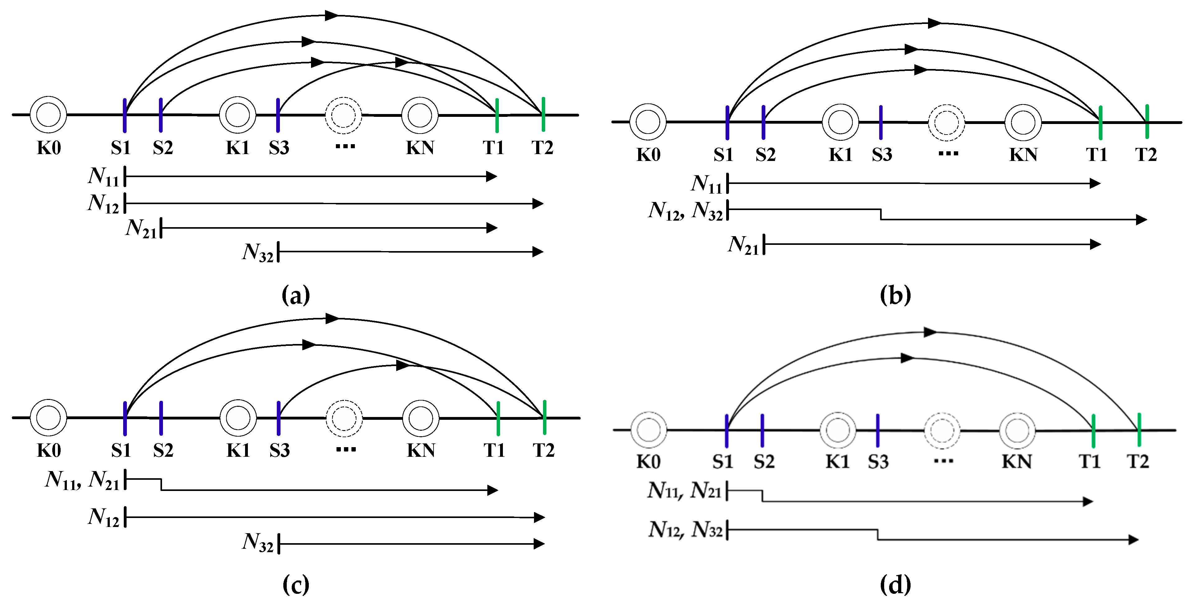
The black arrows in the middle represent the bulk train service in Figure 3. As shown in Figure 3a, four bulk train services are provided in the line network, and thereby four bulk shipments are transported separately and directly to the corresponding destinations, without any combinations in the loading stations or reclassifications in the itineraries. In this scenario, each train is loaded with one single commodity from one loading station, which is called a direct single-commodity train (DSC train). It is actually economical and rational to transport high-volume shipments via direct train services. For example, the traffic volume of the coal shipment $N_{21}$ is 236 cars per day, which is perfectly suitable for a DSC train. Actually, in China, if the volume of a shipment is more than 0.5 million tons per year, a DSC train can be provided for delivering this shipment. However, for other bulk shipments in Figure 3a, it is unpractical for them to be shipped by DSC trains.

The steel commodity in loading station S1 is combined with the mineral commodity in S3, as shown in Figure 3b, which is produced by the removed bulk train service from S3 to T2. Since shipment $N_{32}$ is unable to be shipped directly, it has to be combined with other wagon flows with the same unloading station, for example, shipment $N_{12}$. Here, in the loading area, the combination of wagon flows with different destinations is not considered in this work. Thereby, the bulk shipments can be combined together in the loading area only if they have the same unloading stations. We define the trains originating from the loading area, destinated directly to the unloading stations with multiple commodities, as direct multi-commodity trains (DMC trains). Moreover, the combinations of relatively small-volume bulk shipments can contribute to a more economical and less operation-intensive transportation mode in railway.

A similar combination of bulk shipments in the loading area can be found in Figure 3c. In this scenario, the bulk train service from S2 to T1 is removed from the line network, which leads to the combination of bulk shipments $N_{11}$ and $N_{21}$.

Figure 3d incorporates the scenarios shown in Figure 3b,c, in which only two bulk train services are needed: from S1 to T1 and from S1 to T2. It can be concluded that, as the combinations of flows increase, fewer bulk train services are required.

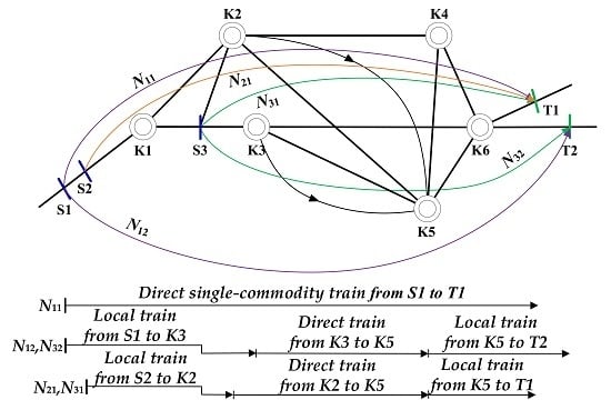
A diverse scenario is described in Figure 3e,f. Compared with the service network in Figure 3a, a train service from the reclassification yard K1 to KN is newly provided (other train services between omitted yards are not listed here and not taken as examples), and the bulk train services from S1 to T2 and from S2 to T1 are removed from the line network. Unlike organizing a train in the loading area, a direct train runs from K1 to KN. Since bulk shipments $N_{12}$ and $N_{21}$ cannot be delivered directly to the relational destinations, there are two alternative ways to carry out the transportation tasks. If both shipments $N_{12}$ and $N_{21}$ are placed on the direct train from K1 to KN, the local trains (including pick-up trains and sectional trains) will collect these shipments firstly from the loading area and then head for the reclassification yard K1, as shown in Figure 3e. There is another possibility that shipment $N_{21}$ is added to the DMC train created at loading station S1 (see Figure 3f). In this case, only shipment $N_{12}$ is placed on the direct train from K1 to KN.

Note that there is a train service (red dotted arc in Figure 3f) from the reclassification yard K0, which is a station at the rear of the loading area in this line network. The bulk shipments $N_{11}$, $N_{12}$, $N_{21}$, and $N_{32}$ can be added to this direct train originating from K0 only if a portion of loading capacity of this direct train is reserved for these bulk shipments. This scenario, however, is not considered in the systematic optimization of train formation in the loading area due to its high complexity.

The train formation in the loading stations was discussed thoroughly through the above line rail network. Based on the train service network, the direct single-commodity trains, direct multi-commodity trains, and direct trains were created in the loading stations and yards to ship bulk commodities in the loading area. The comprehensive programming model of TFLS is devised and elaborated on in Section 4.

4. Mathematical Model

A general mathematical model of the train formation problem in loading stations is formulated in this section. The prime focus of this model is to determine (i) which bulk shipments can be combined together in the loading area, (ii) between which pairs of yards or loading–unloading stations should train services be provided, and (iii) which train should be created in the loading stations and yards. The car-hour costs incurred by loading, unloading, and reclassification operations are analyzed in the model, while satisfying the flow exclusive constraint, carrying capacity constraint, and several logical constraints among decision variables. Note that the choices of the physical paths of shipments are not taken into consideration, which are pre-defined instead of incorporating them with optimization.

The sets, parameters, and variables are listed in

Table 1. The descriptions of notations.

Sets
$LS$	The set of all the loading stations in a rail network;
$US(s)$	The set of all the unloading stations corresponding to the loading station $s$ in a rail network;
$\phi \left(s^{\prime }\right)$	The set of all the possible loading stations for which DMC trains with the origin $s^{\prime }$ can serve;
$\rho \left(s,t\right)$	The set of all the potential satellite marshalling stations (first reclassification yard) for the bulk shipment from $s$ to $t$ if shipped via a direct train;
$\sigma \left(s,t\right)$	The set of all the destinations of the direct trains loaded with bulk commodities with origins $s$ and destinations $t$.
Parameters
$N_{st}^{}$	The amount of freight traffic of the bulk commodity from the loading station $s$ to the unloading station $t$, in cars per day;
$m_{st}^{}$	The size of a DSC train from the loading station $s$ to the unloading station $t$, in cars;
$m_{s^{\prime }{t}^{\prime }}^{}$	The size of a DMC train from the loading station $s^{\prime }$ to the unloading station $t^{\prime }$, in cars;
$m_{k\kappa }^{}$	The size of a direct train from the reclassification yard $k$ to yard $\kappa$, in cars;
${ℂ}_{st}^{}$	The average carrying capacity of each car of the DSC train originating from the loading station $s$ and destined to the unloading station $t$, in tons per car;
${ℂ}_{s^{\prime }{t}^{\prime }}^{}$	The average carrying capacity of each car of the DMC train from the loading station $s^{\prime }$ to the unloading station $t^{\prime }$, in tons per car;
${ℂ}_{k\kappa }$	The average carrying capacity of each car on the direct train from the reclassification yard $k$ to yard $\kappa$, in tons per car;
$e_s^{\mathrm{lo}}$	The average loading efficiency at the loading station $s$, in tons per hour;
$e_t^{\mathrm{un}}$	The average unloading efficiency at the unloading station $t$, in tons per hour;
$t_s^{\mathrm{local}}$	The average waiting time per car when the bulk shipments in the loading station $s$ are loaded onto the local trains and transported to the satellite reclassification yards, in hours;
$t_t^{\mathrm{local}}$	The average time consumption per car when the bulk shipments at the reclassification yard are waiting for the local trains in order to be delivered to the relational unloading station $t$, in hours;
$C^{\mathrm{block}}(k,\kappa )$	The available carrying capability of the train service from $k$ to $\kappa$, in cars per day;
${\tau }_k$	The unit operation delay at yard $k$ during the arriving, inspecting, classification, assembling, and departing processes, which are not influenced by the categories of commodities, in hours.
Decision variables
$x_{st}$	DSC train variable; it takes the value of one if commodity $\delta$ is shipped directly from the loading station $s$ to the unloading station $t$; otherwise, it is zero;
$x_{st}^{s^{\prime }{t}^{\prime }}$	DMC train variable; it takes the value of one if wagons from the same or different loading stations $s$ to the relational destinations $t$ are combined and transported together via the DMC train which originates from the loading station $s^{\prime }$ and is destined for the unloading station $t^{\prime }$; otherwise, it is zero;
$x_{st}^{k\kappa }$	Direct train variables; it takes the value of one if wagons from the loading station $s$ are taken via the sectional trains or pick-up trains and then shipped to the reclassification yard. After that, these wagons are transported via direct trains formed between reclassification yards $k$ and $\kappa$; otherwise, it is zero;
$x_{k\kappa }^{\mathrm{Direct}}$	Direct train service variables; only if the direct train from yard $k$ to $\kappa$ is organized can the bulk traffics in the loading stations be shipped via this train service with the relational direct trains.
Auxiliary variables
${\mathbb{T}}_{st}^{s^{\prime }{t}^{\prime }\_\mathrm{lo}}$	The weighted loading delay of commodities in the loading stations if the DMC train from $s^{\prime }$ to $t^{\prime }$ is formed in hours;
${\mathbb{T}}_{st}^{s^{\prime }{t}^{\prime }\_\mathrm{un}}$	The weighted unloading delay of commodities in the unloading stations if the DMC train from $s^{\prime }$ to $t^{\prime }$ is created in hours;
${\mathbb{T}}_{st}^{k\kappa \_\mathrm{lo}}$	The weighted loading delay of commodities in the loading stations if the direct train from $s^{\prime }$ to $t^{\prime }$ is organized in hours;
${\mathbb{T}}_{st}^{k\kappa \_\mathrm{un}}$	The weighted unloading delay of commodities in the unloading stations if the direct train runs from $s^{\prime }$ to $t^{\prime }$ in hours.

.

Before introducing the mathematical model, there are some preconditions that should be noted.

Only the scenario where each loading station has one single category of commodity is considered in this work. This is actually a relatively general situation in the rail freight industry. In fact, for small loading stations, there is usually one single category of commodity. A set of specific loading or unloading equipment is present at the loading or unloading station, which is especially designed for this category of bulk commodity. For example, the equipment for coal production and oil production is apparently different due to the peculiarities of these two bulk commodities. The infrastructures of most pairs of loading–unloading stations are symmetric. Despite this fact, for big loading stations, a batch of special lines, for example, lines for steel, for coal, and for minerals, are connected to them. Even if the category of the commodities is the same on different lines, these commodities are still regarded as different kinds of shipments if they do not belong to the same shipper. Nevertheless, multiple commodities in one loading station are not considered, since they can be viewed as an extension of the proposed model in the present work.

To control the number of decision variables and the size of the mathematical model, we consider the situation where the bulk shipment is transported via one direct train from the satellite station, without any sorting operations during its itinerary, to the reclassification yard close to its unloading station, if the direct train is employed to ship this set of wagons. Consequently, only the first and the last reclassification yards of bulk shipments are needed to be determined, and a set of relational decision variables are thereby designed.

Furthermore, we assume that the loading capacities of different types of railcars are the same, that is, no matter whether the railcars are loaded with steel, coal, or mineral, the standard loading capacities of these railcars are unified to one value.

The objective function is to minimize the total cost induced by the loading, unloading, and reclassification operations, which can be classed into three categories in accordance with the train formation pattern.

(a) The costs of operating DSC trains

If the bulk commodities are shipped via DSC trains, the costs incurred by the loading and unloading operations can be formulated as follows:

$$C_{}^{\mathrm{single}\_\mathrm{lo}}={\displaystyle \sum _{s\in LS}{\displaystyle \sum _{t\in US(s)}{x}_{st}^{}{N}_{st}^{}{m}_{st}^{}{ℂ}_{st}^{}/e_s^{\mathrm{lo}}}},$$

(1)

$$C_{}^{\mathrm{single}\_\mathrm{un}}={\displaystyle \sum _{s\in LS}{\displaystyle \sum _{t\in US(s)}{x}_{st}{N}_{st}^{}{m}_{st}^{}{ℂ}_{st}^{}/e_t^{\mathrm{un}}}},$$

(2)

where $C_{}^{\mathrm{single}\_\mathrm{lo}}$ represents the total car-hour cost incurred from the batch loading process of wagons if the DSC trains from the loading area to the unloading area are created, and $C_{}^{\mathrm{single}\_\mathrm{un}}$ denotes the total car-hour cost for the railcar inactivity during the batch unloading operations if the DSC trains from the loading area to the unloading area are formatted.

(b) The costs of creating DMC trains

Under the circumstance of sequentially supplying empty railcars to loading stations, the loading time consumption of commodities accumulates. For example, taking the commodities in Figure 3b as an example, a DMC train from the loading station S1 to the unloading station T2 is operated with the taking plan of bulk shipments $N_{12}$ and $N_{32}$. The amounts of shipments $N_{12}$ and $N_{32}$ are set to 32 and 68 cars per day respectively, and the size of train $m_{12}^{}$ is set to 50 cars. The empty railcars are delivered firstly to the loading station S1 with 16 cars and then 34 cars to S2. The average carrying capacity ${ℂ}_{12}^{}$ of each car is set to 55 tons per car, and the average loading efficiencies at loading stations S1 and S2 are set to $e_1^{\mathrm{lo}}=100$ and $e_3^{\mathrm{lo}}=120$ tons per hour, respectively. The unit loading cost for shipment $N_{12}$ at loading station S1 is $32\times 50\times 55/\left(100\times \left(32+68\right)\right)=8.8$ hours, and that at loading station S2 is $68\times 50\times 55/\left(120\times \left(32+68\right)\right)=15.6$ hours. Consequently, the total loading cost for shipments $N_{12}$ and $N_{32}$ would be $32\times 8.8+68\times 15.6=1342.4$ car-hour.

If the bulk commodities are transported via DMC trains, the costs induced by the loading and unloading operations can be calculated as follows:

$${\mathbb{T}}_{st}^{s^{\prime }{t}^{\prime }\_\mathrm{lo}}=N_{st}^{}{x}_{st}^{s^{\prime }{t}^{\prime }}{m}_{s^{\prime }{t}^{\prime }}^{}{ℂ}_{s^{\prime }{t}^{\prime }}^{}/\left(e_s^{\mathrm{lo}}{\displaystyle \sum _{s\in \phi \left(s^{\prime }\right)}{\displaystyle \sum _{t\in US(s)}{N}_{st}^{}{x}_{st}^{s^{\prime }{t}^{\prime }}}}\right),$$

(3)

$$C_{}^{\mathrm{muti}\_\mathrm{lo}}={\displaystyle \sum _{s\in \phi \left(s^{\prime }\right)}{\displaystyle \sum _{,t\in US(s)}{\displaystyle \sum _{s^{\prime }\in LS}{\displaystyle \sum _{t^{\prime }\in US\left(s^{\prime }\right)}{N}_{st}^{}{\mathbb{T}}_{st}^{s^{\prime }{t}^{\prime }\_\mathrm{lo}}}}}},$$

(4)

$${\mathbb{T}}_{st}^{s^{\prime }{t}^{\prime }\_\mathrm{un}}=N_{st}^{}{x}_{st}^{s^{\prime }{t}^{\prime }}{m}_{s^{\prime }{t}^{\prime }}^{}{ℂ}_{s^{\prime }{t}^{\prime }}^{}/\left(e_t^{\mathrm{un}}{\displaystyle \sum _{s\in \phi \left(s^{\prime }\right)}{\displaystyle \sum _{t\in US(s)}{N}_{st}^{}{x}_{st}^{s^{\prime }{t}^{\prime }}}}\right),$$

(5)

$$C_{}^{\mathrm{muti}\_\mathrm{un}}={\displaystyle \sum _{s\in \phi \left(s^{\prime }\right)}{\displaystyle \sum _{t\in US(s)}{\displaystyle \sum _{s^{\prime }\in LS}{\displaystyle \sum _{t^{\prime }\in US\left(s^{\prime }\right)}{N}_{st}^{\delta }{\mathbb{T}}_{st}^{s^{\prime }{t}^{\prime }\_\mathrm{un}}}}}},$$

(6)

where $C_{}^{\mathrm{muti}\_\mathrm{lo}}$ is the total car-hour cost incurred from the loading process of wagons if the DMC trains are available, and $C_{}^{\mathrm{muti}\_\mathrm{un}}$ signifies the total car-hour cost for the railcar inactivity during the unloading operation if the DMC trains are formed.

It should be noted that the supply of empty cars in a rail network is a crucial problem in which a balance between the customers and railroads has to be established (for related researches, the reader can refer to Holmberg et al. [24], Joborn et al. [25], and Spieckermann and Voß [26]). The distribution of rail empty cars in the loading area is not optimized simultaneously, and here we assume that the empty cars are supplied sequentially instead of at the same time in the loading area, and symmetrically for the loaded cars in the unloading area. Consequently, either the total cost of loading or unloading operation for a DMC train is the sum of the loading or unloading costs at all the corresponding loading or unloading stations. Otherwise, if the empty cars are sent to the loading stations simultaneously, and the loaded cars are assigned to the unloading stations at the same time, the unit costs induced by the loading and unloading operations are expressed by the following equations:

$${\mathbb{T}}_{s^{\prime }{t}^{\prime }}^{\mathrm{lo}}=\underset{s,t}{\max }\left\{N_{st}^{}{x}_{st}^{s^{\prime }{t}^{\prime }}{m}_{s^{\prime }{t}^{\prime }}^{}{ℂ}_{s^{\prime }{t}^{\prime }}^{}/\left(e_s^{\mathrm{lo}}{\displaystyle \sum _{s\in \phi \left(s^{\prime }\right)}{\displaystyle \sum _{t\in US(s)}{N}_{st}^{}{x}_{st}^{s^{\prime }{t}^{\prime }}}}\right)\right\},$$

(7)

$${\mathbb{T}}_{s^{\prime }{t}^{\prime }}^{\mathrm{un}}=\underset{s,t}{\max }\left\{N_{st}^{}{x}_{st}^{s^{\prime }{t}^{\prime }}{m}_{s^{\prime }{t}^{\prime }}^{}{ℂ}_{s^{\prime }{t}^{\prime }}^{}/\left(e_t^{\mathrm{un}}{\displaystyle \sum _{s\in \phi \left(s^{\prime }\right)}{\displaystyle \sum _{t\in US(s)}{N}_{st}^{}{x}_{st}^{s^{\prime }{t}^{\prime }}}}\right)\right\},$$

(8)

where ${\mathbb{T}}_{s^{\prime }{t}^{\prime }}^{\mathrm{lo}}$ and ${\mathbb{T}}_{s^{\prime }{t}^{\prime }}^{\mathrm{un}}$ are the maximum loading and unloading delay of commodities among loading stations if the DMC train from $s^{\prime }$ to $t^{\prime }$ is formed. In this case, for a DMC train, the shipments which finish loading operations have to wait for the shipments whose loading operations take more time.

(c) The costs of running direct trains

If the bulk commodities in the loading area are transported via direct trains, the costs produced by the loading, unloading, and reclassification operations can be expressed as follows:

$${\mathbb{T}}_{st}^{k\kappa \_\mathrm{lo}}=N_{st}^{}{x}_{st}^{k\kappa }{m}_{k\kappa }^{}{ℂ}_{k\kappa }/\left(e_s^{\mathrm{lo}}{\displaystyle \sum _{s\in LS}{\displaystyle \sum _{t\in US(s)}{N}_{st}^{}{x}_{st}^{k\kappa }}}\right),$$

(9)

$$C_{}^{\mathrm{direct}\_\mathrm{lo}}={\displaystyle \sum _{s\in LS}{\displaystyle \sum _{t\in US(s)}{\displaystyle \sum _{k\in \rho (s,t)}{\displaystyle \sum _{\kappa \in \sigma \left(s,t\right)}{N}_{st}^{}{\mathbb{T}}_{st}^{k\kappa \_\mathrm{lo}}}}}},$$

(10)

$${\mathbb{T}}_{st}^{k\kappa \_\mathrm{un}}=N_{st}^{}{x}_{st}^{k\kappa }{m}_{k\kappa }^{}{ℂ}_{k\kappa }/\left(e_s^{\mathrm{un}}{\displaystyle \sum _{s\in LS}{\displaystyle \sum _{t\in US(s)}{N}_{st}^{}{x}_{st}^{k\kappa }}}\right),$$

(11)

$$C_{}^{\mathrm{direct}\_\mathrm{un}}={\displaystyle \sum _{s\in LS}{\displaystyle \sum _{t\in US(s)}{\displaystyle \sum _{k\in \rho (s,t)}{\displaystyle \sum _{\kappa \in \sigma \left(s,t\right)}{N}_{st}^{}{\mathbb{T}}_{st}^{k\kappa \_\mathrm{un}}}}}},$$

(12)

$$W_{}^{\mathrm{direct}\_\mathrm{lo}}={\displaystyle \sum _{s\in LS}{\displaystyle \sum _{t\in US(s)}{\displaystyle \sum _{k\in \rho (s,t)}{\displaystyle \sum _{\kappa \in \sigma \left(s,t\right)}{N}_{st}^{}{x}_{st}^{k\kappa }}}}}{t}_s^{\mathrm{local}},$$

(13)

$$W_{}^{\mathrm{direct}\_\mathrm{un}}={\displaystyle \sum _{s\in LS}{\displaystyle \sum _{t\in US(s)}{\displaystyle \sum _{k\in \rho (s,t)}{\displaystyle \sum _{\kappa \in \sigma \left(s,t\right)}{N}_{st}^{}{x}_{st}^{k\kappa }}}}}{t}_t^{\mathrm{local}},$$

(14)

$$R_{}^{\mathrm{direct}}={\displaystyle \sum _{s\in LS}{\displaystyle \sum _{t\in US(s)}{\displaystyle \sum _{k\in \rho (s,t)}{\displaystyle \sum _{\kappa \in \sigma \left(s,t\right)}{N}_{st}^{}{x}_{st}^{k\kappa }}}}}{\tau }_{\kappa },$$

(15)

where $C_{}^{\mathrm{direct}\_\mathrm{lo}}$ is the total car-hour consumption of wagons in the loading stations when loading on the pick-up trains or the sectional trains, $C_{}^{\mathrm{direct}\_\mathrm{un}}$ stands for the total car-hour consumption of wagons in the unloading stations when unloading from the pick-up train or the sectional train, $W_{}^{\mathrm{direct}\_\mathrm{lo}}$ is the total cost for the wagons when waiting for the corresponding pick-up train or sectional train in the loading stations, and $W_{}^{\mathrm{direct}\_\mathrm{un}}$ represents total cost for the wagons when waiting for the corresponding pick-up train or sectional train in the unloading stations.

In the scenario of supplying rail empty freight cars simultaneously to the loading stations, and symmetrically sending loaded freight cars to the unloading stations, the weighted unit costs ${\mathbb{T}}_{k\kappa }^{st\_\mathrm{lo}}$ and ${\mathbb{T}}_k^{\delta \_\mathrm{un}}$ incurred by the loading and unloading operations can be expressed by the following equations:

$${\mathbb{T}}_{k\kappa }^{st\_\mathrm{lo}}=\underset{s,t}{\max }\left\{N_{st}^{}{x}_{st}^{k\kappa }{m}_{sk}^{}{ℂ}_{k\kappa }/\left(e_s^{\mathrm{lo}}{\displaystyle \sum _{s\in LS}{\displaystyle \sum _{t\in US(s)}{N}_{st}^{}{x}_{st}^{k\kappa }}}\right)\right\},$$

(16)

$${\mathbb{T}}_{k\kappa }^{st\_\mathrm{un}}=\underset{s,t}{\max }\left\{N_{st}^{}{x}_{st}^{k\kappa }{m}_{sk}^{}{ℂ}_{k\kappa }/\left(e_s^{\mathrm{un}}{\displaystyle \sum _{s\in LS}{\displaystyle \sum _{t\in US(s)}{N}_{st}^{}{x}_{st}^{k\kappa }}}\right)\right\}.$$

(17)

So far, we analyzed the configuration of the costs produced by various train formation patterns in the loading stations and reclassification yard. In view of this, the programming model for the TFLS can be presented as follows:

$$\min Z=C_{}^{\mathrm{single}\_\mathrm{lo}}+C_{}^{\mathrm{single}\_\mathrm{un}}+C_{}^{\mathrm{muti}\_\mathrm{lo}}+C_{}^{\mathrm{muti}\_\mathrm{un}}+C_{}^{\mathrm{direct}\_\mathrm{lo}}+C_{}^{\mathrm{direct}\_\mathrm{un}}+W_{}^{\mathrm{direct}\_\mathrm{lo}}+W_{}^{\mathrm{direct}\_\mathrm{un}}+R_{}^{\mathrm{direct}},$$

(18)

$$s.t.\hspace{1em}\hspace{1em}{x}_{k\kappa }^{\mathrm{Direct}}\ge x_{st}^{k\kappa },\forall k\in \rho \left(s,t\right),\kappa \in \sigma \left(s,t\right),$$

(19)

$${\displaystyle \sum _{s\in LS}{\displaystyle \sum _{t\in US(s)}{x}_{st}^{k\kappa }}}\ge 2x_{k\kappa }^{\mathrm{Direct}},\forall k\in \rho \left(s,t\right),\kappa \in \sigma \left(s,t\right),$$

(20)

$$x_{st}+{\displaystyle \sum _{s^{\prime }\in LS}{\displaystyle \sum _{t^{\prime }\in US\left(s^{\prime }\right)}{x}_{st}^{s^{\prime }{t}^{\prime }}}}+{\displaystyle \sum _{k\in \rho (s,t)}{\displaystyle \sum _{\kappa \in \sigma \left(s,t\right)}{x}_{st}^{k\kappa }}}=1,\forall s\in LS,t\in US(s),$$

(21)

$${\displaystyle \sum _{s\in LS}{\displaystyle \sum _{t\in US(s)}{N}_{st}{x}_{st}^{k\kappa }}\le }{C}^{\mathrm{block}}(k,\kappa ),\forall k\in \rho (s,t),\kappa \in \sigma \left(s,t\right),$$

(22)

$$x_{st}\in \left\{0,1\right\},\forall s\in LS,t\in US(s),$$

(23)

$$x_{k\kappa }^{\mathrm{Direct}}\in \left\{0,1\right\},\forall k\in \rho \left(s,t\right),\kappa \in \sigma \left(s,t\right),$$

(24)

$$x_{st}^{s^{\prime }{t}^{\prime }}\in \left\{0,1\right\},\forall s\in \phi \left(s^{\prime }\right),t\in US(s),s^{\prime }\in LS,t^{\prime }\in US(s^{\prime }),$$

(25)

$$x_{st}^{k\kappa }\in \left\{0,1\right\},\forall s\in LS,t\in US(s),k\in \rho \left(s,t\right),\kappa \in \sigma \left(s,t\right).$$

(26)

The constraint in Equation (19) ensures that only if the direct train service from the reclassification yard $k$ to $\kappa$ exists can the bulk shipments in the loading stations be taken by the corresponding direct train. The constraint in Equation (20) guarantees that the DMC train can be formed if more than two bulk wagon flows are added to this train. The constraint in Equation (21) is the flow exclusive condition, i.e., for each flow, only one type of train formation can be selected, which can be regarded as the pure strategy constraint which expresses the prominent practice in rail networks (Newton et al. [27]). The constraint in Equation (22) restricts the carrying capacity of a train service from exceeding its available capacity. The constraints in Equations (23)–(26) limit the values of decision variables.

5. Numerical Example

In this section, an artificial numerical case is carried out to evaluate the validity and the effectiveness of our model and approach. Several numerical instances are performed to test the fitness of the model and solving method.

5.1. Experimental Data

A small-scale rail network, including three loading stations (S1, S2, and S3, blue vertical lines), two unloading stations (T1 and T2, green vertical lines), and six reclassification yards (K1–K6, concentric circles), is presented in Figure 4.

As shown in Figure 4a, there are five bulk shipments in the rail network, including two steel shipments $N_{11}^{}$ and $N_{12}^{}$ from the loading station S1 to the unloading stations T1 and T2, one coal shipment $N_{21}^{}$ from S2 to T1, and two mineral shipments $N_{31}^{}$ and $N_{32}^{}$ from S3 to T1 and T2. The categories of commodities, traffic volumes, and potential satellite reclassification yards of each flow can be found in

Table 2. The information of bulk shipments.

No.	Origin	Destination	Traffic Volume	Category	Potential Satellite Reclassification Yards
1	S1	T1	150.00	Steel	K1, K2, K3, K4, K5, K6
2	S1	T2	35.00	Steel	K1, K2, K3, K4, K5, K6
3	S2	T1	15.00	Coal	K1, K2, K3, K4, K5, K6
4	S3	T1	10.00	Mineral	K3, K4, K5, K6
5	S3	T2	20.00	Mineral	K3, K4, K5, K6

.

To illustrate the peculiarities and diversities of the three classes of train formation proposed in this current work, the traffic volumes of bulk shipments had obvious differences. For example, the traffic flow of bulk shipment $N_{11}^{}$ was set to 150.00 cars per day, while that of bulk shipment $N_{31}^{}$ was set to 10.00 cars per day. Notice that both unloading stations T1 and T2 are qualified to unload multiple shipments, i.e., T1 and T2 are relatively large-scale stations compared with loading stations S1, S2, and S3.

The train service network was designed as shown in Figure 4b. A potential train service was provided between each yard pair. Therefore, there were 15 train services between yards pre-provided. Therefore, the optimization was to determine which train service is selected to serve the bulk shipment. The network of the bulk train service between the loading station and the unloading station was our focus.

For the sake of simplicity, the sizes of trains were all set to 50 cars except for pick-up trains and sectional trains, i.e., the values of $m_{st}^{}$, $m_{s^{\prime }{t}^{\prime }}^{}$, and $m_{k\kappa }^{}$ were all set to 50 cars. Usually, the sizes of pick-up trains and sectional trains are less than 50. The average carrying capacities of cars on DSC trains, DMC trains, and direct trains were set to 60 tons per car. In accordance with the operation condition of DSC trains, the traffic volume was more than 0.5 million per year. In this case, the daily traffic of this commodity should be more than 230 cars per day, which can be considered as an implied condition for running DSC trains. As mentioned before, the loading and unloading efficiencies for each commodity were symmetric. For example, the loading efficiency of steel shipment $N_{11}^{}$ was 100 tons per hour at loading station S1, which also makes the unloading efficiency of this flow 100 tons per hour at unloading station T1. In this case, the loading efficiencies at loading stations S1, S2, and S3 were set to 100, 120, and 80 tons per hour, respectively. Other information, for example, the unit operation delays of yards, is listed in

Table 3. The information of reclassification yards.

Yard	K1	K2	K3	K4	K5	K6
${\tau }_k$	3.5	4.0	3.8	4.5	3.6	4.3
$t_s^{\mathrm{local}}$	0.2	0.3	0.5	0.2	0.5	0.8
$t_t^{\mathrm{local}}$	0.5	0.4	0.2	0.3	0.3	0.5

.

The information of the carrying capacities of train services is listed in

Table 4. The information of carrying capacities of train services.

No.	$\mathbf{Train}\mathbf{Service}\mathit{k}\to \mathit{\kappa }$		${\mathit{C}}^{\mathrm{block}}(\mathit{k},\mathit{\kappa })$	No.	$\mathbf{Train}\mathbf{Service}\mathit{k}\to \mathit{\kappa }$		${\mathit{C}}^{\mathrm{block}}(\mathit{k},\mathit{\kappa })$
1	K1	K2	49	9	K2	K6	31
2	K1	K3	33	10	K3	K4	39
3	K1	K4	30	11	K3	K5	55
4	K1	K5	25	12	K3	K6	34
5	K1	K6	48	13	K4	K5	41
6	K2	K3	44	14	K4	K6	33
7	K2	K4	34	15	K5	K6	29
8	K2	K5	31

.

There were 15 train services provided in this rail network. The average carrying capacity of these train services was 35.73 cars per day, and the maximum carrying capacity was 49 cars for the train service from K1 to K2, while the minimum carrying capacity was 25 cars for the train service from K1 to K5.

5.2. Discussion of Coumptational Results

The non-linear 0–1 programming model proposed in the above section was solved using the commercial software Lingo 10.0 on a 3.10 GHz Intel (R) Core (TM) i5-7276U central processing unit (CPU) with 4.0 GB of random-access memory (RAM).

The optimal solution was obtained after 17,156 iterations within four CPU seconds. There were 110 binary variables and 98 non-linear variables generated during processing. The best objective value was 3,425,602.00 car-hour, and the train formation plan for the bulk commodities in the loading stations is illustrated in Figure 5.

As shown in Figure 5, two train services were required to transport the bulk commodities, which were train services from K2 to K5 and from K3 to K5. The steel shipment $N_{11}^{}$ from loading station S1 to unloading station T1 was delivered directly via a DSC train from loading station S1 to T1. According to the computational result, no DMC train was provided in the loading stations. Direct trains from reclassification yard K3 to K5 were provided for shipments $N_{12}^{}$ and $N_{32}^{}$, and direct trains from K2 to K5 were provided for shipments $N_{21}^{}$ and $N_{31}^{}$. In terms of the carrying capacities of train services, the carrying workload of blocks from K2 to K5 was 25 cars per day and that of blocks from K3 to K5 was 55 cars per day. Under these circumstances, the capacity utilization of blocks from K2 to K5 was 80.6% and that of blocks from K3 to K5 was 100%.

This small-scale artificial case illustrates the validity of the proposed model and the efficiency of the solving approach. A sensitivity analysis is proposed next to discuss the fitness of the model and solving approach when extending the scales of the examples.

5.3. Sensitivity Analysis

In this subsection, a sensitivity analysis is carried out in order to discuss the fitness of the model and solving method when increasing the number of bulk shipments. The quality of the solution, determined by the satisfaction of constraints, the value of objective functions, and computational time, is analyzed in detail.

Figure 6 illustrates the extended rail network. Compared with the rail network in Figure 4, one unloading station T3 and four more bulk shipments were added to the network. We divided these shipments into four cases to conduct the sensitivity analysis. The information of the four instances and newly added shipments are listed in

Table 5. The information of the four instances and newly added shipments.

No.	Added Shipment	Traffic Volume	Instance Identifier (ID)	Shipments Included
1	$N_{22}^{}$	56.00	A1	$N_{11}^{},N_{12}^{},N_{21}^{},N_{22}^{},N_{31}^{},N_{32}^{}$
2	$N_{13}^{}$	165.00	A2	$N_{11}^{},N_{12}^{},N_{13}^{},N_{21}^{},N_{22}^{},N_{31}^{},N_{32}^{}$
3	$N_{23}^{}$	32.00	A3	$N_{11}^{},N_{12}^{},N_{13}^{},N_{21}^{},N_{22}^{},N_{23}^{},N_{31}^{},N_{32}^{}$
4	$N_{33}^{}$	12.00	A4	$N_{11}^{},N_{12}^{},N_{13}^{},N_{21}^{},N_{22}^{},N_{23}^{},N_{31}^{},N_{32}^{},N_{33}^{}$

.

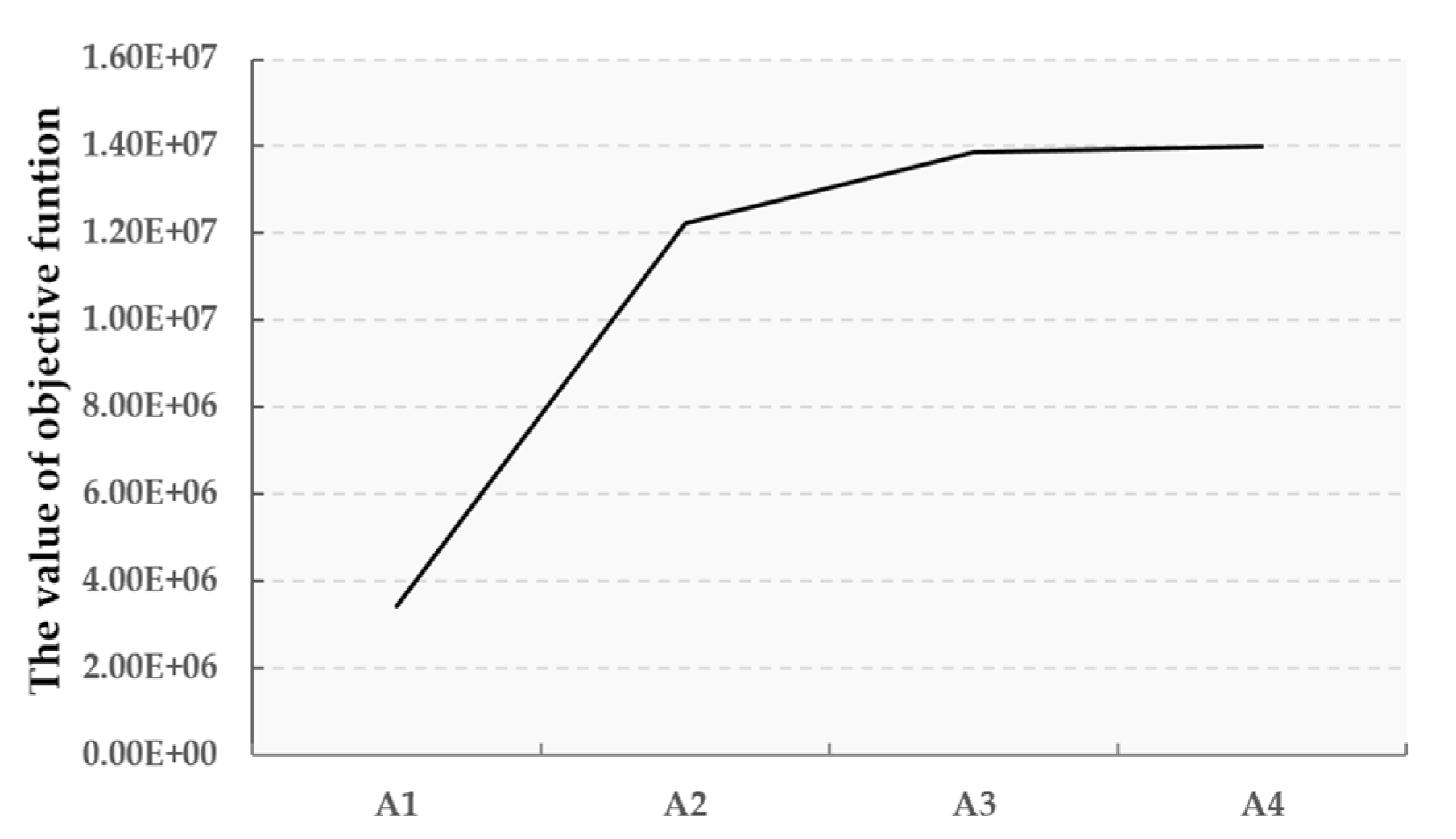
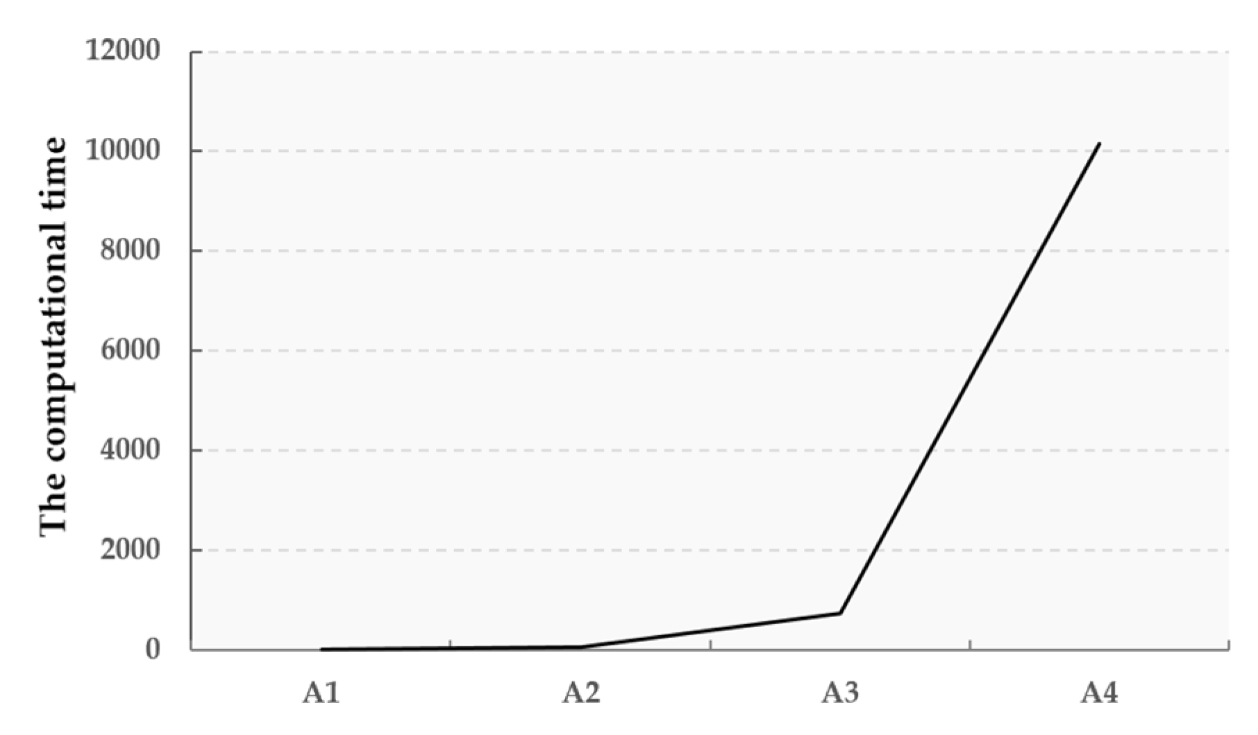
The structure of the train service network among reclassification yards remained unchanged. The values of objective functions and computational results of the four instances are listed in

Table 6. The computational results of four instances.

No.	Instance ID	Objective Function	Computational Time	Iterations	Satisfaction of Constraints
1	A1	3,428,402.00	17	75,764	√
2	A2	12,216,550.00	65	465,726	√
3	A3	13,855,090.00	734	3,446,840	√
4	A4	13,984,740.00	10,161	16,371,784	√

and depicted by Figure 7 and Figure 8, respectively.

The value of the objective function increased rapidly when adding the bulk shipment $N_{22}^{}$ into the network, while the iteration times increased significantly when four shipments were added into the network. The train formation plans of the four numerical instances are listed in

Table 7. The train formation plans of the four instances

No.	Instance ID	Direct Single- Commodity Train	Direct Multi- Commodity Train	Direct Train
1	A1	1 (S1→T1)	0	3 (K1→K5, K2→K5, K3→K5)
2	A2	2 (S1→T1, S1→T3)	0	3 (K1→K5, K2→K5, K3→K5)
3	A3	2 (S1→T1, S1→T3)	1 (S1→T3)	3 (K1→K5, K2→K5, K3→K5)
4	A4	2 (S1→T1, S1→T3)	1 (S1→T3)	3 (K1→K5, K2→K5, K3→K5)

.

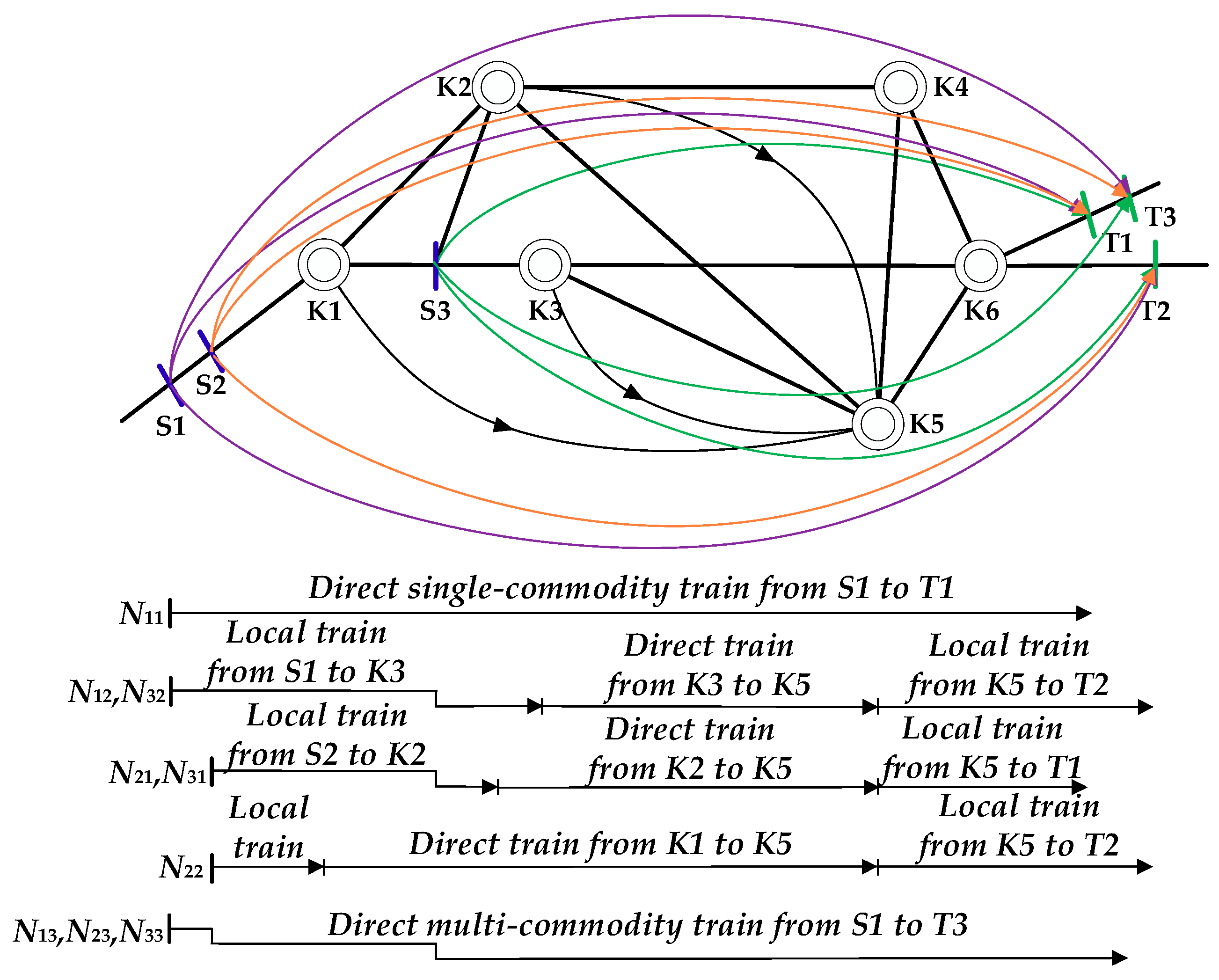
According to Table 7, a DMC train was operated when the carrying capacities of blocks were nearly full. This indicates that, if the traffic volumes of bulk shipments are not sufficient enough, it is actually more economical to add bulk shipments on direct trains instead of trains originating from the loading stations. The train formation plan for instance A4 is depicted in Figure 9.

The non-linear 0–1 programming model proposed in the present work can perfectly describe the actual and practical operations of railway systems. The branch-and-bound method employed was able to solve the model efficiently; however, there appeared a deficiency when solving relatively large-scale instances, which can in turn motivate subsequent research on linearization techniques and more ingenious solving methods.

6. Conclusions

In this paper, the train formation problem in loading stations was analyzed and formulated where a train service network among reclassification yards was pre-designed. One of the crucial preconditions of this work is that the loading and unloading equipment corresponding to specific categories of bulk commodities was symmetrical, which contributed to the symmetric loading and unloading efficiencies of one single bulk material. Furthermore, the supplies and distributions of the empty railcars to the loading stations and the symmetric distribution of loaded railcars to unloading stations were synchronous instead of respective.

Three train formation patterns were elaborated and discussed before modeling, including direct single-commodity trains, direct multi-commodity trains originating from loading stations, and direct trains from reclassification yards. The objective function was to minimize the total cost incurred by the loading, unloading, and reclassification operations on the basis of the classes of train formations. The non-linear programming model of the train formation problem in loading stations (TFLS) should also satisfy the pure strategy conditions, flow exclusive constraints, and logical relationships among decision variables. The commercial software Lingo was employed to solve the model, and an artificial case was carried out to illustrate the validity of the model and the effectiveness of the proposed method. This paper can be regarded as the foundation of the TFLS problem, and it can provide a theoretical support to design and optimize bulk train services in rail networks.

For future research, efficient linearization techniques corresponding to the non-linear forms in the TFLS problem can be the focus, such that the computational time can be reduced if a large-scale case is investigated. A set-partitioning model can be formulated for TFLS which can be compared to the compact formulation proposed in the present work (see Iris et al. [28]). Furthermore, a heuristic algorithm, such as the simulated annealing algorithm and particle swarm optimization, combined with the peculiarities of the TFLS problem, can be explored to improve the computational efficiency. Furthermore, the recoverable robustness of the train formation plan can be studied, and the relationship between recoverability and robustness is also a fascinating topic. Interested readers can refer to Iris and Lam [29]; in their study, the recoverable robustness was taken into consideration for the weekly berth and quay crane planning problem.

References

- European Commission. Roadmap to a Single European Transport Area—Towards a Competitive and Resource Efficient Transport System; White Paper: Brussels, Belgium, 2011. [Google Scholar]
- Three-Year Plan on Defending the Blue Sky issued by the State Council. Available online: http://www.gov.cn/zhengce/content/2018-07/03/content_5303158.htm (accessed on 30 September 2019).
- Martinelli, D.; Teng, H. Neural network approach for solving the train formation problem. Transp. Res. Board 1994, 1470, 38–46. [Google Scholar]
- Lin, B.; Wu, J.; Wang, J.; Duan, J.; Zhao, Y. A Bi-Level Programming Model for the Railway Express Cargo Service Network Design Problem. Symmetry 2018, 10, 227. [Google Scholar] [CrossRef]
- Bodin, L.D.; Golden, B.L.; Schuster, A.D.; Romig, W. A Model For the Blocking of Trains. Transp. Res. B-Meth. 1980, 14, 115–120. [Google Scholar] [CrossRef]
- Assad, A.A. Modelling of rail networks: Toward a routing/makeup model. Transp. Res. B-Meth. 1980, 14, 101–114. [Google Scholar] [CrossRef]
- Haghani, A.E. Formulation and solution of a combined train routing and makeup, and empty car distribution model. Transp. Res. B-Meth. 1989, 23, 433–452. [Google Scholar] [CrossRef]
- Crainic, T.; Ferland, J.; Rousseau, J.M. A Tactical Planning Model for Rail Freight Transportation. Transp. Sci. 1984, 18, 165–184. [Google Scholar] [CrossRef]
- Ahuja, R.K.; Jha, K.C.; Liu, J. Solving Real-Life Railroad Blocking Problems. Interfaces 2007, 37, 404–419. [Google Scholar] [CrossRef]
- Lin, B.L.; Wang, Z.M.; Ji, L.J.; Tian, Y.M.; Zhou, G.Q. Optimizing the freight train connection service network of a large-scale rail system. Transp. Res. B-Meth. 2012, 46, 649–667. [Google Scholar] [CrossRef]
- Cordeau, J.-F.; Toth, P.; Vigo, D. A Survey of Optimization Models for Train Routing and Scheduling. Transp. Sci. 1998, 32, 380–404. [Google Scholar] [CrossRef]
- Haghani, A.E. Rail freight transportation: A review of recent optimization models for train routing and empty car distribution. J. Adv. Transp. 1987, 21, 147–172. [Google Scholar] [CrossRef]
- Gorman, M.F.; Clarke, J.-P.; Gharehgozli, A.H.; Hewitt, M.; De Koster, R.; Roy, D. State of the Practice: A Review of the Application of OR/MS in Freight Transportation. INFORMS J. Appl. Anal. 2014, 44, 535–554. [Google Scholar] [CrossRef]
- Yaghini, M.; Sarmadi, M. Solving train formation problem using simulated annealing algorithm in a simplex framework. J. Adv. Transp. 2014, 48, 402–416. [Google Scholar] [CrossRef]
- Chen, C.; Dollevoet, T.; Zhao, J. One-block train formation in large-scale railway networks: An exact model and a tree-based decomposition algorithm. Transp. Res. Part B Methodol. 2018, 118, 1–30. [Google Scholar] [CrossRef] [Green Version]
- Xiao, J.; Pachl, J.; Lin, B.; Wang, J. Solving the block-to-train assignment problem using the heuristic approach based on the genetic algorithm and tabu search. Transp. Res. B-Meth. 2018, 108, 148–171. [Google Scholar] [CrossRef]
- Lin, B.L.; Zhu, S.N.; Shi, D.Y.; He, S.W. The optimal model of the direct train formation plan for loading area. China Railw. Sci. 1995, 16, 108–114. [Google Scholar]
- Cao, X.M.; Lin, B.L.; Yan, H.X. Optimization of direct freight train service in the loading place. China Railw. Soc. 2006, 28, 6–11. [Google Scholar]
- Fan, Z.; Lin, B.; Niu, H. Study on Nonstop Dr iving Scheme Depar ting from Loading Place. Log. Technol. 2008, 6, 77–80. [Google Scholar]
- Ji, L.; Lin, B.; Wang, Z. Study on the optimization of car flow organization for loading area based on logistics cost. China Railw. Soc. 2009, 31, 1–6. [Google Scholar]
- Masek, J.; Camaj, J.; Nedeliakova, E. Innovative Methods of Improving Train Formation in Freight Transport. Int. J. Mech. Aerosp. Ind. Mechatron. Manuf. Eng. 2015, 9, 1936–1939. [Google Scholar]
- Zhao, Y.; Lin, B. The Multi-Shipment Train Formation Optimization Problem Along the Ordered Rail Stations Based on Collection Delay. IEEE Access 2019, 7, 75935–75948. [Google Scholar] [CrossRef]
- Iris, Ç.; Christensen, J.; Pacino, D.; Ropke, S. Flexible ship loading problem with transfer vehicle assignment and scheduling. Transp. Res. B-Meth. 2018, 111, 113–134. [Google Scholar] [CrossRef] [Green Version]
- Holmberg, K.; Joborn, M.; Lundgren, J.T. Improved Empty Freight Car Distribution. Transp. Sci. 1998, 32, 163–173. [Google Scholar] [CrossRef]
- Joborn, M.; Crainic, T.G.; Gendreau, M.; Holmberg, K.; Lundgren, J.T. Economies of Scale in Empty Freight Car Distribution in Scheduled Railways. Transp. Sci. 2004, 38, 121–134. [Google Scholar] [CrossRef]
- Spieckermann, S.; Voß, S. A case study in empty railcar distribution. Eur. J. Oper. Res. 1995, 87, 586–598. [Google Scholar] [CrossRef]
- Newton, H.; Barnhart, C.; Vance, P. Constructing Railroad Blocking Plans to Minimize Handling Costs. Transp. Sci. 1998, 32, 330–345. [Google Scholar] [CrossRef]
- Iris, Ç.; Pacino, D.; Ropke, S.; Larsen, A. Integrated Berth Allocation and Quay Crane Assignment Problem: Set partitioning models and computational results. Transp. Res. E-Log. 2015, 81, 75–97. [Google Scholar] [CrossRef] [Green Version]
- Iris, Ç.; Lam, J.S.L. Recoverable robustness in weekly berth and quay crane planning. Transp. Res. B-Meth. 2019, 122, 365–389. [Google Scholar] [CrossRef]
Figure 1.
The loading vehicles of maritime navigation and railway transportation.
Figure 2.
An illustrative line rail network including three loading stations and two unloading stations.
Figure 3.
The alternative shipping strategies of bulk commodities in the loading stations. (a) Shipping strategy with four bulk train services; (b) Shipping strategy with three bulk train services; (c) Shipping strategy with three bulk train services; (d) Shipping strategy with two bulk train services; (e) Shipping strategy with two bulk train services and one train service; (f) Shipping strategy with two bulk train services and one train service.
Figure 4.
The artificial rail network and train services provided between yards. (a) The artificial rail network with bulk shipments; (b) The train service network.
Figure 5.
The train formation plan of the illustrative example.
Figure 6.
The extended rail network.
Figure 7.
The values of the objective function for the four numerical instances.
Figure 8.
The computational time for the four numerical instances.
Figure 9.
The train formation plan for instance A4.