Unsteady Flow of Fractional Fluid between Two Parallel Walls with Arbitrary Wall Shear Stress Using Caputo–Fabrizio Derivative

Abstract

In this article, unidirectional flows of fractional viscous fluids in a rectangular channel are studied. The flow is generated by the shear stress given on the bottom plate of the channel. The authors have developed a generalized model on the basis of constitutive equations described by the time-fractional Caputo–Fabrizio derivative. Many authors have published different results by applying the time-fractional derivative to the local part of acceleration in the momentum equation. This approach of the fractional models does not have sufficient physical background. By using fractional generalized constitutive equations, we have developed a proper model to investigate exact analytical solutions corresponding to the channel flow of a generalized viscous fluid. The exact solutions for velocity field and shear stress are obtained by using Laplace transform and Fourier integral transformation, for three different cases namely (i) constant shear, (ii) ramped type shear and (iii) oscillating shear. The results are plotted and discussed.

1. Introduction

The branch of mathematics that studies derivatives and integrals is called calculus, i.e., discussing integer order derivatives and integrals. When the order of derivatives changes from integer order to real (non-integer) order a new branch of calculus comes into being, called fractional calculus. Fractional order derivatives occur in many physical problems for example, frequency-dependent damping behavior of objects, velocity of infinite thin plate in a viscous fluid, creeping and relaxation functions of viscoelastic materials, and the control of dynamical systems as mentioned in [1,2,3,4]. Fractional calculus provides more generalized derivatives, and therefore it has more applications as compared with the classical or integer order derivatives. Fractional differential equations also explain the phenomena in electrochemistry, acoustics, electromagnetics, viscoelasticity, and material science [5,6,7,8,9,10]. For the last twenty years, a lot of work has been done on fractional calculus. Some authors [11,12,13] have used the formal definitions of fractional calculus like Riemann–Liouville and Caputo operators. These definitions provide a strong basis for the modern approach of Caputo and Fabrizio who have presented the definition without singular kernel [14].

The Caputo–Fabrizio differential operator is used by many authors to obtain exact solutions concerning real life problems [15,16,17]. All the benefits of Reimann–Liouville and Caputo definitions are also included in Caputo–Fabrizio, which is a worthy point of this definition. The Caputo–Fabrizio definition has been used by different authors in the medical sciences for example, the cancer treatment model and the flow of blood through veins under the effect of magnetic field [18,19]. Shah et al. [20] investigated the exact solutions over an isothermal vertical plate of free convectional flow of viscous fluids by using a definition of the Caputo–Fabrizio time-fractional derivative. Free convectional time-fractional flow with Newtonian heating near a vertical plate including mass diffusion has been investigated by Vieru et al. [21].

The effect of side walls over the velocity of a non-Newtonian fluid while the motion is produced due to the oscillation of the lower plate has been investigated by Fetecau et al. [22]. In addition, Haq et al. [23] have analyzed the exact solution of viscous fluid over an infinite plate using the Caputo–Fabrizio fractional order derivatives. Most of the authors have discussed different fluids using the fractional order differential operator defined by Caputo, Caputo–Fabrizio etc. and published many interesting results by applying the fractional order definition only to the local part of acceleration. Henry et al. [24] and Hristov [25,26] have suggested a generalized Fourier law for the thermal heat flux. It is clear from their discussion that the fractional differential operator has been employed in the constitutive relation of energy equation, rather than directly using it in the governing equation. This approach is appealing to mathematical and physical aspects of fluid mechanics. Hameid et al. [27] applied the definition of the fractional order derivative to the convective part of a constitutive equation and explained their model in a very interesting way. Vieru et al. [28] have followed the discussion presented by Hameid et al. [27] by applying the fractional derivative definition in a constitutive equation.

Keeping in mind all the above discussions, we present this article exploring the effect of side walls on the motion of an incompressible fluid using generalized fractional constitutive equations and the Caputo–Fabrizio derivative through a rectangular channel.

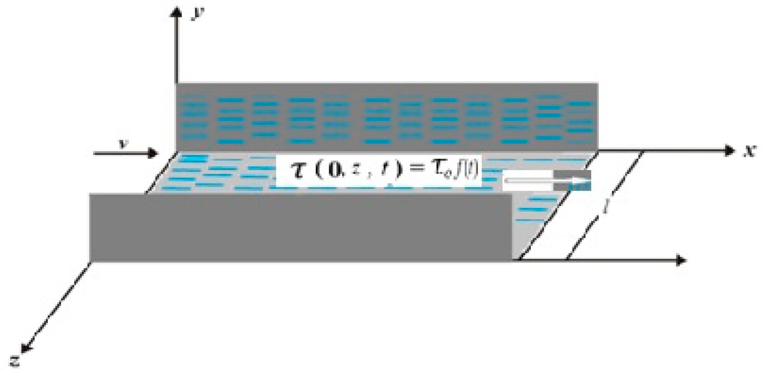
2. Problem Formulation

Consider an incompressible fluid, which is viscous in nature, present over an infinite plate between two parallel side walls that are at right angles to the horizontal plate as shown in Figure 1. Initially both the plate and fluid are at rest for t = 0, after time t > 0, and the flow is generated by the shear stress given by ${\tau }_{0}f(t)$ which engender the velocity as

$$\mathrm{V}=v(y,z,t)i,$$

(1)

where $i$ stands for unit vector.

In the absence of the body forces and the pressure gradient in the flow direction, the linear momentum equation in the x-direction is:

$$\rho \frac{\partial u_x}{\partial t}+u_x\frac{\partial u_x}{\partial x}+u_y\frac{\partial u_x}{\partial y}+u_z\frac{\partial u_x}{\partial z}=\frac{\partial {\tau }_{xy}}{\partial y}+\frac{\partial {\tau }_{xz}}{\partial z}$$

(2)

Therefore, in our case, the velocity field is the advection terms in Equation (2) that are zero with initial and boundary conditions as follows:

$$\begin{array}{l}v(y,z,0)=0,fory>0andz\in \left[0,l\right],\\ v(y,0,t)=v(y,l,t)=0fory,t>0,\\ {\tau }_{xy}(0,z,t)={\mu {}^{CF}D_t^{\alpha }\frac{\partial v(y,z,t)}{\partial y}|}_{y=0}={\tau }_{0}f(t),\end{array}$$

(3)

The above relation (Equation (3)), shows the shear stress which is non-trivial, where $\mu$ is dynamic viscosity, $\upsilon =\frac{\mu }{\rho },$ where ${\tau }_0$ shows the constant parameter, and it is assumed that $f(·)$ is a dimensionless, piecewise, continuous function such that $f(0)=0$, $v(y,z,t)$ and $\frac{\partial v(y,z,t)}{\partial y}\to 0asy\to \infty ,z\in [0,l]fort>0.$

We have the Caputo–Fabrizio derivative operator of order α given by Zafar et al. [29]

$${}^{CF}D_t^{\alpha }\left[h\left(t\right)\right]=\frac{1}{1-\alpha }{\displaystyle \underset{0}{\overset{t}{\int }}{h}^{\prime }(s)\exp \left[-\frac{\alpha (t-s)}{1-\alpha }\right]}ds\mathrm{for}0\le \alpha <1.$$

(4)

In the present paper, we consider the generalized constitutive equations with the Caputo–Fabrizio time-fractional derivative, namely:

$${\tau }_{xy}=\mu {}^{CF}D_t^{\alpha }\left(\frac{\partial v}{\partial y}\right)\mathrm{and}{\tau }_{xz}=\mu {}^{CF}D_t^{\alpha }\left(\frac{\partial v}{\partial z}\right)\mathrm{for}\alpha \in [0,1).$$

(5)

It is known that any constitutive equation must satisfy the principle of material objectivity, and therefore it must be frame-invariant with respect to Euclidean transformations. Yang et al. ([30], Equation (3.1)) have formulated a constitutive equation with fractional derivatives for generalized upper-convected Maxwell fluids on the basis of the convected coordinate system. They have proven that the proposed constitutive equation is frame-indifferent and have studied some particular cases of the proposed equation.

By applying the Laplace transform, the constitutive Equation (5) for the shear stress ${\tau }_{xy}$ can be written in the following equivalent form:

$${\tau }_{xy}=\frac{1}{1-\alpha }\frac{\partial v}{\partial y}-\frac{\alpha }{{\left(1-\alpha \right)}^2}{\displaystyle \underset{0}{\overset{t}{\int }}\exp \left(\frac{-\alpha (t-\tau )}{1-\alpha }\right)}\frac{\partial v(y,\tau )}{\partial y}d\tau ,0<\alpha <1.$$

(6)

Equation (6) is equivalent to the equation studied by Yang et al. ([30], Equation (4.5)), therefore, the proposed constitutive equations given by Equation (5) satisfy the principle of material objectivity.

3. Problem Solution

Using Equation (5) in Equation (2), applying Laplace transform to the obtained form and simplifying the result we get:

$$v(y,z,q)=\frac{\upsilon }{(1-\alpha )q+\alpha }\left[\frac{{\partial }^{2}v(y,z,q)}{\partial y^2}+\frac{{\partial }^{2}v(y,z,q)}{\partial z^2}\right],$$

(7)

where $v(y,z,q)={\displaystyle \underset{0}{\overset{\infty }{\int }}v(y,z,t)\exp (-qt)dt}$ is the Laplace transform with respect to t.

Applying the Fourier cosine transform with respect to variable y namely $v(\xi ,z,q)={\displaystyle \underset{0}{\overset{\infty }{\int }}v(y,z,q)\cos (y\xi )dy}$ and finite Fourier sine transform with respect to variable z $v(\xi ,n,q)={\displaystyle \underset{0}{\overset{l}{\int }}v(\xi ,z,q)\sin \left(\frac{n\pi z}{l}\right)dz,n=1,2,\dots }$, we obtain:

$$v_{sc}(\xi ,q)=\frac{\upsilon }{(1-\alpha )q+\alpha +\upsilon \left({\xi }^2+{{\lambda }_n}^2\right)}\frac{{\tau }_0}{\mu }\sqrt{\frac{2}{\pi }}f(q)\frac{{(-1)}^n-1}{{\lambda }_n},$$

(8)

where ${\lambda }_n=\frac{n\pi }{l}$ and subscript “sc” represents finite Fourier sine and inifinite cosine transforms.

For simplification, Equation (8) can be written as:

$$\begin{array}{ll}{v}_{sc}(\xi ,q)=\frac{{\tau }_0}{\mu }\frac{1-{(-1)}^n}{{\lambda }_n}\sqrt{\frac{2}{\pi }}\frac{f(q)}{\left({\xi }^2+{{\lambda }_n}^2\right)}-& \frac{{\tau }_0}{\mu }\frac{1-{(-1)}^n}{{\lambda }_n}\sqrt{\frac{2}{\pi }}f(q)\\ & \times \left[\frac{(1-\alpha )q+\alpha }{\left({\xi }^2+{{\lambda }_n}^2\right)\left[(1-\alpha )q+\alpha +\upsilon \left({\xi }^2+{{\lambda }_n}^2\right)\right]}\right]\end{array}.$$

(9)

Applying the inverse Laplace transformation, we get:

$$\begin{array}{ll}{v}_{sc}(\xi ,t)=\frac{{\tau }_0}{\mu }\sqrt{\frac{2}{\pi }}& \frac{1-{(-1)}^n}{{\lambda }_n}\frac{f(t)}{\left({\xi }^2+{{\lambda }_n}^2\right)}+\frac{1}{(1-\alpha )\left({\xi }^2+{{\lambda }_n}^2\right)}{\mathrm{e}}^{-A(\xi )t}\\ & \times \left[\frac{{\tau }_0}{\mu }\sqrt{\frac{2}{\pi }}\frac{1-{(-1)}^n}{{\lambda }_n}(1-\alpha )f^{•}(t)+\frac{{\tau }_0}{\mu }\sqrt{\frac{2}{\pi }}\frac{1-{(-1)}^n}{{\lambda }_n}\alpha f(t)\right]\end{array},$$

(10)

where $A(\xi )=\frac{\upsilon \left({\xi }^2+{{\lambda }_n}^2\right)+\alpha }{1-\alpha }$.

Applying the inverse Fourier transformation, we find:

$$v(y,z,t)=\frac{2}{\pi }\frac{2}{l}\frac{{\tau }_0}{\mu }{\displaystyle \sum _{n=1}^{\infty }\frac{{(-1)}^n-1}{{\lambda }_n}\sin ({\lambda }_{n}z)\left[\begin{array}{ll}f(t)\underset{0}{\overset{\infty }{\int }}\frac{\cos (y\xi )}{{\xi }^2+{{\lambda }_n}^2}d\xi +& \left[(1-\alpha )f^{•}(t)+\alpha f(t)\right]\\ & {\displaystyle \underset{0}{\overset{\infty }{\int }}\frac{\cos (y\xi )}{\left({\xi }^2+{{\lambda }_n}^2\right)}{e}^{-A(\xi )t}d\xi }\end{array}\right]},$$

(11)

where $m=2n-1$ and $l=2h$. Changing the origin by using z = z^* + h,

$$v(y,z,t)=\frac{2{\tau }_0}{\mu \pi h}{\displaystyle \sum _{n=1}^{\infty }\frac{{\left(-1\right)}^{n+1?}cos\left({\gamma }_m{z}^{*}\right)}{{\gamma }_m}\left[\begin{array}{ll}f(t)\underset{0}{\overset{\infty }{\int }}\frac{\cos (\mathrm{y}\xi )}{{\xi }^2+{{\gamma }_m}^2}d\xi +& \left[(1-\alpha )f^{•}(t)+\alpha f(t)\right]\\ & {\displaystyle \underset{0}{\overset{\infty }{\int }}\frac{\cos (\mathrm{y}\xi )}{\left({\xi }^2+{{\gamma }_m}^2\right)}{\mathrm{e}}^{-A(\xi )t}d\xi }\end{array}\right]}$$

(12)

ignoring the * notation, keeping in view the following result:

$${\displaystyle \underset{0}{\overset{\infty }{\int }}\frac{\cos (ax)}{b^2+x^2}dx=\frac{\pi }{2b}{\mathrm{e}}^{-ab},\mathrm{for}a>0\mathrm{Re}(b)>0},$$

and putting in Equation (11) we get:

$$\begin{array}{ll}v(y,z,t)=& \frac{2}{h}{\displaystyle \sum _{n=1}^{\infty }{(-1)}^{n+1}\frac{{\tau }_0}{\mu }\frac{\cos {\gamma }_{m}z}{{\gamma }_m}f(t)\frac{{\mathrm{e}}^{-y{\gamma }_m}}{{\gamma }_m}}-\frac{4}{\pi h}{\displaystyle \sum _{n=1}^{\infty }{(-1)}^{n+1}\frac{{\tau }_0}{\mu }\frac{\cos {\gamma }_{m}z}{{\gamma }_m}}\\ & \times \left[{\displaystyle \underset{0}{\overset{\infty }{\int }}{\displaystyle \underset{0}{\overset{t}{\int }}\frac{\cos (y\xi )}{{\xi }^2+{{\gamma }_m}^2}{f}^{•}(\mathrm{t}-\tau ){\mathrm{e}}^{-A(\xi )\tau }d\tau }d\xi }+\frac{\alpha }{1-\alpha }{\displaystyle \underset{0}{\overset{\infty }{\int }}{\displaystyle \underset{0}{\overset{t}{\int }}\frac{\cos (y\xi )}{{\xi }^2+{{\gamma }_m}^2}{f}^{•}(\mathrm{t}-\tau ){\mathrm{e}}^{-A(\xi )\tau }d\tau }d\xi }\right]\\ & \mathrm{where}{\gamma }_m=(2n-1)\frac{\pi }{2h}\end{array}.$$

(13)

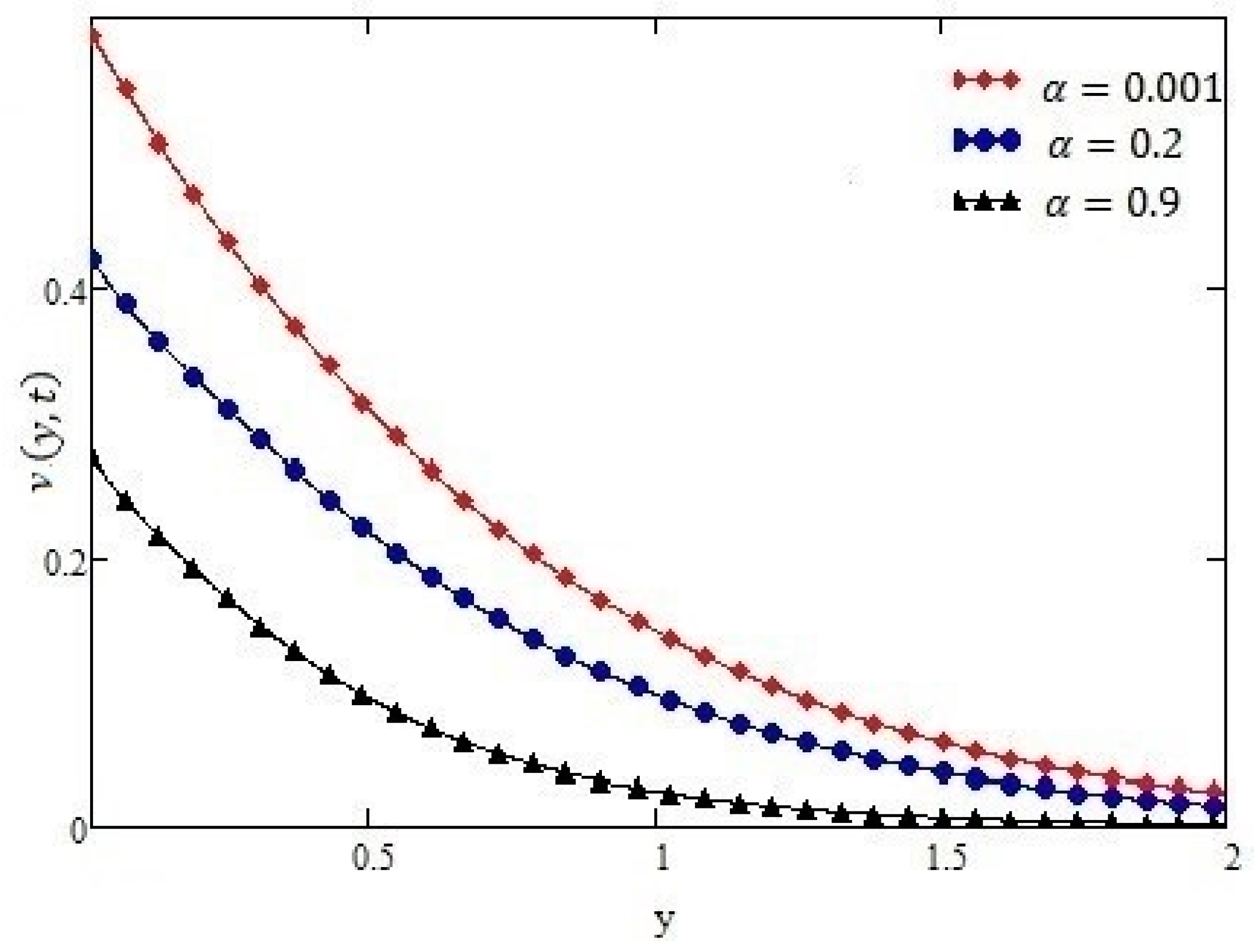
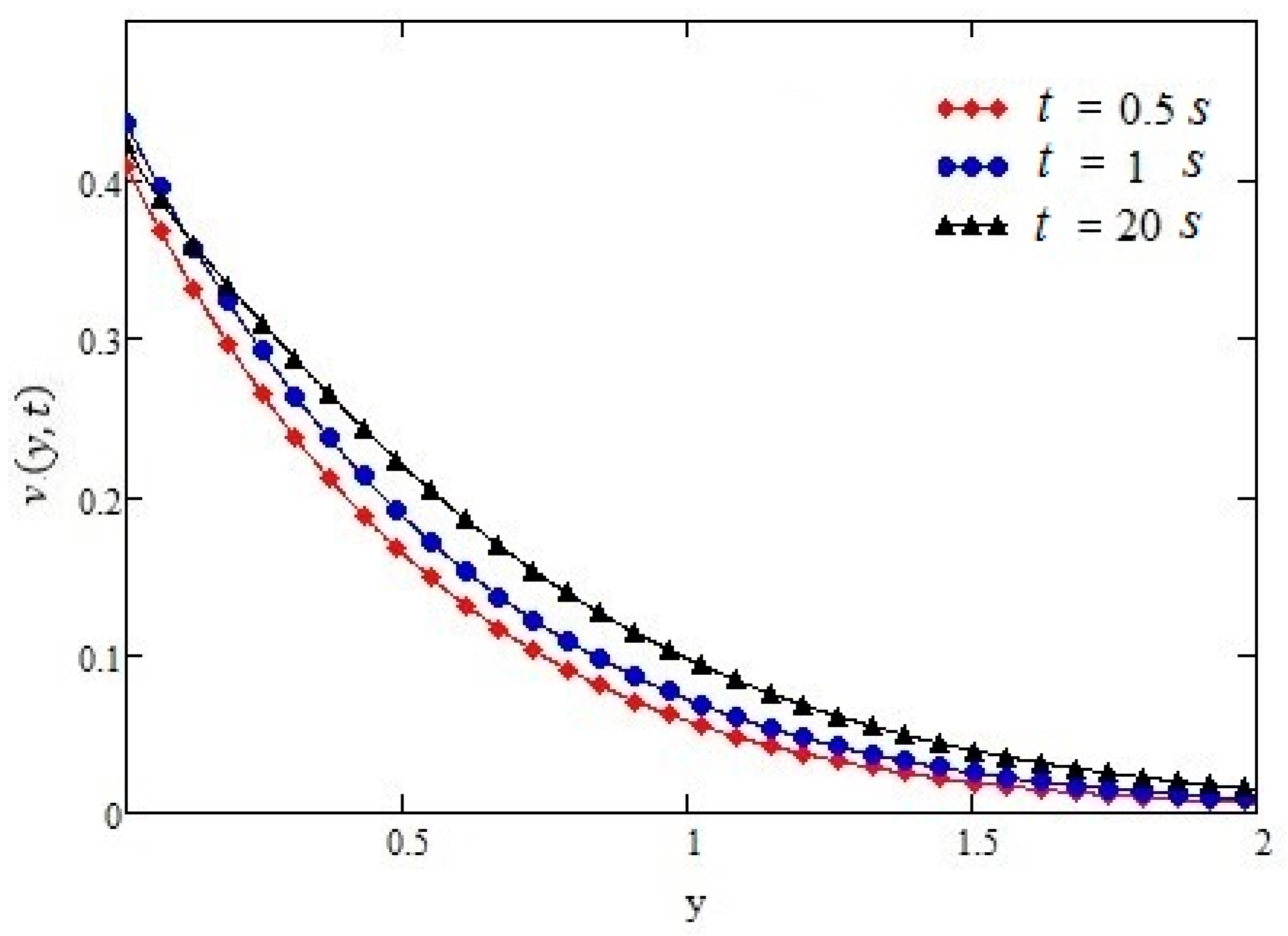
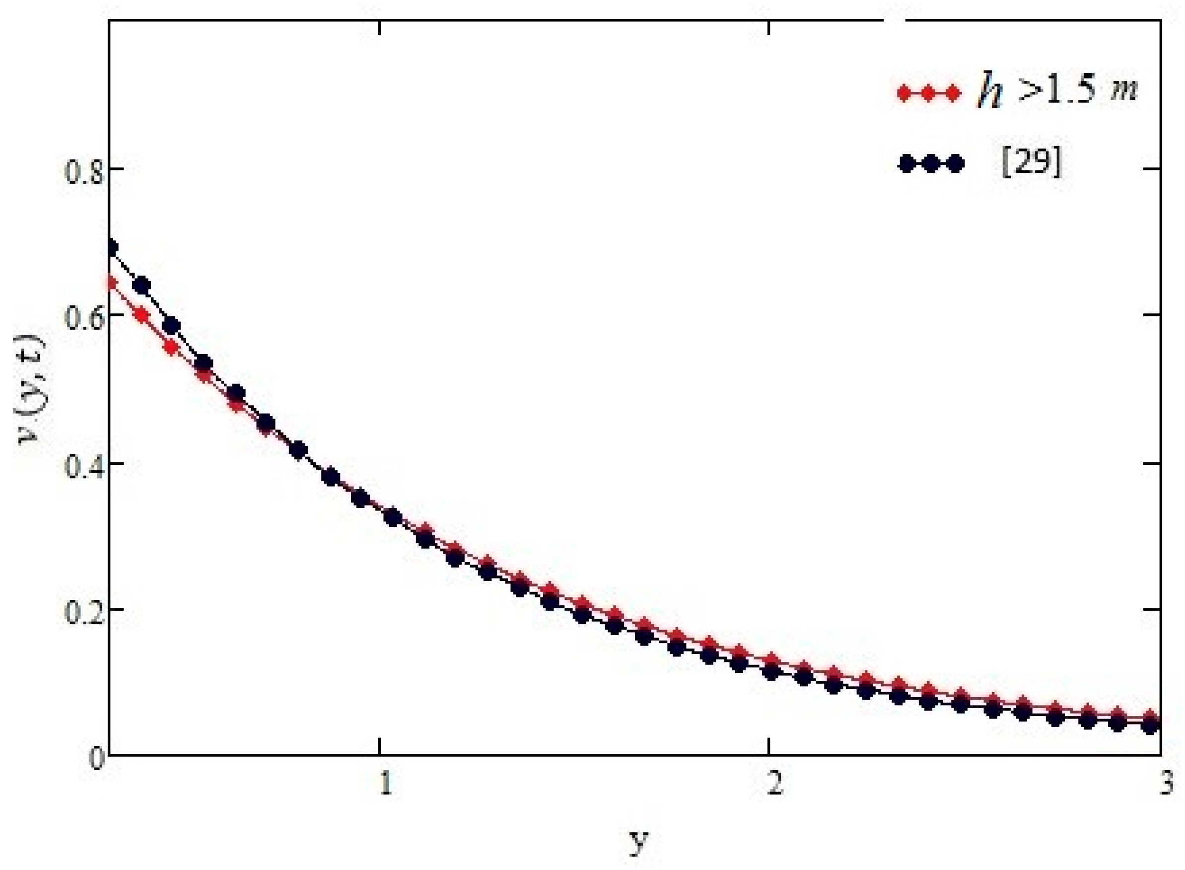
4. Graphical Illustration and Discussions

After finding the general solution for the velocity of the fluid, we discuss three different cases which are very useful in engineering. The obtained results are presented graphically for the three cases. Figure 2, Figure 3, Figure 4 and Figure 5 show different profiles of velocity by taking case I (constant shear) into consideration. Figure 6, Figure 7, Figure 8 and Figure 9 show the behavior of fluid velocity for case II (ramped type shear), and Figure 10, Figure 11 and Figure 12 show the same discussion for Case III (oscillating shear).

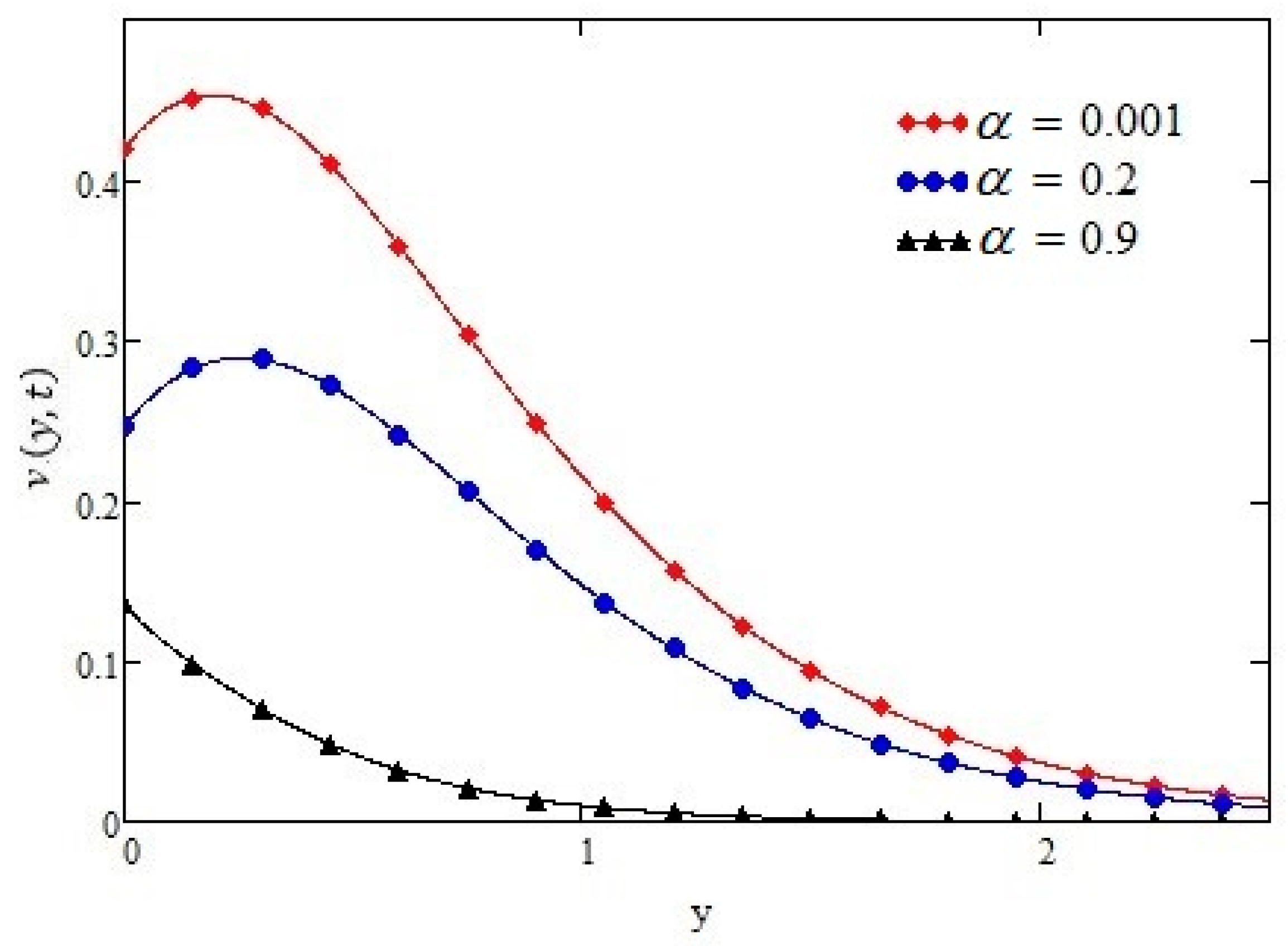
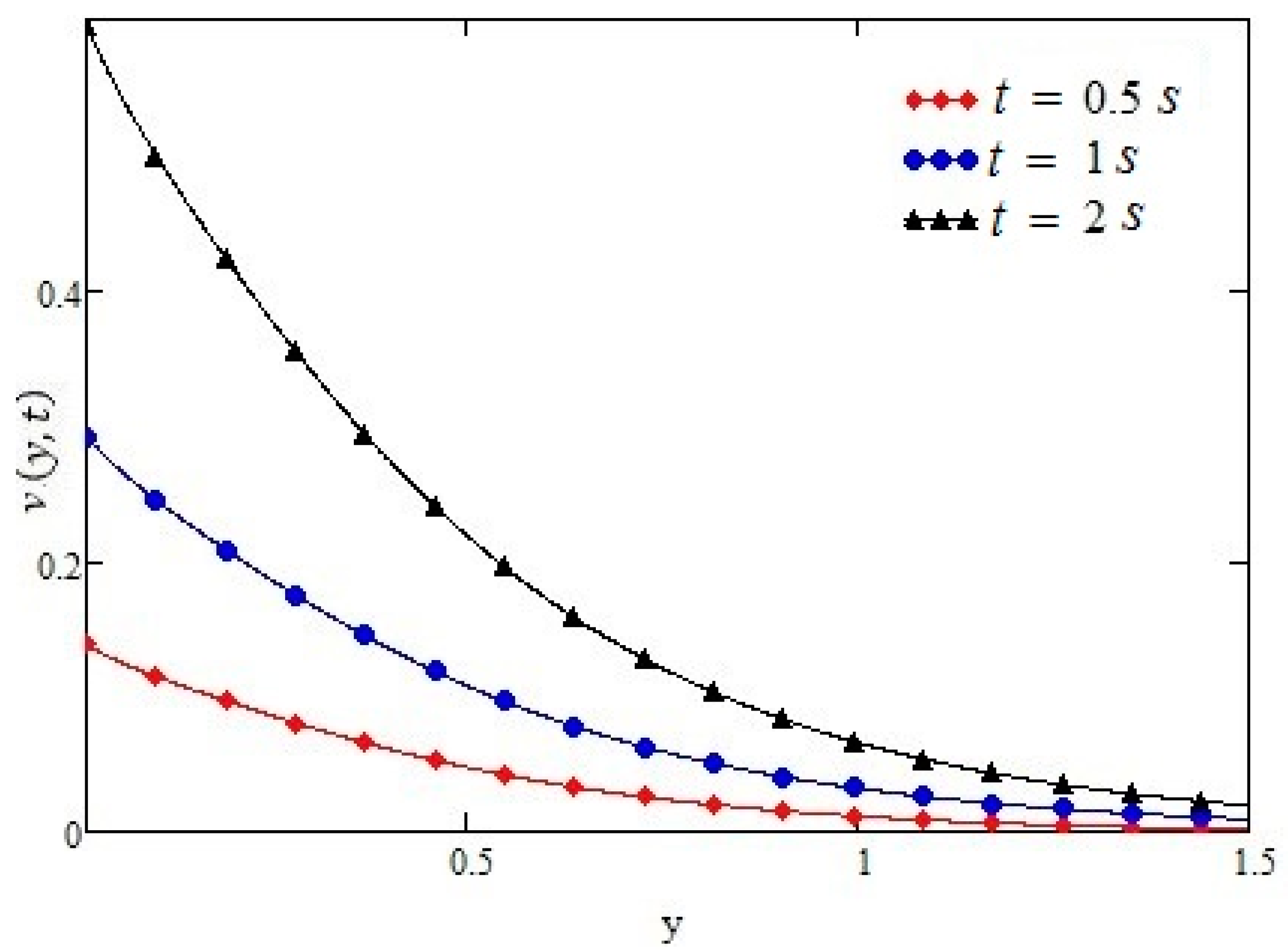
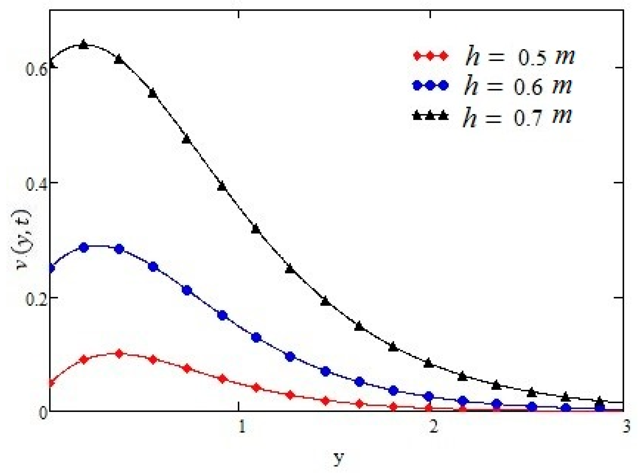
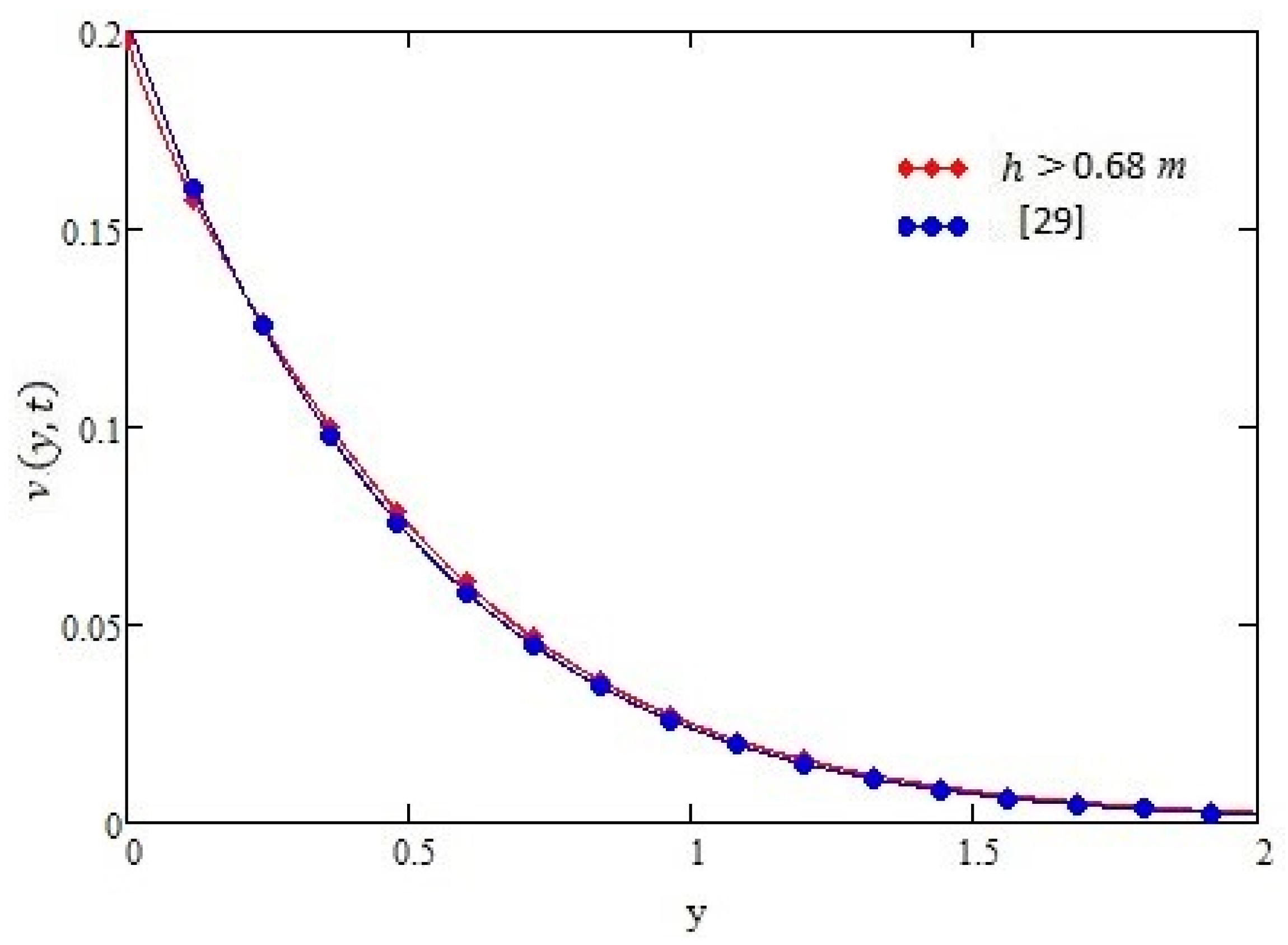
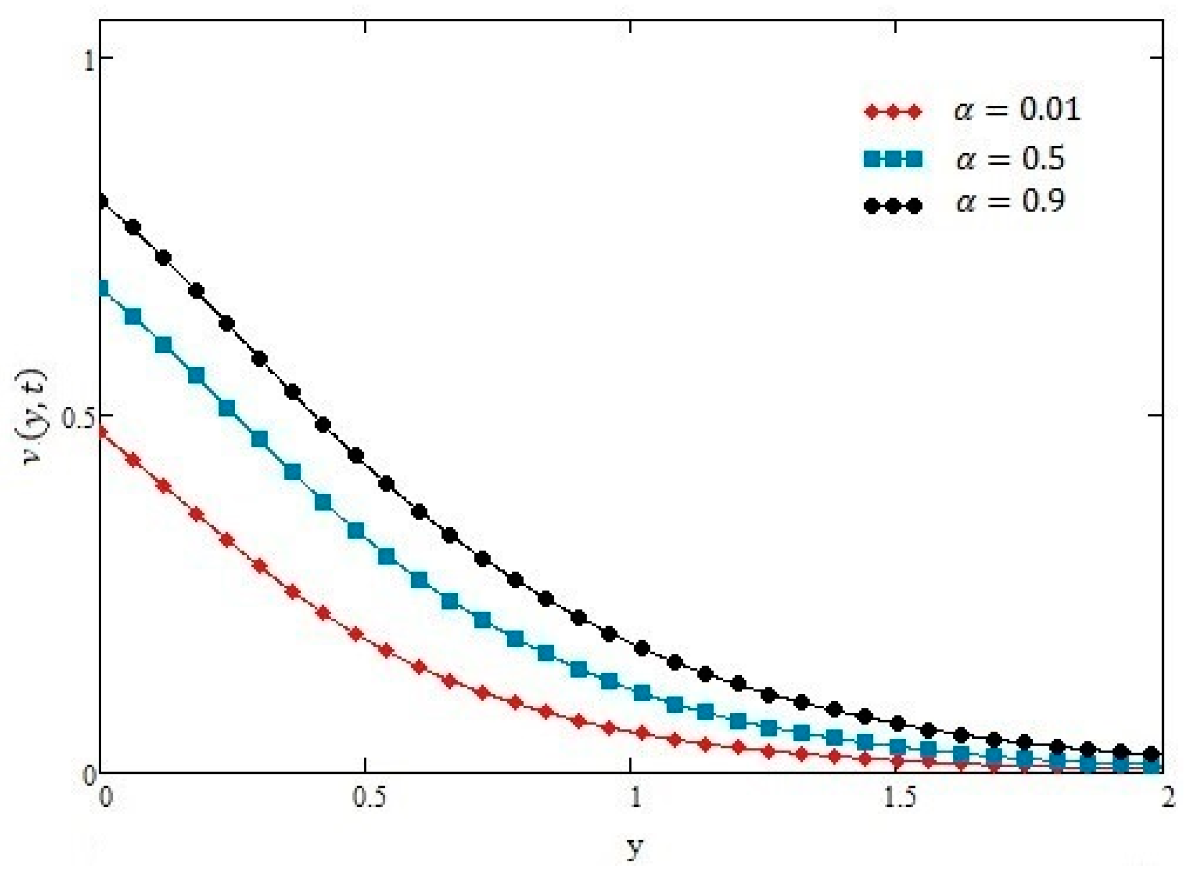
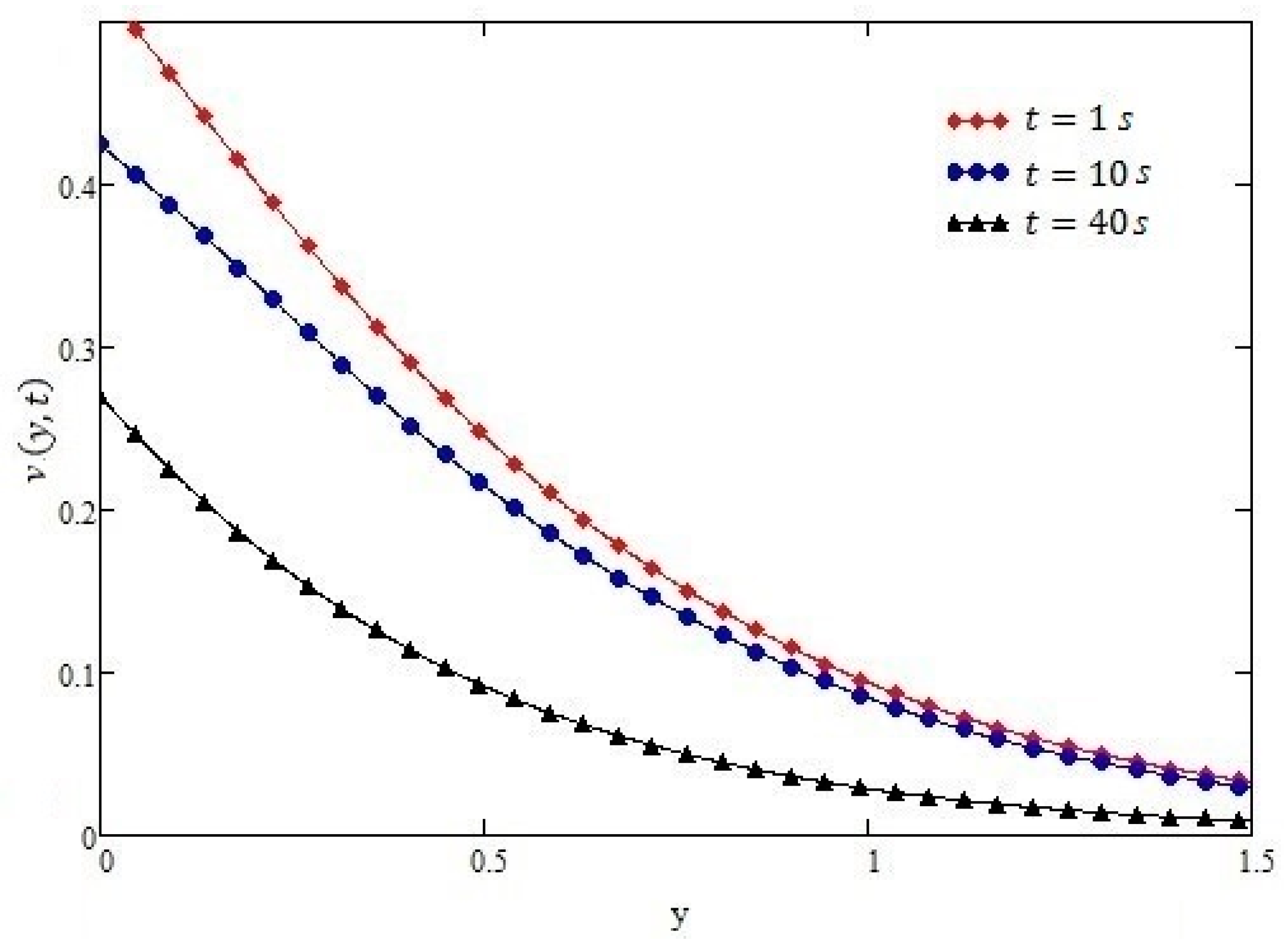
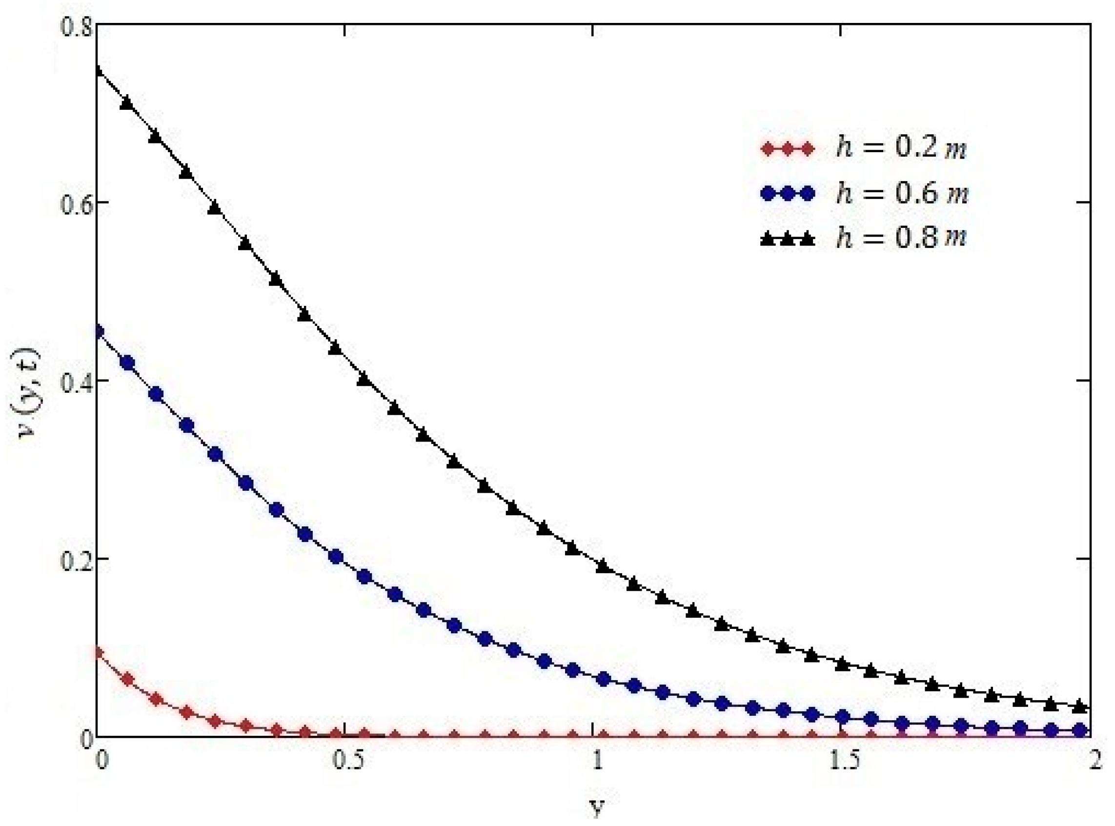
4.1. Case I (Constant Shear)

Taking $f(t)=H(t)$, where $H(t)$ is Heaviside unit step function we find the velocity profile as:

$$\begin{array}{ll}v(y,z,t)& =\frac{2}{h}{\displaystyle \sum _{n=1}^{\infty }{(-1)}^{n+1}}\frac{{\tau }_0}{\mu }\frac{\cos {\gamma }_{m}z}{{\gamma }_m}\left[\begin{array}{l}{\mathrm{e}}^{-y{\gamma }_m}+(1-\alpha )(t-\alpha )\\ \times {\mathrm{e}}^{-yA}\frac{B_n\cos (y{B}_n)+A_n\sin (y{B}_n)}{c_n\left(\sqrt{{b_n}^4+{c_n}^2}\right)}\end{array}\right]\\ & -\frac{4}{\pi h}{\displaystyle \sum _{n=1}^{\infty }{(-1)}^{n+1}}\frac{{\tau }_0}{\mu }\frac{\cos {\gamma }_{m}z}{{\gamma }_m}\left[{\displaystyle \underset{0}{\overset{\infty }{\int }}\left(\frac{{\mathrm{e}}^{-A(\xi )t}-1}{{(A(\xi ))}^2}-\frac{\alpha {\mathrm{e}}^{-A(\xi )t}}{(1-\alpha )A(\xi )}\right)\frac{\cos (y\xi )}{{\xi }^2+{{\gamma }_m}^2}d\xi }\right]\end{array},$$

(14)

Taking the following identity into account:

$${\displaystyle \underset{0}{\overset{\infty }{\int }}\frac{\cos (y\xi )}{{\left({\xi }^2-{b_n}^2\right)}^2+{c_n}^2}=\frac{\pi }{2c_n}{\mathrm{e}}^{-yA}}\frac{B_n\cos (y{B}_n)+A_n\sin (y{B}_n)}{\sqrt{{b_n}^4+{c_n}^2}},$$

where $2{A_n}^2=\sqrt{{b_n}^4+{c_n}^2}+{b_n}^2$ and $2{B_n}^2=\sqrt{{b_n}^4+{c_n}^2}-{b_n}^2$ in which: $b_n=\frac{\upsilon {{\gamma }_m}^2+\frac{\alpha }{2}}{\upsilon }\mathrm{and}{c}_n=\frac{\upsilon {{\gamma }_m}^4+\alpha {{\gamma }_m}^2}{\upsilon }-{b_n}^2$.

Figure 2 shows that as the value of α (0 < α < 1) is increasing, the fluid velocity is decreasing. Figure 3 shows the velocity profiles for different times, which implies that as time passages the fluid velocity increases in constant case. Figure 4 shows the profiles of velocity for different values of h, if we increase the distance between side walls the fluid velocity will increase while keeping the other parameters constant. Figure 5 shows the curve of Equation (14) is overlapping as that of [29] constant case if we increase the distance between the side walls to h ≥ 1.5, which gives our result for constant case more validity.

4.2. Case II (Ramped Type Shear)

Taking $f(t)=tH(t)$, we find the velocity profile as:

$$\begin{array}{ll}v(y,z,t)& =\frac{2}{d}{\displaystyle \sum _{n=1}^{\infty }{(-1)}^{n+1}}\frac{{\tau }_0}{\mu }\frac{\cos {\gamma }_{m}z}{{\gamma }_m}\frac{{\mathrm{e}}^{-y{\gamma }_m}}{{\gamma }_m}+\frac{2}{h}{\displaystyle \sum _{n=1}^{\infty }{(-1)}^{n+1}}\frac{{\tau }_0}{\mu }\frac{\cos {\gamma }_{m}z}{{\gamma }_m}\frac{{\mathrm{e}}^{-yA}}{c_n}\\ & \times \frac{B_n\cos (y{B}_n)+A_n\sin (y{B}_n)}{\left(\sqrt{{b_n}^4+{c_n}^2}\right)}\left[t(2-\alpha )-t^2(1-\alpha )\right]-\frac{4}{\pi h}{\displaystyle \sum _{n=1}^{\infty }{(-1)}^{n+1}}\\ & \times \frac{{\tau }_0}{\mu }\frac{\cos {\gamma }_{m}z}{{\gamma }_m}\left[{\displaystyle \underset{0}{\overset{\infty }{\int }}\left(2+\frac{\alpha }{(1-\alpha )}\right)}\frac{{\mathrm{e}}^{-A(\xi )t}}{A(\xi )}+\frac{1}{{\left(A(\xi )\right)}^2}\right]\frac{\cos (y\xi )}{{\xi }^2+{{\gamma }_m}^2}d\xi .\end{array}$$

(15)

Figure 6 shows that by increasing the value of the differential parameter the velocity of the fluid decreases. Figure 7 and Figure 8 show similar behavior of t and h, as observed in Figure 3 and Figure 4, whereas in Figure 9, we calculated the value of h in order to validate our result in case of ramped type shear.

4.3. Case III (Oscillating Shear Stress)

Taking $f(t)=\sin (\omega t)H(t)$, in Equation (13) we get the velocity profile as:

$$\begin{array}{ll}v(\mathrm{y},\mathrm{z},\mathrm{t})& ={\displaystyle \sum _{n=1}^{\infty }{(-1)}^{n+1}\frac{{\tau }_0}{\mu }}\frac{\cos {\gamma }_{m}z}{{\gamma }_m}[\frac{2}{h}\sin (\omega \mathrm{t})\frac{{\mathrm{e}}^{-y{\gamma }_m}}{{\gamma }_m}-\frac{4}{\pi h}{\displaystyle \underset{0}{\overset{\infty }{\int }}\{\frac{1}{{\left(A(\xi )\right)}^2+{\omega }^2}}\\ & \times (-A(\xi ){\mathrm{e}}^{-A(\xi )t}+A(\xi )\cos (\omega t)+\omega \sin (\omega t)+\frac{\alpha }{1-\alpha }\\ & \times (\omega {\mathrm{e}}^{-A(\xi )t}+\omega \cos (\omega \mathrm{t})+A(\xi )\sin (\omega \mathrm{t})))\}\frac{\cos (y\xi )}{{\xi }^2+{{\gamma }_m}^2}d\xi ].\end{array}$$

(16)

Figure 10 and Figure 11 show opposite behavior as compared to those of constant and ramped type shear for α and time t parameters, and Figure 12 shows the same behavior as the previous two cases for parameter h, i.e., distance between side walls.

5. Conclusions

This article is presented to obtain the exact solution in general form for the velocity of the fluid present over an infinite plate between two side walls using the definition of the Caputo–Fabrizio of fractional order differential operator, while the motion is produced due to shear stress as τ₀f(t). The results are obtained by using Laplace and Fourier transformations for three different cases:

• Constant shear;
• Ramped type shear;
• Oscillating shear.

After the above discussion we have concluded the following results.

Firstly, keeping the condition on shear the response of the fractional fluid velocity is very quick, as compared with that of ordinary fluid velocity for all the cases. Secondly, in fractional fluid a small change in time parameter shows a clear difference for the profiles in all the cases listed above. Thirdly, for the above cases there are some values of h at which the motion of the fluid is unaffected by side walls.

References

1. Podlubny, I. Fractional Differential Equations: An Introduction to Fractional Derivatives, Fractional Differential Equations, to Methods of Their Solution and Some of Their Applications; Elsevier: Amsterdam, The Netherlands, 1998; Volume 198. [Google Scholar]
2. Torvik, P.J.; Bagley, R.L. On the appearance of the fractional derivative in the behavior of real materials. J. Appl. Mech. 1984, 51, 294–298. [Google Scholar] [CrossRef]
3. Caputo, M. Elasticità e dissipazione; Zanichelli: Bologna, Italy, 1969. [Google Scholar]
4. Suarez, L.; Shokooh, A. An eigenvector expansion method for the solution of motion containing fractional derivatives. J. Appl. Mech. 1997, 64, 629–635. [Google Scholar] [CrossRef]
5. Michalski, M.W. Derivatives of Noninteger Order and Their Applications; Institute of Mathematics, Polish Academy of Sciences Warsaw: Warszawa, Poland, 1993. [Google Scholar]
6. Gloeckle, W.G.; Nonnenmacher, T.F. Fractional integral operators and fox functions in the theory of viscoelasticity. Macromolecules 1991, 24, 6426–6434. [Google Scholar] [CrossRef]
7. Ray, S.S.; Bera, R. An approximate solution of a nonlinear fractional differential equation by adomian decomposition method. Appl. Math. Comput. 2005, 167, 561–571. [Google Scholar]
8. Babenko, Y. Non integer differential equation. In Proceedings of the 3rd International Conference on Intelligence in Networks, Bordeaux, France, 11–13 October 1994. [Google Scholar]
9. Gaul, L.; Klein, P.; Kemple, S. Damping description involving fractional operators. Mech. Syst. Signal Process. 1991, 5, 81–88. [Google Scholar] [CrossRef]
10. Ochmann, M.; Makarov, S. Representation of the absorption of nonlinear waves by fractional derivatives. J. Acoust. Soc. Am. 1993, 94, 3392–3399. [Google Scholar] [CrossRef]
11. Kumar, S. A new fractional modeling arising in engineering sciences and its analytical approximate solution. Alex. Eng. J. 2013, 52, 813–819. [Google Scholar] [CrossRef] [Green Version]
12. Mainardi, F. Fractional Calculus and Waves in Linear Viscoelasticity: An Introduction to Mathematical Models; World Scientific: Singapore, 2010. [Google Scholar]
13. Podlubny, I.; Chechkin, A.; Skovranek, T.; Chen, Y.; Jara, B.M.V. Matrix approach to discrete fractional calculus ii: Partial fractional differential equations. J. Comput. Phys. 2009, 228, 3137–3153. [Google Scholar] [CrossRef]
14. Caputo, M.; Fabrizio, M. A new definition of fractional derivative without singular kernel. Progr. Fract. Differ. Appl. 2015, 1, 1–13. [Google Scholar]
15. Atangana, A. On the new fractional derivative and application to nonlinear fishers reaction–diffusion equation. Appl. Math. Comput. 2016, 273, 948–956. [Google Scholar]
16. Caputo, M.; Fabrizio, M. Applications of new time and spatial fractional derivatives with exponential kernels. Progr. Fract. Differ. Appl. 2016, 2, 1–11. [Google Scholar] [CrossRef]
17. Fetecau, C.; Vieru, D.; Fetecau, C.; Akhter, S. General solutions for magnetohydrodynamic natural convection flow with radiative heat transfer and slip condition over a moving plate. Z. Naturforsch. A 2013, 68, 659–667. [Google Scholar] [CrossRef]
18. Dokuyucu, M.A.; Celik, E.; Bulut, H.; Baskonus, H.M. Cancer treatment model with the caputo-fabrizio fractional derivative. Eur. Phys. J. Plus 2018, 133, 92. [Google Scholar] [CrossRef]
19. Riaz, M.; Zafar, A. Exact solutions for the blood flow through a circular tube under the influence of a magnetic field using fractional caputo-fabrizio derivatives. Math. Model. Nat. Phenom. 2018, 13, 8. [Google Scholar] [CrossRef]
20. Shah, N.A.; Imran, M.; Miraj, F. Exact solutions of time fractional free convection flows of viscous fluid over an isothermal vertical plate with caputo and caputo-fabrizio derivatives. J. Prime Res. Math. 2017, 13, 56–74. [Google Scholar]
21. Vieru, D.; Fetecau, C.; Fetecau, C. Time-fractional free convection flow near a vertical plate with newtonian heating and mass diffusion. Therm. Sci. 2015, 19 (Suppl. 1), 85–98. [Google Scholar] [CrossRef]
22. Fetecau, C.; Vieru, D.; Fetecau, C. Effect of side walls on the motion of a viscous fluid induced by an infinite plate that applies an oscillating shear stress to the fluid. Cent. Eur. J. Phys. 2011, 9, 816–824. [Google Scholar] [CrossRef] [Green Version]
23. Haq, S.U.; Khan, M.A.; Shah, N.A. Analysis of magneto hydrodynamic flow of a fractional viscous fluid through a porous medium. Chin. J. Phys. 2018, 56, 261–269. [Google Scholar] [CrossRef]
24. Henry, B.I.; Langlands, T.A.; Straka, P. An introduction to fractional diffusion. In Complex Physical, Biophysical and Econophysical Systems; World Scientific: Singapore, 2010; pp. 37–89. [Google Scholar]
25. Hristov, J. Transient heat diffusion with a non-singular fading memory: From the cattaneo constitutive equation with jeffreys kernel to the caputofabrizio time-fractional derivative. Therm. Sci. 2016, 20, 757–762. [Google Scholar] [CrossRef]
26. Hristov, J. Derivatives with non-singular kernels from the caputo–fabrizio definition and beyond: Appraising analysis with emphasis on diffusion models. Front. Fract. Calc. 2017, 1, 270–342. [Google Scholar]
27. El-Lateif, A.M.A.; Abdel-Hameid, A.M. Comment on “solutions with special functions for time fractional free convection flow of brinkman-type fluid” by F. Ali et al. Eur. Phys. J. Plus 2017, 132, 407. [Google Scholar] [CrossRef]
28. Ahmed, N.; Shah, N.A.; Vieru, D. Natural convection with damped thermal flux in a vertical circular cylinder. Chin. J. Phys. 2018, 56, 630–644. [Google Scholar] [CrossRef]
29. Zafar, A.; Fetecau, C. Flow over an infinite plate of a viscous fluid with noninteger order derivative without singular kernel. Alex. Eng. J. 2016, 55, 2789–2796. [Google Scholar] [CrossRef]
30. Yang, P.; Lam, Y.C.; Zhu, K.Q. Constitutive equation with fractional derivatives for the generalized UCM model. J. Non-Newton. Fluid Mech. 2010, 165, 88–97. [Google Scholar] [CrossRef]
Figure 1. Geometry of the problem.
Symmetry 11 00449 g001
Figure 2. Profiles of velocity given by Equation (14) of constant shear for different values of α, for t = 20 s, h = 0.6 m, τ0 = −1 N/m2, ν = 0.1 m2/s, and µ = 1.4 kg·m/s.
Symmetry 11 00449 g002
Figure 3. Profiles of velocity given by Equation (14) of constant shear for different values of t, for α = 0.2, h = 0.6 m, τ0 = −1 N/m2, ν = 0.1 m2/s, and µ = 1.4 kg·m/s.
Symmetry 11 00449 g003
Figure 4. Profiles of velocity given by Equation (14) of constant shear for different values of h, for t = 0.5 s, α = 0.2, τ0 = −1 N/m2, ν = 0.1 m2/s, and µ = 1.4 kg·m/s.
Symmetry 11 00449 g004
Figure 5. The value of h required for overlapping the velocity profiles of equation (14) and infinite plate [29] in constant shear for t = 0.5 s, α = 0.2, τ0 = −1 N/m2, ν = 0.1 m2/s, µ = 1.4 kg·m/s, and h > 1.5 m.
Symmetry 11 00449 g005
Figure 6. Profiles of velocity given by Equation (15) of ramped type shear velocity for different values of α, for t = 0.5 s, h = 0.6 m, τ0 = −1 N/m2, ν = 0.1 m2/s, and µ = 1.4 kg·m/s.
Symmetry 11 00449 g006
Figure 7. Profiles of velocity given by Equation (15) of ramped type shear for different values of t, for α = 0.9, h = 0.6 m, τ0 = −1 N/m2, ν = 0.1 m2/s, and µ = 1.4 kg·m/s.
Symmetry 11 00449 g007
Figure 8. Profiles of velocity given by Equation (15) of ramped type shear for different values of h, for t = 0.5 s, α = 0.2, τ0 = −1 N/m2, ν = 0.1 m2/s, and µ = 1.4 kg·m/s.
Symmetry 11 00449 g008
Figure 9. The value of h required for overlapping the velocity profiles of Equation (15) and infinite plate [29] in ramped type shear for t = 0.4 s, α = 0.9, ν = 0.1 m2/s, τ0 = −1.5 N/m2, µ = 1.4 kg·m/s and h ≥ 0.68.
Symmetry 11 00449 g009
Figure 10. Profiles of velocity given by Equation (16) of oscillating shear for different values of α, for t = 1 s, h = 0.6 m, ν = 0.05 m2/s, τ0 = −1 N/m2, µ = 1.4 kg·m/s, and ω = 1.
Symmetry 11 00449 g010
Figure 11. Profiles of velocity given by Equation (16) of oscillating shear for different values of t, for α = 0.5, h = 0.6 m, τ0 = −1 N/m2, ν = 0.1 m2/s, µ = 1.4 kg·m/s, and ω = 1.
Symmetry 11 00449 g011
Figure 12. Profiles of velocity given by Equation (16) of oscillating shear for different values of h, for t = 1 s, α = 0.5, τ0 = −1 N/m2, ν = 0.1 m2/s, µ = 1.4 kg·m/s, and ω = 1.
Symmetry 11 00449 g012