Some Picture Fuzzy Dombi Heronian Mean Operators with Their Application to Multi-Attribute Decision-Making

Abstract

As an extension of the intuitionistic fuzzy set (IFS), the recently proposed picture fuzzy set (PFS) is more suitable to describe decision-makers’ evaluation information in decision-making problems. Picture fuzzy aggregation operators are of high importance in multi-attribute decision-making (MADM) within a picture fuzzy decision-making environment. Hence, in this paper our main work is to introduce novel picture fuzzy aggregation operators. Firstly, we propose new picture fuzzy operational rules based on Dombi t-conorm and t-norm (DTT). Secondly, considering the existence of a broad and widespread correlation between attributes, we use Heronian mean (HM) information aggregation technology to fuse picture fuzzy numbers (PFNs) and propose new picture fuzzy aggregation operators. The proposed operators not only fuse individual attribute values, but also have a good ability to model the widespread correlation among attributes, making them more suitable for effectively solving increasingly complicated MADM problems. Hence, we introduce a new algorithm to handle MADM based on the proposed operators. Finally, we apply the newly developed method and algorithm in a supplier selection issue. The main novelties of this work are three-fold. Firstly, new operational laws for PFSs are proposed. Secondly, novel picture fuzzy aggregation operators are developed. Thirdly, a new approach for picture fuzzy MADM is proposed.

1. Introduction

Decision-making science is an ancient and dynamic discipline. In daily life and the management of companies, we often encounter decision-making problems. For example, an enterprise has to select a most suitable supplier to gain a stable supply channel. Investment companies need to choose a suitable investment project to achieve stable returns. An airline company needs to evaluate existing routes to get the best one and calls others to learn about the route. In the past decades, research on decision-making methods has attracted scholars’ interest in both theoretical and practical aspects [1,2,3,4,5,6]. Moreover, due to the complexity of decision-making problems, in most real-life decision-making issues alternatives have to be evaluated from multiple perspectives instead of only one before determining the most suitable alternative. Thus, multi-attribute decision-making (MADM) models have attracted the attention of many scholars [7,8,9,10,11,12,13,14,15]. Nevertheless, expressing decision-makers’ decision information and representing attribute values in MADM are always a huge challenge due to some reasons. The high complexity of practical decision-making problems lead to the difficulties of representing attribute values properly. Secondly, influenced by subjective factors such as decision-makers’ own experience, cognitive ability and intuition, it is often difficult for decision-makers to access all decision information. Thus, representing attribute values appropriately and correctly is urgently required. Recently, many scholars have been dedicated to investigating tools and methods that can describe uncertain information and quite a few influential theories have been proposed. Zadeh [16] originally provided an effective tool, called fuzzy set (FS), to deal with fuzziness and ambiguity. Since its introduction, FS has received widespread attention in academia. Afterwards, Atanassov [17] pointed out the defects of FSs and proposed an extension, called intuitionistic fuzzy set (IFS), which describes uncertain phenomena and information from both membership and non-membership degrees. As IFSs have obvious advantages in describing uncertain information and data, they have drawn much attention among scholars. Xu [18] and Xu and Yager [19] introduced intuitionistic fuzzy simple weighted average operators. Based on the Einstein t-conorm and t-norm, Wang and Liu [20] and Zhang [21] proposed a series of intuitionistic fuzzy Einstein aggregation operators. To capture the interrelationship between intuitionistic fuzzy numbers (IFNs), Xu and Yager [22] and Xia [23] proposed intuitionistic fuzzy Bonferroni mean operators and their generalized forms, respectively. Qin and Li [24] proposed intuitionistic fuzzy Maclaurin symmetric mean operators in order to reflect interrelationships among multiple attributes. More work about IFSs in decision-making can be found in the literature [25,26,27,28,29,30,31,32,33,34].

IFSs have good ability to describe and express decision-makers’ fuzzy decision information in MADM problems. Nevertheless, IFS still have drawbacks and there exist quite a few circumstances in which it is improper to use IFS to express decision-makers’ preference information. The main reason is that the indeterminacy degree is a default in IFSs, for example when a decision-maker uses an IFN (0.3, 0.4) to denote his/her evaluation on a certain attribute. Then, the indeterminacy degree of the decision-maker is 1 − 0.3 − 0.4 = 0.3. In other words, once the membership and non-membership degrees are determined, the degree of indeterminacy is determined automatically. However, this is quite different from actual MADM problems. In practical MADM, the indeterminacy degrees should not be determined automatically and should be provided by decision-makers. For instance, if a decision-maker thinks the membership degree is 0.2, the membership degree is 0.3, and the degree that he/she is not sure about the result is 0.1, then the decision-maker’s evaluation value can be denoted as (0.2, 0.1, 0.3), which cannot be represented by IFSs. In order to deal with this case, Cuong [35] proposed the concept of picture fuzzy set (PFS), characterized by a positive membership degree, a neutral membership degree, and a negative membership degree. Owing to their great power to heal the inherent fuzziness of information, Le et al. [36] incorporated IFSs into fuzzy inference systems to enhance their performance. Le [37] proposed generalized picture distance measure and integrate it to a novel hierarchical picture fuzzy clustering method, called hierarchical picture clustering. Owing to PFSs’ high capacity to model fuzziness, they also have been widely applied in MADM [38,39,40,41,42,43,44]. Generally speaking, there are two types of MADM method. The first type is based on traditional decision-making methods. In other words, the traditional methods are extended to accommodate MADM with picture fuzzy information. Another type is from the aggregation operators’ point of view. Aggregation operators can integrate attribute values into a collective values and select the optimal alternative accordingly. To effectively aggregate picture fuzzy information, a mass of picture fuzzy aggregation operators have been put forward for aggregating PFNs [45,46,47,48]. Although these operators have been successfully applied in picture fuzzy MADM, there are still some limits. First of all, all the aforementioned picture fuzzy operators are based on algebraic operational laws for PFNs. Thus, Wei [49] proposed some picture fuzzy Hamacher aggregation operators based on Hamacher t-norm and t-conorm. The recently proposed Dombi t-conorm and t-norm (DTT) [50] are powerful in information aggregation and, recently, have been applied to the aggregation process of intuitionistic fuzzy information [51], hesitant fuzzy information [52], and single-valued neutrosophic information [53]. However, Dombi t-conorm and t-norms have not been applied to the aggregation of PFNs. Therefore, it is necessary to extend Dombi t-conorm and t-norms to PFNs and propose new operational laws of PFNs. Secondly, all the picture fuzzy aggregation operators do not consider the interrelationship among PFNs. However, attributes in most real MADM problems are correlated, meaning the interrelationship between attribute values should be considered when aggregating them. Recently, a number of information aggregation tools that can consider such interrelationships among aggregated variables have been raised to a model, such as the Bonferroni mean (BM) [54] and Heronian mean (HM) [55]. In existing literature [56], scholars have analyzed how HM has some meliority over BM. Hence, this paper uses HM as the essential information aggregation method to fuse PFNs on the basis of DTT. Furthermore, we propose a new method for MADM within the scope of PFSs.

The motivations and contributions of this paper are (1) to propose some new operations for PFNs based on DTT; (2) to propose some picture fuzzy Dombi Heronian mean operators to aggregate PFNs; and (3) to propose a novel approach to MADM. In order to do this, the remainder of this paper is organized as follows. Section 2 briefly recalls some basic concepts of PFSs, DTT, and HM. Section 3 proposes a family of picture fuzzy Dombi Heronian mean operators. Section 4 proposes a novel approach to MADM with picture fuzzy information. Section 5 provides an instance to verify the proposed method and the last section summarizes the paper.

2. Preliminaries

2.1. Picture Fuzzy Sets

Definition 1

[35].Let$X$be an ordinary fixed set, then a picture fuzzy set (PFS)$A$on the$X$is defined as:

$$A=\{\langle x,{\mu }_A\left(x\right),{\eta }_A\left(x\right),{\nu }_A\left(x\right)\rangle |x\in X\}$$

(1)

where${\mu }_A\left(x\right)\in \left[0,1\right]$is the degree of positive membership of$A$,${\eta }_A\left(x\right)\in \left[0,1\right]$is the degree of neutral membership of A and${\nu }_A\left(x\right)\in \left[0,1\right]$is the degree of negative membership of$A$, and${\mu }_A\left(x\right)$,${\eta }_A\left(x\right)$,${\nu }_A\left(x\right)$satisfy the following condition:$0\le {\mu }_A\left(x\right)+{\eta }_A\left(x\right)+{\nu }_A\left(x\right)\le 1$,$\forall x\in X$. Then for$x\in X$,${\pi }_A\left(x\right)=1-\left({\mu }_A\left(x\right)+{\eta }_A\left(x\right)+{\nu }_A\left(x\right)\right)$could be called the degree of refusal membership of$x$in$A$. For convenience,$\alpha =\left({\mu }_{\alpha },{\eta }_{\alpha },{\nu }_{\alpha }\right)$is called a PFN by Wei [45], which meets the condition${\mu }_{\alpha }\in \left[0,1\right]$,${\eta }_{\alpha }\in \left[0,1\right]$,${\nu }_{\alpha }\in \left[0,1\right]$and$0\le {\mu }_{\alpha }+{\eta }_{\alpha }+{\nu }_{\alpha }\le 1$.

In addition, Wei [45] provided some operations for PFNs.

Definition 2

[45].Let$\alpha =\left({\mu }_{\alpha },{\eta }_{\alpha },{\nu }_{\alpha }\right)$,$\beta =\left({\mu }_{\beta },{\eta }_{\beta },v_{\beta }\right)$be any two PFNs and$\lambda >0$, then the following operational laws are defined:

1 

$\alpha \oplus \beta =\left({\mu }_{\alpha }+{\mu }_{\beta }-{\mu }_{\alpha }{\mu }_{\beta },{\eta }_{\alpha }{\eta }_{\beta },{\nu }_{\alpha }{\nu }_{\beta }\right)$,

2 

$\alpha \otimes \beta =\left({\mu }_{\alpha }{\mu }_{\beta },{\eta }_{\alpha }+{\eta }_{\beta }-{\eta }_{\alpha }{\eta }_{\beta },{\nu }_{\alpha }+{\nu }_{\beta }-{\nu }_{\alpha }{\nu }_{\beta }\right)$,

3 

$\lambda \alpha =\left(1-{\left(1-{\mu }_{\alpha }\right)}^{\lambda },{\eta }_{\alpha }{}^{\lambda },{\nu }_{\alpha }{}^{\lambda }\right)$,

4 

${\alpha }^{\lambda }=\left({\mu }_{\alpha }{}^{\lambda },1-{\left(1-{\eta }_{\alpha }\right)}^{\lambda },1-{\left(1-{\nu }_{\alpha }\right)}^{\lambda }\right)$.

To compare any two PFNs, Wei [45] firstly introduced the concept score function and accuracy function of PFNs.

Definition 3

[45].Let$\alpha =\left({\mu }_{\alpha },{\eta }_{\alpha },{\nu }_{\alpha }\right)$be a PFN, then a score function$S$of$\alpha$can be defined as:

$$S\left(\alpha \right)={\mu }_{\alpha }-{\nu }_{\alpha }$$

(2)

Definition 4

[45].Let$\alpha =\left({\mu }_{\alpha },{\eta }_{\alpha },{\nu }_{\alpha }\right)$be a PFN, then an accuracy function$H$of$\alpha$can be defined as:

$$H\left(\alpha \right)={\mu }_{\alpha }+{\eta }_{\alpha }+{\nu }_{\alpha }$$

(3)

Based on the score function and accuracy function of PFNs, a comparison method of PFNs was proposed by Wei [45].

Definition 5

[45].Let$\alpha =\left({\mu }_{\alpha },{\eta }_{\alpha },{\nu }_{\alpha }\right)$and$\beta =\left({\mu }_{\beta },{\eta }_{\beta },v_{\beta }\right)$be any PFNs,$S\left(\alpha \right)$and$S\left(\beta \right)$be the scores of$\alpha$and$\beta$, respectively,$H\left(\alpha \right)$and$H\left(\beta \right)$be the accuracy of$\alpha$and$\beta$, respectively. If$S\left(\alpha \right)>S\left(\beta \right)$, then$\alpha$is larger than$\beta$, denoted by$\alpha >\beta$; if$S\left(\alpha \right)=S\left(\beta \right)$, then if$H\left(\alpha \right)=H\left(\beta \right)$, then$\alpha$and$\beta$represent the same information, denoted by$\alpha =\beta$; if$H\left(\alpha \right)>H\left(\beta \right)$, then$\alpha$is higher than$\beta$, denoted by$\alpha >\beta$.

In the following, we introduce a new operational rule of PFNs on the basis of DTT Dombi [50] to put forward a generator to produce Dombi t-norm and t-conorm, which are shown as follows:

Definition 6

[50].Let$\lambda$be a positive real number and$x,y\in \left[0,1\right]$, the DTT are defined as follows:

$$T_{D,\lambda }\left(x,y\right)=\frac{1}{1+{\left({\left(\frac{1-x}{x}\right)}^{\lambda }+{\left(\frac{1-y}{y}\right)}^{\lambda }\right)}^{1/\lambda }}$$

(4)

$$T_{D,\lambda }^{*}\left(x,y\right)=1-\frac{1}{1+{\left({\left(\frac{x}{1-x}\right)}^{\lambda }+{\left(\frac{y}{1-y}\right)}^{\lambda }\right)}^{1/\lambda }}$$

(5)

Based on the Dombi t-norm and t-conorm, we provide some new operations for PFNs.

Definition 7.

Let$\alpha =\left({\mu }_{\alpha },{\eta }_{\alpha },{\nu }_{\alpha }\right)$and$\beta =\left({\mu }_{\beta },{\eta }_{\beta },v_{\beta }\right)$be any two PFNs, and$\lambda$,$\delta$be two positive real numbers, then:

(1) 

$\alpha {\oplus }_D\beta =$$\left(1-\frac{1}{1+{\left({\left(\frac{{\mu }_{\alpha }}{1-{\mu }_{\alpha }}\right)}^{\lambda }+{\left(\frac{{\mu }_{\beta }}{1-{\mu }_{\beta }}\right)}^{\lambda }\right)}^{1/\lambda }},\frac{1}{1+{\left({\left(\frac{1-{\eta }_{\alpha }}{{\eta }_{\alpha }}\right)}^{\lambda }+{\left(\frac{1-{\eta }_{\beta }}{{\eta }_{\beta }}\right)}^{\lambda }\right)}^{1/\lambda }},\frac{1}{1+{\left({\left(\frac{1-v_{\alpha }}{v_{\alpha }}\right)}^{\lambda }+{\left(\frac{1-v_{\alpha }}{v_{\alpha }}\right)}^{\lambda }\right)}^{1/\lambda }}\right)$;

(2) 

$\alpha {\otimes }_D\beta =$$\left(\frac{1}{1+{\left({\left(\frac{1-{\mu }_{\alpha }}{{\mu }_{\alpha }}\right)}^{\lambda }+{\left(\frac{1-{\mu }_{\alpha }}{{\mu }_{\alpha }}\right)}^{\lambda }\right)}^{1/\lambda }},1-\frac{1}{1+{\left({\left(\frac{{\eta }_{\alpha }}{1-{\eta }_{\alpha }}\right)}^{\lambda }+{\left(\frac{{\eta }_{\beta }}{1-{\eta }_{\beta }}\right)}^{\lambda }\right)}^{1/\lambda }},1-\frac{1}{1+{\left({\left(\frac{v_{\alpha }}{1-v_{\alpha }}\right)}^{\lambda }+{\left(\frac{v_{\beta }}{1-v_{\beta }}\right)}^{\lambda }\right)}^{1/\lambda }}\right)$;

(3) 

$\delta \alpha =\left(1-\frac{1}{1+{\left(\delta {\left(\frac{{\mu }_{\alpha }}{1-{\mu }_{\alpha }}\right)}^{\lambda }\right)}^{1/\lambda }},\frac{1}{1+{\left(\delta {\left(\frac{1-{\eta }_{\alpha }}{{\mu }_{\alpha }}\right)}^{\lambda }\right)}^{1/\lambda }},\frac{1}{1+{\left(\delta {\left(\frac{1-v_{\alpha }}{v_{\alpha }}\right)}^{\lambda }\right)}^{1/\lambda }}\right)$;

(4) 

${\alpha }^{\delta }=\left(\frac{1}{1+{\left(\delta {\left(\frac{1-{\mu }_{\alpha }}{{\mu }_{\alpha }}\right)}^{\lambda }\right)}^{1/\lambda }},1-\frac{1}{1+{\left(\delta {\left(\frac{{\eta }_{\alpha }}{1-{\eta }_{\alpha }}\right)}^{\lambda }\right)}^{1/\lambda }},1-\frac{1}{1+{\left(\delta {\left(\frac{v_{\alpha }}{1-v_{\alpha }}\right)}^{\lambda }\right)}^{1/\lambda }}\right)$.

2.2. Heronian Mean

Definition 8

[55].Let$x_i\left(i=1,2,\dots ,n\right)$be a series of crisp numbers. If,

$$H{M}^{p,q}\left(x_1,x_2,\dots ,x_n\right)={\left(\frac{2}{n\left(n+1\right)}{\displaystyle \sum _{i=1}^n{\displaystyle \sum _{j=i}^n{x}_i^p{x}_j^q}}\right)}^{\frac{1}{p+q}}$$

(6)

where$p,q\ge 0$, then$H{M}^{p,q}$is called Heronian mean (HM) operator.

In addition, Yu [56] gave a definition of geometric Heronian mean (GHM):

Definition 9

[56].Let$x_i\left(i=1,2,\dots ,n\right)$be a series of crisp numbers and$p,q\ge 0$. If

$$GH{M}^{p,q}\left(x_1,x_2,\dots ,x_n\right)=\frac{1}{p+q}{\displaystyle \prod _{i=1}^n{{\displaystyle \prod _{j=i}^n\left(p{x}_i+q{x}_j\right)}}^{\frac{2}{n\left(n+1\right)}}}$$

(7)

then$GH{M}^{p,q}$is called the geometric Heronian mean (GHM) operator.

3. The Picture Fuzzy Dombi Heronian Mean Operators

In this section, we extend HM to the picture fuzzy environment and propose some novel picture fuzzy aggregation operators.

3.1. The Picture Fuzzy Dombi Heronian Mean (PFDHM) Operator

Definition 10.

Let$p,q\ge 0$and${\alpha }_i=\left({\mu }_i,{\eta }_i,{\nu }_i\right)\left(i=1,2,\dots ,n\right)$be a collection of PFNs, and$\lambda$be a positive real number. Then the picture fuzzy Dombi Heronian mean (PFDHM) operator is defined as follows:

$$PFDH{M}^{p,q}\left({\alpha }_1,{\alpha }_2,\dots ,{\alpha }_n\right)={\left(\frac{2}{n\left(n+1\right)}{\displaystyle \sum _{i=1}^n{\displaystyle \sum _{j=i}^n{\alpha }_i^p{\otimes }_D{\alpha }_j^q}}\right)}^{\frac{1}{p+q}}$$

(8)

Theorem 1.

Let$p,q\ge 0$and${\alpha }_i=\left({\mu }_i,{\eta }_i,{\nu }_i\right)\left(i=1,2,\dots ,n\right)$be a collection of PFNs, and$\lambda$be a positive real number. The aggregated value by PFDHM is still a PFN and,

$$\begin{gathered} PFDH{M}^{p,q}\left({\alpha }_1,{\alpha }_2,\dots ,{\alpha }_n\right)=(1/\left(1+{\left(\frac{n\left(n+1\right)}{2\left(p+q\right)}\times 1/\left({\displaystyle \sum _{i=1}^n{\displaystyle \sum _{j=i}^n\frac{1}{\left(p{\left(\frac{1-{\mu }_i}{{\mu }_i}\right)}^{\lambda }+q{\left(\frac{1-{\mu }_j}{{\mu }_j}\right)}^{\lambda }\right)}}}\right)\right)}^{\raisebox{1ex}{$1$}\!\left/ \!\raisebox{-1ex}{$\lambda $}\right.}\right), \\ 1-\left(1/\left(1+{\left(\frac{n\left(n+1\right)}{2\left(p+q\right)}\times 1/\left({\displaystyle \sum _{i=1}^n{\displaystyle \sum _{j=i}^n\frac{1}{\left(p{\left(\frac{{\eta }_i}{1-{\eta }_i}\right)}^{\lambda }+q{\left(\frac{{\eta }_j}{1-{\eta }_j}\right)}^{\lambda }\right)}}}\right)\right)}^{\raisebox{1ex}{$1$}\!\left/ \!\raisebox{-1ex}{$\lambda $}\right.}\right)\right), \\ 1-\left(1/\left(1+{\left(\frac{n\left(n+1\right)}{2\left(p+q\right)}\times 1/\left({\displaystyle \sum _{i=1}^n{\displaystyle \sum _{j=i}^n\frac{1}{\left(p{\left(\frac{{\nu }_i}{1-{\nu }_i}\right)}^{\lambda }+q{\left(\frac{{\nu }_j}{1-{\nu }_j}\right)}^{\lambda }\right)}}}\right)\right)}^{\raisebox{1ex}{$1$}\!\left/ \!\raisebox{-1ex}{$\lambda $}\right.}\right)\right) \end{gathered}$$

(9)

Proof. 

According to Definition 7, we have:

$$\begin{gathered} {\alpha }_i^p=(\frac{1}{1+{\left(p{\left(\frac{1-{\mu }_i}{{\mu }_i}\right)}^{\lambda }\right)}^{\frac{1}{\lambda }}},1-\frac{1}{1+{\left(p{\left(\frac{{\eta }_i}{1-{\eta }_i}\right)}^{\lambda }\right)}^{\frac{1}{\lambda }}},1-\frac{1}{1+{\left(p{\left(\frac{{\nu }_i}{1-{\nu }_i}\right)}^{\lambda }\right)}^{\frac{1}{\lambda }}}), \\ {\alpha }_j^q=(\frac{1}{1+{\left(q{\left(\frac{1-{\mu }_j}{{\mu }_j}\right)}^{\lambda }\right)}^{\frac{1}{\lambda }}},1-\frac{1}{1+{\left(q{\left(\frac{{\eta }_j}{1-{\eta }_j}\right)}^{\lambda }\right)}^{\frac{1}{\lambda }}},1-\frac{1}{1+{\left(q{\left(\frac{{\nu }_j}{1-{\nu }_j}\right)}^{\lambda }\right)}^{\frac{1}{\lambda }}}). \end{gathered}$$

(10)

Let $\frac{1-{\mu }_i}{{\mu }_i}=A_i$, $\frac{1-{\mu }_j}{{\mu }_j}=A_j$, $\frac{{\eta }_i}{1-{\eta }_i}=B_i$, $\frac{{\eta }_j}{1-{\eta }_j}=B_j$, $\frac{{\nu }_i}{1-{\nu }_i}=C_i$, $\frac{{\nu }_j}{1-{\nu }_j}=C_j$, then,

$$\begin{gathered} {\alpha }_i^p=(\frac{1}{1+q^{\frac{1}{\lambda }}{A}_i},1-\frac{1}{1+q^{\frac{1}{\lambda }}{B}_i},1-\frac{1}{1+q^{\frac{1}{\lambda }}{C}_i}), \\ {\alpha }_j^q=(\frac{1}{1+q^{\frac{1}{\lambda }}{A}_j},1-\frac{1}{1+q^{\frac{1}{\lambda }}{B}_j},1-\frac{1}{1+q^{\frac{1}{\lambda }}{C}_j}). \end{gathered}$$

(11)

Thereafter,

$${\alpha }_i^p{\otimes }_D{\alpha }_j^q=(\frac{1}{1+{\left(p{A}_i{}^{\lambda }+q{A}_j{}^{\lambda }\right)}^{\frac{1}{\lambda }}},1-\frac{1}{1+{\left(p{B}_i{}^{\lambda }+q{B}_j{}^{\lambda }\right)}^{\frac{1}{\lambda }}},1-\frac{1}{1+{\left(p{C}_i{}^{\lambda }+q{C}_j{}^{\lambda }\right)}^{\frac{1}{\lambda }}}),$$

(12)

$$\begin{gathered} {\displaystyle \sum _{j=i}^n{\alpha }_i^p{\otimes }_D{\alpha }_j^q}=(1-1/\left(1+{\left({\displaystyle \sum _{j=i}^n\frac{1}{\left(p{A}_i{}^{\lambda }+q{A}_j{}^{\lambda }\right)}}\right)}^{1/\lambda }\right),1/\left(1+{\left({\displaystyle \sum _{j=i}^n\frac{1}{\left(p{B}_i{}^{\lambda }+q{B}_j{}^{\lambda }\right)}}\right)}^{1/\lambda }\right), \\ 1/\left(1+{\left({\displaystyle \sum _{j=i}^n\frac{1}{\left(p{C}_i{}^{\lambda }+q{C}_j{}^{\lambda }\right)}}\right)}^{1/\lambda }\right)) \end{gathered}$$

(13)

And,

$$\begin{gathered} {\displaystyle \sum _{i=1}^n{\displaystyle \sum _{j=i}^n{\alpha }_i^p{\otimes }_D{\alpha }_j^q}}=(1-1/\left(1+{\left({\displaystyle \sum _{i=1}^n{\displaystyle \sum _{j=i}^n\frac{1}{\left(p{A}_i{}^{\lambda }+q{A}_j{}^{\lambda }\right)}}}\right)}^{1/\lambda }\right),1/\left(1+{\left({\displaystyle \sum _{i=1}^n{\displaystyle \sum _{j=i}^n\frac{1}{\left(p{B}_i{}^{\lambda }+q{B}_j{}^{\lambda }\right)}}}\right)}^{1/\lambda }\right), \\ 1/\left(1+{\left({\displaystyle \sum _{i=1}^n{\displaystyle \sum _{j=i}^n\frac{1}{\left(p{C}_i{}^{\lambda }+q{C}_j{}^{\lambda }\right)}}}\right)}^{1/\lambda }\right)) \end{gathered}$$

(14)

Then,

$$\begin{gathered} \frac{2}{n\left(n+1\right)}{\displaystyle \sum _{i=1}^n{\displaystyle \sum _{j=i}^n{\alpha }_i^p{\otimes }_D{\alpha }_j^q}}=(1-1/\left(1+{\left(\frac{2}{n\left(n+1\right)}{\displaystyle \sum _{i=1}^n{\displaystyle \sum _{j=i}^n\frac{1}{\left(p{A}_i{}^{\lambda }+q{A}_j{}^{\lambda }\right)}}}\right)}^{1/\lambda }\right), \\ 1/\left(1+{\left(\frac{2}{n\left(n+1\right)}{\displaystyle \sum _{i=1}^n{\displaystyle \sum _{j=i}^n\frac{1}{\left(p{B}_i{}^{\lambda }+q{B}_j{}^{\lambda }\right)}}}\right)}^{1/\lambda }\right), \\ 1/\left(1+{\left(\frac{2}{n\left(n+1\right)}{\displaystyle \sum _{i=1}^n{\displaystyle \sum _{j=i}^n\frac{1}{\left(p{C}_i{}^{\lambda }+q{C}_j{}^{\lambda }\right)}}}\right)}^{1/\lambda }\right)) \end{gathered}$$

(15)

Furthermore,

$$\begin{gathered} {\left(\frac{2}{n\left(n+1\right)}{\displaystyle \sum _{i=1}^n{\displaystyle \sum _{j=i}^n{\alpha }_i^p{\otimes }_D{\alpha }_j^q}}\right)}^{\frac{1}{p+q}}=(1/\left(1+{\left(\frac{n\left(n+1\right)}{2\left(p+q\right)}\times 1/\left({\displaystyle \sum _{i=1}^n{\displaystyle \sum _{j=i}^n\frac{1}{\left(p{A}_i{}^{\lambda }+q{A}_j{}^{\lambda }\right)}}}\right)\right)}^{1/\lambda }\right), \\ 1-1/\left(1+{\left(\frac{n\left(n+1\right)}{2\left(p+q\right)}\times 1/\left({\displaystyle \sum _{i=1}^n{\displaystyle \sum _{j=i}^n\frac{1}{\left(p{C}_i{}^{\lambda }+q{C}_j{}^{\lambda }\right)}}}\right)\right)}^{1/\lambda }\right)) \end{gathered}$$

(16)

We put $\frac{1-{\mu }_i}{{\mu }_i}=A_i$, $\frac{1-{\mu }_j}{{\mu }_j}=A_j$, $\frac{{\eta }_i}{1-{\eta }_i}=B_i$, $\frac{{\eta }_j}{1-{\eta }_j}=B_j$, $\frac{{\nu }_i}{1-{\nu }_i}=C_i$, $\frac{{\nu }_j}{1-{\nu }_j}=C_j$ into (26), then we have:

$$\begin{gathered} PFDH{M}^{p,q}\left({\alpha }_1,{\alpha }_2,\dots ,{\alpha }_n\right)=(1/\left(1+{\left(\frac{n\left(n+1\right)}{2\left(p+q\right)}\times 1/\left({\displaystyle \sum _{i=1}^n{\displaystyle \sum _{j=i}^n\frac{1}{\left(p{\left(\frac{1-{\mu }_i}{{\mu }_i}\right)}^{\lambda }+q{\left(\frac{1-{\mu }_j}{{\mu }_j}\right)}^{\lambda }\right)}}}\right)\right)}^{\raisebox{1ex}{$1$}\!\left/ \!\raisebox{-1ex}{$\lambda $}\right.}\right), \\ 1-\left(1/\left(1+{\left(\frac{n\left(n+1\right)}{2\left(p+q\right)}\times 1/\left({\displaystyle \sum _{i=1}^n{\displaystyle \sum _{j=i}^n\frac{1}{\left(p{\left(\frac{{\eta }_i}{1-{\eta }_i}\right)}^{\lambda }+q{\left(\frac{{\eta }_j}{1-{\eta }_j}\right)}^{\lambda }\right)}}}\right)\right)}^{\raisebox{1ex}{$1$}\!\left/ \!\raisebox{-1ex}{$\lambda $}\right.}\right)\right), \\ 1-\left(1/\left(1+{\left(\frac{n\left(n+1\right)}{2\left(p+q\right)}\times 1/\left({\displaystyle \sum _{i=1}^n{\displaystyle \sum _{j=i}^n\frac{1}{\left(p{\left(\frac{{\nu }_i}{1-{\nu }_i}\right)}^{\lambda }+q{\left(\frac{{\nu }_j}{1-{\nu }_j}\right)}^{\lambda }\right)}}}\right)\right)}^{\raisebox{1ex}{$1$}\!\left/ \!\raisebox{-1ex}{$\lambda $}\right.}\right)\right)) \end{gathered}$$

(17)

Thereby completing the proof. □

Example 1.

Suppose${\alpha }_1=\left(0.5,0.1,0.3\right)$,${\alpha }_2=\left(0.5,0.2,0.2\right)$,${\alpha }_3=\left(0.2,0.5,0.2\right)$are three PFNs,$p=1$,$q=2$and$\lambda =2$, then we use the PFDHM to aggregate the three IFNs. The steps are as follows.

Since,

$$\begin{gathered} {\displaystyle \sum _{i=1}^n{\displaystyle \sum _{j=i}^n\frac{1}{\left(p{\left(\frac{1-{\mu }_i}{{\mu }_i}\right)}^{\lambda }+q{\left(\frac{1-{\mu }_j}{{\mu }_j}\right)}^{\lambda }\right)}}}={\displaystyle \sum _{i=1}^3{\displaystyle \sum _{j=i}^3\frac{1}{\left(1\times {\left(\frac{1-{\mu }_i}{{\mu }_i}\right)}^2+2\times {\left(\frac{1-{\mu }_j}{{\mu }_j}\right)}^2\right)}}}, \\ =\frac{1}{\left(1\times {\left(\frac{1-{\mu }_1}{{\mu }_1}\right)}^2+2\times {\left(\frac{1-{\mu }_1}{{\mu }_1}\right)}^2\right)}+\frac{1}{\left(1\times {\left(\frac{1-{\mu }_1}{{\mu }_1}\right)}^2+2\times {\left(\frac{1-{\mu }_2}{{\mu }_2}\right)}^2\right)}+\frac{1}{\left(1\times {\left(\frac{1-{\mu }_1}{{\mu }_1}\right)}^2+2\times {\left(\frac{1-{\mu }_3}{{\mu }_3}\right)}^2\right)}, \\ +\frac{1}{\left(1\times {\left(\frac{1-{\mu }_2}{{\mu }_2}\right)}^2+2\times {\left(\frac{1-{\mu }_2}{{\mu }_2}\right)}^2\right)}+\frac{1}{\left(1\times {\left(\frac{1-{\mu }_2}{{\mu }_2}\right)}^2+2\times {\left(\frac{1-{\mu }_3}{{\mu }_3}\right)}^2\right)} \\ +\frac{1}{\left(1\times {\left(\frac{1-{\mu }_3}{{\mu }_3}\right)}^2+2\times {\left(\frac{1-{\mu }_3}{{\mu }_3}\right)}^2\right)} \\ =1.0814, \end{gathered}$$

(18)

Then, we have,

$$\begin{gathered} {\left(\frac{n\left(n+1\right)}{2\left(p+q\right)}\times 1/\left({\displaystyle \sum _{i=1}^n{\displaystyle \sum _{j=i}^n\frac{1}{\left(p{\left(\frac{1-{\mu }_i}{{\mu }_i}\right)}^{\lambda }+q{\left(\frac{1-{\mu }_j}{{\mu }_j}\right)}^{\lambda }\right)}}}\right)\right)}^{\raisebox{1ex}{$1$}\!\left/ \!\raisebox{-1ex}{$\lambda $}\right.} \\ ={\left(\frac{3\times \left(3+1\right)}{2\times \left(1+2\right)}\times 1/\left({\displaystyle \sum _{i=1}^3{\displaystyle \sum _{j=i}^3\frac{1}{\left(1\times {\left(\frac{1-{\mu }_i}{{\mu }_i}\right)}^2+2\times {\left(\frac{1-{\mu }_j}{{\mu }_j}\right)}^2\right)}}}\right)\right)}^{\raisebox{1ex}{$1$}\!\left/ \!\raisebox{-1ex}{$2$}\right.} \\ =1.3599. \end{gathered}$$

(19)

Furthermore, we can have,

$$\begin{gathered} 1/\left(1+{\left(\frac{n\left(n+1\right)}{2\left(p+q\right)}\times 1/\left({\displaystyle \sum _{i=1}^n{\displaystyle \sum _{j=i}^n\frac{1}{\left(p{\left(\frac{1-{\mu }_i}{{\mu }_i}\right)}^{\lambda }+q{\left(\frac{1-{\mu }_j}{{\mu }_j}\right)}^{\lambda }\right)}}}\right)\right)}^{\raisebox{1ex}{$1$}\!\left/ \!\raisebox{-1ex}{$\lambda $}\right.}\right) \\ =1/\left(1+{\left(\frac{3\times \left(3+1\right)}{2\times \left(1+2\right)}\times 1/\left({\displaystyle \sum _{i=1}^3{\displaystyle \sum _{j=i}^3\frac{1}{\left(1\times {\left(\frac{1-{\mu }_i}{{\mu }_i}\right)}^2+2\times {\left(\frac{1-{\mu }_j}{{\mu }_j}\right)}^2\right)}}}\right)\right)}^{\raisebox{1ex}{$1$}\!\left/ \!\raisebox{-1ex}{$2$}\right.}\right) \\ =0.4237. \end{gathered}$$

(20)

Similarly, we have,

$$\begin{gathered} 1-\left(1/\left(1+{\left(\frac{n\left(n+1\right)}{2\left(p+q\right)}\times 1/\left({\displaystyle \sum _{i=1}^n{\displaystyle \sum _{j=i}^n\frac{1}{\left(p{\left(\frac{{\eta }_i}{1-{\eta }_i}\right)}^{\lambda }+q{\left(\frac{{\eta }_j}{1-{\eta }_j}\right)}^{\lambda }\right)}}}\right)\right)}^{\raisebox{1ex}{$1$}\!\left/ \!\raisebox{-1ex}{$\lambda $}\right.}\right)\right) \\ =0.1811 \end{gathered}$$

(21)

And,

$$\begin{gathered} 1-\left(1/\left(1+{\left(\frac{n\left(n+1\right)}{2\left(p+q\right)}\times 1/\left({\displaystyle \sum _{i=1}^n{\displaystyle \sum _{j=i}^n\frac{1}{\left(p{\left(\frac{{\nu }_i}{1-{\nu }_i}\right)}^{\lambda }+q{\left(\frac{{\nu }_j}{1-{\nu }_j}\right)}^{\lambda }\right)}}}\right)\right)}^{\raisebox{1ex}{$1$}\!\left/ \!\raisebox{-1ex}{$\lambda $}\right.}\right)\right) \\ =0.2229. \end{gathered}$$

(22)

Finally, we get $PFDH{M}^{p,q}\left({\alpha }_1,{\alpha }_2,{\alpha }_3\right)=\left(0.4237,0.1811,0.2229\right)$.

Moreover, PFDHM has the following properties:

Theorem 2.

(Idempotency) Let${\alpha }_i=\left({\mu }_i,{\eta }_i,{\nu }_i\right)\left(i=1,2,\dots ,n\right)$be a collection of PFNs, if${\alpha }_i\left(i=1,2,\dots ,n\right)$are equal, that is,${\alpha }_i=\alpha =\left(\mu ,\eta ,\nu \right)$, then,

$$PFDH{M}^{p,q}\left({\alpha }_1,{\alpha }_2,\dots ,{\alpha }_n\right)=\alpha$$

(23)

Proof. 

Let $PFDH{M}^{p,q}\left({\alpha }_1,{\alpha }_2,\dots ,{\alpha }_n\right)=\left({\mu }_{\alpha },{\eta }_{\alpha },{\nu }_{\alpha }\right)$, we will prove that $PFDH{M}^{p,q}\left({\alpha }_1,{\alpha }_2,\dots ,{\alpha }_n\right)=\left(\mu ,\eta ,\nu \right)$.

Since ${\alpha }_i=\alpha =\left(\mu ,\eta ,\nu \right)$ and ${\alpha }_j=\alpha =\left(\mu ,\eta ,\nu \right)$, we have:

$$\begin{gathered} {\mu }_{\alpha }=1/\left(1+{\left(\frac{n\left(n+1\right)}{2\left(p+q\right)}\times 1/\left({\displaystyle \sum _{i=1}^n{\displaystyle \sum _{j=i}^n\frac{1}{\left(p{\left(\frac{1-{\mu }_i}{{\mu }_i}\right)}^{\lambda }+q{\left(\frac{1-{\mu }_j}{{\mu }_j}\right)}^{\lambda }\right)}}}\right)\right)}^{\raisebox{1ex}{$1$}\!\left/ \!\raisebox{-1ex}{$\lambda $}\right.}\right) \\ =1/\left(1+{\left(\frac{n\left(n+1\right)}{2\left(p+q\right)}\times 1/\left({\displaystyle \sum _{i=1}^n{\displaystyle \sum _{j=i}^n\frac{1}{\left(p{\left(\frac{1-\mu }{\mu }\right)}^{\lambda }+q{\left(\frac{1-\mu }{\mu }\right)}^{\lambda }\right)}}}\right)\right)}^{\raisebox{1ex}{$1$}\!\left/ \!\raisebox{-1ex}{$\lambda $}\right.}\right) \\ =1/\left(1+{\left(\frac{n\left(n+1\right)}{2\left(p+q\right)}\times 1/\left({\displaystyle \sum _{i=1}^n{\displaystyle \sum _{j=i}^n\frac{1}{\left({\left(\frac{1-\mu }{\mu }\right)}^{\lambda }\left(p+q\right)\right)}}}\right)\right)}^{\raisebox{1ex}{$1$}\!\left/ \!\raisebox{-1ex}{$\lambda $}\right.}\right) \\ =1/\left(1+{\left(\frac{n\left(n+1\right)}{2\left(p+q\right)}\times 1/\left(\frac{n\left(n+1\right)}{2\left({\left(\frac{1-\mu }{\mu }\right)}^{\lambda }\left(p+q\right)\right)}\right)\right)}^{\raisebox{1ex}{$1$}\!\left/ \!\raisebox{-1ex}{$\lambda $}\right.}\right) \\ =1/\left(1+{\left({\left(\frac{1-\mu }{\mu }\right)}^{\lambda }\right)}^{\raisebox{1ex}{$1$}\!\left/ \!\raisebox{-1ex}{$\lambda $}\right.}\right)=\mu \end{gathered}$$

(24)

Similarly, we can prove that ${\eta }_{\alpha }=\eta$, ${\nu }_{\alpha }=\nu$, so we can have $\left(\mu ,\eta ,\nu \right)=\left({\mu }_{\alpha },{\eta }_{\alpha },{\nu }_{\alpha }\right)$. Thus, Theorem 2 is proved. □

Theorem 3.

(Monotonicity) Let${\alpha }_i=\left({\mu }_i,{\eta }_i,{\nu }_i\right)\left(i=1,2,\dots ,n\right)$and${{\alpha }^{\prime }}_i=\left({{\mu }^{\prime }}_i,{{\eta }^{\prime }}_i,{{\nu }^{\prime }}_i\right)\left(i=1,2,\dots ,n\right)$be two collections of PFNs, if${\alpha }_i\le {{\alpha }^{\prime }}_i$, for all$i$, then,

$$PFDH{M}^{p,q}\left({\alpha }_1,{\alpha }_2,\dots ,{\alpha }_n\right)\le PFDH{M}^{p,q}\left({{\alpha }^{\prime }}_1,{{\alpha }^{\prime }}_2,\dots ,{{\alpha }^{\prime }}_n\right)$$

(25)

Proof. 

Let $PFDH{M}^{p,q}\left({\alpha }_1,{\alpha }_2,\dots ,{\alpha }_n\right)=\left({\mu }_{\alpha },{\eta }_{\alpha },{\nu }_{\alpha }\right)$ and $PFDH{M}^{p,q}\left({{\alpha }^{\prime }}_1,{{\alpha }^{\prime }}_2,\dots ,{{\alpha }^{\prime }}_n\right)=\left({\mu }^{\prime },{\eta }^{\prime },{\nu }^{\prime }\right)$.

Since ${\mu }_i\le {{\mu }^{\prime }}_i$ and ${\mu }_j\le {{\mu }^{\prime }}_j$, then we have:

$$\begin{gathered} \frac{1-{\mu }_i}{{\mu }_i}\ge \frac{1-{{\mu }^{\prime }}_i}{{{\mu }^{\prime }}_i}, \\ \frac{1-{\mu }_j}{{\mu }_j}\ge \frac{1-{{\mu }^{\prime }}_j}{{{\mu }^{\prime }}_j}. \end{gathered}$$

(26)

Thereafter,

$$\begin{gathered} {\left(\frac{n\left(n+1\right)}{2\left(p+q\right)}\times 1/\left({\displaystyle \sum _{i=1}^n{\displaystyle \sum _{j=i}^n\frac{1}{\left(p{\left(\frac{1-{\mu }_i}{{\mu }_i}\right)}^{\lambda }+q{\left(\frac{1-{\mu }_j}{{\mu }_j}\right)}^{\lambda }\right)}}}\right)\right)}^{\raisebox{1ex}{$1$}\!\left/ \!\raisebox{-1ex}{$\lambda $}\right.} \\ \ge {\left(\frac{n\left(n+1\right)}{2\left(p+q\right)}\times 1/\left({\displaystyle \sum _{i=1}^n{\displaystyle \sum _{j=i}^n\frac{1}{\left(p{\left(\frac{1-{{\mu }^{\prime }}_i}{{{\mu }^{\prime }}_i}\right)}^{\lambda }+q{\left(\frac{1-{{\mu }^{\prime }}_j}{{{\mu }^{\prime }}_j}\right)}^{\lambda }\right)}}}\right)\right)}^{\raisebox{1ex}{$1$}\!\left/ \!\raisebox{-1ex}{$\lambda $}\right.} \end{gathered}$$

(27)

and,

$$\begin{gathered} 1+{\left(\frac{n\left(n+1\right)}{2\left(p+q\right)}\times 1/\left({\displaystyle \sum _{i=1}^n{\displaystyle \sum _{j=i}^n\frac{1}{\left(p{\left(\frac{1-{\mu }_i}{{\mu }_i}\right)}^{\lambda }+q{\left(\frac{1-{\mu }_j}{{\mu }_j}\right)}^{\lambda }\right)}}}\right)\right)}^{\raisebox{1ex}{$1$}\!\left/ \!\raisebox{-1ex}{$\lambda $}\right.} \\ \ge 1+{\left(\frac{n\left(n+1\right)}{2\left(p+q\right)}\times 1/\left({\displaystyle \sum _{i=1}^n{\displaystyle \sum _{j=i}^n\frac{1}{\left(p{\left(\frac{1-{{\mu }^{\prime }}_i}{{{\mu }^{\prime }}_i}\right)}^{\lambda }+q{\left(\frac{1-{{\mu }^{\prime }}_j}{{{\mu }^{\prime }}_j}\right)}^{\lambda }\right)}}}\right)\right)}^{\raisebox{1ex}{$1$}\!\left/ \!\raisebox{-1ex}{$\lambda $}\right.} \end{gathered}$$

(28)

Thus,

$$\begin{gathered} 1/\left(1+{\left(\frac{n\left(n+1\right)}{2\left(p+q\right)}\times 1/\left({\displaystyle \sum _{i=1}^n{\displaystyle \sum _{j=i}^n\frac{1}{\left(p{\left(\frac{1-{\mu }_i}{{\mu }_i}\right)}^{\lambda }+q{\left(\frac{1-{\mu }_j}{{\mu }_j}\right)}^{\lambda }\right)}}}\right)\right)}^{\raisebox{1ex}{$1$}\!\left/ \!\raisebox{-1ex}{$\lambda $}\right.}\right) \\ \le 1/\left(1+{\left(\frac{n\left(n+1\right)}{2\left(p+q\right)}\times 1/\left({\displaystyle \sum _{i=1}^n{\displaystyle \sum _{j=i}^n\frac{1}{\left(p{\left(\frac{1-{{\mu }^{\prime }}_i}{{{\mu }^{\prime }}_i}\right)}^{\lambda }+q{\left(\frac{1-{{\mu }^{\prime }}_j}{{{\mu }^{\prime }}_j}\right)}^{\lambda }\right)}}}\right)\right)}^{\raisebox{1ex}{$1$}\!\left/ \!\raisebox{-1ex}{$\lambda $}\right.}\right), \end{gathered}$$

(29)

which means $\mu \le {\mu }^{\prime }$, similarly, we can also prove that $\eta \le {\eta }^{\prime }$ and $\nu \le {\nu }^{\prime }$. Therefore, the proof of Theorem 3 is completed. □

Theorem 4.

(Boundedness) Let${\alpha }_i=\left({\mu }_i,{\eta }_i,{\nu }_i\right)\left(i=1,2,\dots ,n\right)$be a collection of PFNs, if${\alpha }^{+}=\left(\underset{i}{\max }\left({\mu }_i\right),\underset{i}{\min }\left({\eta }_i\right),\underset{i}{\min }\left({\nu }_i\right)\right)$and${\alpha }^{-}=\left(\underset{i}{\min }\left({\mu }_i\right),\underset{i}{\max }\left({\eta }_i\right),\underset{i}{\max }\left({\nu }_i\right)\right)$, then,

$${\alpha }^{-}\le PFDH{M}^{p,q}\left({\alpha }_1,{\alpha }_2,\dots ,{\alpha }_n\right)\le {\alpha }^{+}$$

(30)

Proof. 

From Theorem 2 we can have:

$$\begin{gathered} PFDH{M}^{p,q}\left({\alpha }^{-},{\alpha }^{-},\dots ,{\alpha }^{-}\right)={\alpha }^{-}, \\ PFDH{M}^{p,q}\left({\alpha }^{+},{\alpha }^{+},\dots ,{\alpha }^{+}\right)={\alpha }^{+}. \end{gathered}$$

(31)

Thereafter,

$$PFDH{M}^{p,q}\left({\alpha }^{-},{\alpha }^{-},\dots ,{\alpha }^{-}\right)\le PFDH{M}^{p,q}\left({\alpha }_1,{\alpha }_2,\dots ,{\alpha }_n\right)\le PFDH{M}^{p,q}\left({\alpha }^{+},{\alpha }^{+},\dots ,{\alpha }^{+}\right)$$

(32)

Therefore, we can get ${\alpha }^{-}\le PFDH{M}^{p,q}\left({\alpha }_1,{\alpha }_2,\dots ,{\alpha }_n\right)\le {\alpha }^{+}$. □

3.2. The Picture Fuzzy Dombi Weighted Heronian Mean (PFDWHM) Operator

Definition 13.

Let$p,q\ge 0$and${\alpha }_i=\left({\mu }_i,{\eta }_i,{\nu }_i\right)\left(i=1,2,\dots ,n\right)$be a collection of PFNs. If,

$$PFDWH{M}^{p,q}\left({\alpha }_1,{\alpha }_2,\dots ,{\alpha }_n\right)={\left(\frac{2}{n\left(n+1\right)}{\displaystyle \sum _{i=1}^n{\displaystyle \sum _{j=i}^n{\left({\omega }_i{\alpha }_i\right)}^p{\otimes }_D{\left({\omega }_j{\alpha }_j\right)}^q}}\right)}^{\frac{1}{p+q}}$$

(33)

where$\omega ={\left({\omega }_1,{\omega }_2,\dots ,{\omega }_n\right)}^T$is the weight vector of${\alpha }_i\left(i=1,2,\dots ,n\right)$, satisfying${\omega }_i\in \left[0,1\right]$,${\displaystyle {\sum }_{i=1}^n{\omega }_i}=1$, then$PFDWH{M}^{p,q}$is called the picture fuzzy Dombi weighted Heronian mean (PFDWHM) operator.

Theorem 5.

Let$p,q\ge 0$,$\lambda >0$and${\alpha }_i=\left({\mu }_i,{\eta }_i,{\nu }_i\right)\left(i=1,2,\dots ,n\right)$be a collection of PFNs. The aggregated value by PFDWHM is still a PFN and,

$$\begin{gathered} PFDWH{M}^{p,q}\left({\alpha }_1,{\alpha }_2,\dots ,{\alpha }_n\right)=(1/\left(1+{\left(\frac{n\left(n+1\right)}{2\left(p+q\right)}\times 1/\left({\displaystyle \sum _{i=1}^n{\displaystyle \sum _{j=i}^{n}1/\left(\frac{p}{{\omega }_i{\left(\frac{{\mu }_i}{1-{\mu }_i}\right)}^{\lambda }}+\frac{q}{{\omega }_j{\left(\frac{{\mu }_j}{1-{\mu }_j}\right)}^{\lambda }}\right)}}\right)\right)}^{\raisebox{1ex}{$1$}\!\left/ \!\raisebox{-1ex}{$\lambda $}\right.}\right), \\ 1-1/\left(1+{\left(\frac{n\left(n+1\right)}{2\left(p+q\right)}\times 1/\left({\displaystyle \sum _{i=1}^n{\displaystyle \sum _{j=i}^{n}1/\left(\frac{p}{{\omega }_i{\left(\frac{1-{\eta }_i}{{\eta }_i}\right)}^{\lambda }}+\frac{q}{{\omega }_j{\left(\frac{1-{\eta }_j}{{\eta }_j}\right)}^{\lambda }}\right)}}\right)\right)}^{\raisebox{1ex}{$1$}\!\left/ \!\raisebox{-1ex}{$\lambda $}\right.}\right), \\ 1-1/\left(1+{\left(\frac{n\left(n+1\right)}{2\left(p+q\right)}\times 1/\left({\displaystyle \sum _{i=1}^n{\displaystyle \sum _{j=i}^{n}1/\left(\frac{p}{{\omega }_i{\left(\frac{1-{\nu }_i}{{\nu }_i}\right)}^{\lambda }}+\frac{q}{{\omega }_j{\left(\frac{1-{\nu }_j}{{\nu }_j}\right)}^{\lambda }}\right)}}\right)\right)}^{\raisebox{1ex}{$1$}\!\left/ \!\raisebox{-1ex}{$\lambda $}\right.}\right)) \end{gathered}$$

(34)

Proof. 

According to Definition 7, we have,

$$\begin{gathered} {\omega }_i{\alpha }_i=\left(1-\frac{1}{1+{\left({\omega }_i{\left(\frac{{\mu }_i}{1-{\mu }_i}\right)}^{\lambda }\right)}^{1/\lambda }},\frac{1}{1+{\left({\omega }_i{\left(\frac{1-{\eta }_i}{{\eta }_i}\right)}^{\lambda }\right)}^{1/\lambda }},\frac{1}{1+{\left({\omega }_i{\left(\frac{1-{\nu }_i}{{\nu }_i}\right)}^{\lambda }\right)}^{1/\lambda }}\right), \\ {\omega }_j{\alpha }_j=\left(1-\frac{1}{1+{\left({\omega }_j{\left(\frac{{\mu }_j}{1-{\mu }_j}\right)}^{\lambda }\right)}^{1/\lambda }},\frac{1}{1+{\left({\omega }_j{\left(\frac{1-{\eta }_j}{{\eta }_j}\right)}^{\lambda }\right)}^{1/\lambda }},\frac{1}{1+{\left({\omega }_j{\left(\frac{1-{\nu }_j}{{\nu }_j}\right)}^{\lambda }\right)}^{1/\lambda }}\right) \end{gathered}$$

(35)

Let $\frac{{\mu }_i}{1-{\mu }_i}=A_i$, $\frac{{\mu }_j}{1-{\mu }_j}=A_j$, $\frac{1-{\eta }_i}{{\eta }_i}=B_i$, $\frac{1-{\eta }_j}{{\eta }_j}=B_j$, $\frac{1-{\nu }_i}{{\nu }_i}=C_i$, $\frac{1-{\nu }_j}{{\nu }_j}=C_j$, then,

$$\begin{gathered} {\left({\omega }_i{\alpha }_i\right)}^p=\left(\frac{1}{1+{\left(p/{\omega }_i{A}_i^{{}^{\lambda }}\right)}^{1/\lambda }},1-\frac{1}{1+{\left(p/{\omega }_i{B}_i^{{}^{\lambda }}\right)}^{1/\lambda }},1-\frac{1}{1+{\left(p/{\omega }_i{C}_i^{{}^{\lambda }}\right)}^{1/\lambda }}\right), \\ {\left({\omega }_j{\alpha }_j\right)}^q=\left(\frac{1}{1+{\left(q/{\omega }_j{A}_j^{{}^{\lambda }}\right)}^{1/\lambda }},1-\frac{1}{1+{\left(q/{\omega }_j{B}_j^{{}^{\lambda }}\right)}^{1/\lambda }},1-\frac{1}{1+{\left(q/{\omega }_j{C}_j^{{}^{\lambda }}\right)}^{1/\lambda }}\right) \end{gathered}$$

(36)

Thereafter,

$$\begin{gathered} {\left({\omega }_i{\alpha }_i\right)}^p{\otimes }_D{\left({\omega }_j{\alpha }_j\right)}^q=(\frac{1}{1+{\left(p/{\omega }_i{A}_i^{{}^{\lambda }}+q/{\omega }_j{A}_j^{{}^{\lambda }}\right)}^{1/\lambda }},1-\frac{1}{1+{\left(p/{\omega }_i{B}_i^{{}^{\lambda }}+q/{\omega }_j{B}_j^{{}^{\lambda }}\right)}^{1/\lambda }}, \\ 1-\frac{1}{1+{\left(p/{\omega }_i{C}_i^{{}^{\lambda }}+q/{\omega }_j{C}_j^{{}^{\lambda }}\right)}^{1/\lambda }}) \end{gathered}$$

(37)

$$\begin{gathered} {\displaystyle \sum _{i=1}^n{\displaystyle \sum _{j=i}^n{\left({\omega }_i{\alpha }_i\right)}^p{\otimes }_D{\left({\omega }_j{\alpha }_j\right)}^q}}=(1-1/\left(1+{\left({\displaystyle \sum _{i=1}^n{\displaystyle \sum _{j=i}^n\frac{1}{\left(p/{\omega }_i{A}_i^{{}^{\lambda }}+q/{\omega }_j{A}_j^{{}^{\lambda }}\right)}}}\right)}^{1/\lambda }\right), \\ 1/\left(1+{\left({\displaystyle \sum _{i=1}^n{\displaystyle \sum _{j=i}^n\frac{1}{\left(p/{\omega }_i{B}_i^{{}^{\lambda }}+q/{\omega }_j{B}_j^{{}^{\lambda }}\right)}}}\right)}^{1/\lambda }\right), \\ 1/\left(1+{\left({\displaystyle \sum _{i=1}^n{\displaystyle \sum _{j=i}^n\frac{1}{\left(p/{\omega }_i{C}_i^{{}^{\lambda }}+q/{\omega }_j{C}_j^{{}^{\lambda }}\right)}}}\right)}^{1/\lambda }\right)) \end{gathered}$$

(38)

and,

$$\begin{gathered} \frac{2}{n\left(n+1\right)}{\displaystyle \sum _{i=1}^n{\displaystyle \sum _{j=i}^n{\left({\omega }_i{\alpha }_i\right)}^p{\otimes }_D{\left({\omega }_j{\alpha }_j\right)}^q}}=(1-1/\left(1+{\left(\frac{2}{n\left(n+1\right)}{\displaystyle \sum _{i=1}^n{\displaystyle \sum _{j=i}^n\frac{1}{\left(p/{\omega }_i{A}_i^{{}^{\lambda }}+q/{\omega }_j{A}_j^{{}^{\lambda }}\right)}}}\right)}^{1/\lambda }\right), \\ 1/\left(1+{\left(\frac{2}{n\left(n+1\right)}{\displaystyle \sum _{i=1}^n{\displaystyle \sum _{j=i}^n\frac{1}{\left(p/{\omega }_i{B}_i^{{}^{\lambda }}+q/{\omega }_j{B}_j^{{}^{\lambda }}\right)}}}\right)}^{1/\lambda }\right), \\ 1/\left(1+{\left(\frac{2}{n\left(n+1\right)}{\displaystyle \sum _{i=1}^n{\displaystyle \sum _{j=i}^n\frac{1}{\left(p/{\omega }_i{C}_i^{{}^{\lambda }}+q/{\omega }_j{C}_j^{{}^{\lambda }}\right)}}}\right)}^{1/\lambda }\right)) \end{gathered}$$

(39)

Furthermore,

$$\begin{gathered} {\left(\frac{2}{n\left(n+1\right)}{\displaystyle \sum _{i=1}^n{\displaystyle \sum _{j=i}^n{\left({\omega }_i{\alpha }_i\right)}^p{\otimes }_D{\left({\omega }_j{\alpha }_j\right)}^q}}\right)}^{\frac{1}{p+q}}=(1/\left(1+{\left(\frac{n\left(n+1\right)}{2\left(p+q\right)}\times 1/{\displaystyle \sum _{i=1}^n{\displaystyle \sum _{j=i}^n\frac{1}{\left(p/{\omega }_i{A}_i^{{}^{\lambda }}+q/{\omega }_j{A}_j^{{}^{\lambda }}\right)}}}\right)}^{1/\lambda }\right), \\ 1-1/\left(1+{\left(\frac{n\left(n+1\right)}{2\left(p+q\right)}\times 1/{\displaystyle \sum _{i=1}^n{\displaystyle \sum _{j=i}^n\frac{1}{\left(p/{\omega }_i{B}_i^{{}^{\lambda }}+q/{\omega }_j{B}_j^{{}^{\lambda }}\right)}}}\right)}^{1/\lambda }\right), \\ 1-1/\left(1+{\left(\frac{n\left(n+1\right)}{2\left(p+q\right)}\times 1/{\displaystyle \sum _{i=1}^n{\displaystyle \sum _{j=i}^n\frac{1}{\left(p/{\omega }_i{C}_i^{{}^{\lambda }}+q/{\omega }_j{C}_j^{{}^{\lambda }}\right)}}}\right)}^{1/\lambda }\right)) \end{gathered}$$

(40)

We put $\frac{{\mu }_i}{1-{\mu }_i}=A_i$, $\frac{{\mu }_j}{1-{\mu }_j}=A_j$, $\frac{1-{\eta }_i}{{\eta }_i}=B_i$, $\frac{1-{\eta }_j}{{\eta }_j}=B_j$, $\frac{1-{\nu }_i}{{\nu }_i}=C_i$, $\frac{1-{\nu }_j}{{\nu }_j}=C_j$ into (45), then we have:

$$\begin{gathered} {\left(\frac{2}{n\left(n+1\right)}{\displaystyle \sum _{i=1}^n{\displaystyle \sum _{j=i}^n{\left({\omega }_i{\alpha }_i\right)}^p{\otimes }_D{\left({\omega }_j{\alpha }_j\right)}^q}}\right)}^{\frac{1}{p+q}} \\ =(1/\left(1+{\left(\frac{n\left(n+1\right)}{2\left(p+q\right)}\times 1/\left({\displaystyle \sum _{i=1}^n{\displaystyle \sum _{j=i}^{n}1/\left(\frac{p}{{\omega }_i{\left(\frac{{\mu }_i}{1-{\mu }_i}\right)}^{\lambda }}+\frac{q}{{\omega }_j{\left(\frac{{\mu }_j}{1-{\mu }_j}\right)}^{\lambda }}\right)}}\right)\right)}^{\raisebox{1ex}{$1$}\!\left/ \!\raisebox{-1ex}{$\lambda $}\right.}\right), \\ 1-1/\left(1+{\left(\frac{n\left(n+1\right)}{2\left(p+q\right)}\times 1/\left({\displaystyle \sum _{i=1}^n{\displaystyle \sum _{j=i}^{n}1/\left(\frac{p}{{\omega }_i{\left(\frac{1-{\eta }_i}{{\eta }_i}\right)}^{\lambda }}+\frac{q}{{\omega }_j{\left(\frac{1-{\eta }_j}{{\eta }_j}\right)}^{\lambda }}\right)}}\right)\right)}^{\raisebox{1ex}{$1$}\!\left/ \!\raisebox{-1ex}{$\lambda $}\right.}\right), \\ 1-1/\left(1+{\left(\frac{n\left(n+1\right)}{2\left(p+q\right)}\times 1/\left({\displaystyle \sum _{i=1}^n{\displaystyle \sum _{j=i}^{n}1/\left(\frac{p}{{\omega }_i{\left(\frac{1-{\nu }_i}{{\nu }_i}\right)}^{\lambda }}+\frac{q}{{\omega }_j{\left(\frac{1-{\nu }_j}{{\nu }_j}\right)}^{\lambda }}\right)}}\right)\right)}^{\raisebox{1ex}{$1$}\!\left/ \!\raisebox{-1ex}{$\lambda $}\right.}\right)) \end{gathered}$$

(41)

Thus, the proof of Theorem 5 is completed. □

Example 2.

Suppose${\alpha }_1=\left(0.5,0.1,0.3\right)$,${\alpha }_2=\left(0.5,0.2,0.2\right)$,${\alpha }_3=\left(0.2,0.5,0.2\right)$are three PFNs and$\omega ={\left(0.2,0.3,0.5\right)}^T$is the weight vector of them. Suppose$p=1$,$q=1$and$\lambda =2$, then we use the PFDWHM to aggregate the three IFNs. The steps are as follows.

Since,

$$\begin{gathered} {\displaystyle \sum _{i=1}^n{\displaystyle \sum _{j=i}^{n}1/\left(\frac{p}{{\omega }_i{\left(\frac{{\mu }_i}{1-{\mu }_i}\right)}^{\lambda }}+\frac{q}{{\omega }_j{\left(\frac{{\mu }_j}{1-{\mu }_j}\right)}^{\lambda }}\right)}}={\displaystyle \sum _{i=1}^3{\displaystyle \sum _{j=i}^{3}1/\left(\frac{1}{{\omega }_i{\left(\frac{{\mu }_i}{1-{\mu }_i}\right)}^2}+\frac{1}{{\omega }_j{\left(\frac{{\mu }_j}{1-{\mu }_j}\right)}^2}\right)}} \\ =1/\left(\frac{1}{{\omega }_1{\left(\frac{{\mu }_1}{1-{\mu }_1}\right)}^2}+\frac{1}{{\omega }_1{\left(\frac{{\mu }_1}{1-{\mu }_1}\right)}^2}\right)+1/\left(\frac{1}{{\omega }_1{\left(\frac{{\mu }_1}{1-{\mu }_1}\right)}^2}+\frac{1}{{\omega }_2{\left(\frac{{\mu }_2}{1-{\mu }_2}\right)}^2}\right)+1/\left(\frac{1}{{\omega }_1{\left(\frac{{\mu }_1}{1-{\mu }_1}\right)}^2}+\frac{1}{{\omega }_3{\left(\frac{{\mu }_3}{1-{\mu }_3}\right)}^2}\right) \\ +1/\left(\frac{1}{{\omega }_2{\left(\frac{{\mu }_2}{1-{\mu }_2}\right)}^2}+\frac{1}{{\omega }_2{\left(\frac{{\mu }_2}{1-{\mu }_2}\right)}^2}\right)+1/\left(\frac{1}{{\omega }_2{\left(\frac{{\mu }_2}{1-{\mu }_2}\right)}^2}+\frac{1}{{\omega }_3{\left(\frac{{\mu }_3}{1-{\mu }_3}\right)}^2}\right) \\ +1/\left(\frac{1}{{\omega }_3{\left(\frac{{\mu }_3}{1-{\mu }_3}\right)}^2}+\frac{1}{{\omega }_3{\left(\frac{{\mu }_3}{1-{\mu }_3}\right)}^2}\right) \\ =0.4410, \end{gathered}$$

(42)

Then, we have:

$$\begin{gathered} {\left(\frac{n\left(n+1\right)}{2\left(p+q\right)}\times 1/\left({\displaystyle \sum _{i=1}^n{\displaystyle \sum _{j=i}^{n}1/\left(\frac{p}{{\omega }_i{\left(\frac{{\mu }_i}{1-{\mu }_i}\right)}^{\lambda }}+\frac{q}{{\omega }_j{\left(\frac{{\mu }_j}{1-{\mu }_j}\right)}^{\lambda }}\right)}}\right)\right)}^{\raisebox{1ex}{$1$}\!\left/ \!\raisebox{-1ex}{$\lambda $}\right.} \\ ={\left(\frac{3\times \left(3+1\right)}{2\times \left(1+1\right)}\times 1/\left({\displaystyle \sum _{i=1}^3{\displaystyle \sum _{j=i}^{3}1/\left(\frac{1}{{\omega }_i{\left(\frac{{\mu }_i}{1-{\mu }_i}\right)}^2}+\frac{1}{{\omega }_j{\left(\frac{{\mu }_j}{1-{\mu }_j}\right)}^2}\right)}}\right)\right)}^{\raisebox{1ex}{$1$}\!\left/ \!\raisebox{-1ex}{$2$}\right.} \\ =2.6082. \end{gathered}$$

(43)

Furthermore, we can get:

$$\begin{gathered} 1/\left(1+{\left(\frac{n\left(n+1\right)}{2\left(p+q\right)}\times 1/\left({\displaystyle \sum _{i=1}^n{\displaystyle \sum _{j=i}^{n}1/\left(\frac{p}{{\omega }_i{\left(\frac{{\mu }_i}{1-{\mu }_i}\right)}^{\lambda }}+\frac{q}{{\omega }_j{\left(\frac{{\mu }_j}{1-{\mu }_j}\right)}^{\lambda }}\right)}}\right)\right)}^{\raisebox{1ex}{$1$}\!\left/ \!\raisebox{-1ex}{$\lambda $}\right.}\right) \\ =1/\left(1+{\left(\frac{3\times \left(3+1\right)}{2\times \left(1+1\right)}\times 1/\left({\displaystyle \sum _{i=1}^3{\displaystyle \sum _{j=i}^{3}1/\left(\frac{1}{{\omega }_i{\left(\frac{{\mu }_i}{1-{\mu }_i}\right)}^2}+\frac{1}{{\omega }_j{\left(\frac{{\mu }_j}{1-{\mu }_j}\right)}^2}\right)}}\right)\right)}^{\raisebox{1ex}{$1$}\!\left/ \!\raisebox{-1ex}{$2$}\right.}\right) \\ =0.2771. \end{gathered}$$

(44)

Similarly, we have,

$$\begin{gathered} 1-1/\left(1+{\left(\frac{n\left(n+1\right)}{2\left(p+q\right)}\times 1/\left({\displaystyle \sum _{i=1}^n{\displaystyle \sum _{j=i}^{n}1/\left(\frac{p}{{\omega }_i{\left(\frac{1-{\eta }_i}{{\eta }_i}\right)}^{\lambda }}+\frac{q}{{\omega }_j{\left(\frac{1-{\eta }_j}{{\eta }_j}\right)}^{\lambda }}\right)}}\right)\right)}^{\raisebox{1ex}{$1$}\!\left/ \!\raisebox{-1ex}{$\lambda $}\right.}\right) \\ =0.3063 \end{gathered}$$

(45)

and,

$$\begin{gathered} 1-1/\left(1+{\left(\frac{n\left(n+1\right)}{2\left(p+q\right)}\times 1/\left({\displaystyle \sum _{i=1}^n{\displaystyle \sum _{j=i}^{n}1/\left(\frac{p}{{\omega }_i{\left(\frac{1-{\nu }_i}{{\nu }_i}\right)}^{\lambda }}+\frac{q}{{\omega }_j{\left(\frac{1-{\nu }_j}{{\nu }_j}\right)}^{\lambda }}\right)}}\right)\right)}^{\raisebox{1ex}{$1$}\!\left/ \!\raisebox{-1ex}{$\lambda $}\right.}\right) \\ =0.3352. \end{gathered}$$

(46)

Finally we get $PFDWH{M}^{p,q}\left({\alpha }_1,{\alpha }_2,{\alpha }_3\right)=\left(0.2771,0.3063,0.3352\right)$.

Moreover, PFDWHM has the following properties:

Theorem 6.

(Monotonicity) Let${\alpha }_i=\left({\mu }_i,{\eta }_i,{\nu }_i\right)\left(i=1,2,\dots ,n\right)$and${{\alpha }^{\prime }}_i=\left({{\mu }^{\prime }}_i,{{\eta }^{\prime }}_i,{{\nu }^{\prime }}_i\right)\left(i=1,2,\dots ,n\right)$be two collections of PFNs, if${\alpha }_i\le {{\alpha }^{\prime }}_i$, for all$i$, then,

$$PFDWH{M}^{p,q}\left({\alpha }_1,{\alpha }_2,\dots ,{\alpha }_n\right)\le PFDWH{M}^{p,q}\left({{\alpha }^{\prime }}_1,{{\alpha }^{\prime }}_2,\dots ,{{\alpha }^{\prime }}_n\right).$$

(47)

Theorem 7.

(Boundedness) Let${\alpha }_i=\left({\mu }_i,{\eta }_i,{\nu }_i\right)\left(i=1,2,\dots ,n\right)$be a collection of PFNs, if${\alpha }^{+}=\left({\mu }_{\max }^{+},{\eta }_{\min }^{+},{\nu }_{\min }^{+}\right)$and${\alpha }^{-}=\left({\mu }_{\min }^{-},{\eta }_{\max }^{-},{\nu }_{\max }^{-}\right)$,$\lambda >0$where,

$$\begin{gathered} {\mu }_{\max }^{+}=1/\left(1+{\left(\frac{n\left(n+1\right)}{2\left(p+q\right)}\times {\left(\frac{1-\underset{i}{\max }\left({\mu }_i\right)}{\underset{i}{\max }\left({\mu }_i\right)}\right)}^{\lambda }\times 1/\left({\displaystyle \sum _{i=1}^n{\displaystyle \sum _{j=i}^{n}1/\left(\frac{p}{{\omega }_i}+\frac{q}{{\omega }_j}\right)}}\right)\right)}^{\raisebox{1ex}{$1$}\!\left/ \!\raisebox{-1ex}{$\lambda $}\right.}\right), \\ {\eta }_{\min }^{+}=1-1/\left(1+{\left(\frac{n\left(n+1\right)}{2\left(p+q\right)}\times {\left(\frac{\underset{i}{\min }\left({\eta }_i\right)}{\underset{i}{1-\min }\left({\eta }_i\right)}\right)}^{\lambda }\times 1/\left({\displaystyle \sum _{i=1}^n{\displaystyle \sum _{j=i}^{n}1/\left(\frac{p}{{\omega }_i}+\frac{q}{{\omega }_j}\right)}}\right)\right)}^{\raisebox{1ex}{$1$}\!\left/ \!\raisebox{-1ex}{$\lambda $}\right.}\right), \\ {\nu }_{\min }^{+}=1-1/\left(1+{\left(\frac{n\left(n+1\right)}{2\left(p+q\right)}\times {\left(\frac{\underset{i}{\min }\left({\nu }_i\right)}{\underset{i}{1-\min }\left({\nu }_i\right)}\right)}^{\lambda }\times 1/\left({\displaystyle \sum _{i=1}^n{\displaystyle \sum _{j=i}^{n}1/\left(\frac{p}{{\omega }_i}+\frac{q}{{\omega }_j}\right)}}\right)\right)}^{\raisebox{1ex}{$1$}\!\left/ \!\raisebox{-1ex}{$\lambda $}\right.}\right), \\ {\mu }_{\min }^{-}=1/\left(1+{\left(\frac{n\left(n+1\right)}{2\left(p+q\right)}\times {\left(\frac{1-\underset{i}{\min }\left({\mu }_i\right)}{\underset{i}{\min }\left({\mu }_i\right)}\right)}^{\lambda }\times 1/\left({\displaystyle \sum _{i=1}^n{\displaystyle \sum _{j=i}^{n}1/\left(\frac{p}{{\omega }_i}+\frac{q}{{\omega }_j}\right)}}\right)\right)}^{\raisebox{1ex}{$1$}\!\left/ \!\raisebox{-1ex}{$\lambda $}\right.}\right), \\ {\eta }_{\max }^{-}=1-1/\left(1+{\left(\frac{n\left(n+1\right)}{2\left(p+q\right)}\times {\left(\frac{\underset{i}{\max }\left({\eta }_i\right)}{\underset{i}{1-\max }\left({\eta }_i\right)}\right)}^{\lambda }\times 1/\left({\displaystyle \sum _{i=1}^n{\displaystyle \sum _{j=i}^{n}1/\left(\frac{p}{{\omega }_i}+\frac{q}{{\omega }_j}\right)}}\right)\right)}^{\raisebox{1ex}{$1$}\!\left/ \!\raisebox{-1ex}{$\lambda $}\right.}\right), \\ {v}_{\max }^{-}=1-1/\left(1+{\left(\frac{n\left(n+1\right)}{2\left(p+q\right)}\times {\left(\frac{\underset{i}{\max }\left({\nu }_i\right)}{\underset{i}{1-\max }\left({\nu }_i\right)}\right)}^{\lambda }\times 1/\left({\displaystyle \sum _{i=1}^n{\displaystyle \sum _{j=i}^{n}1/\left(\frac{p}{{\omega }_i}+\frac{q}{{\omega }_j}\right)}}\right)\right)}^{\raisebox{1ex}{$1$}\!\left/ \!\raisebox{-1ex}{$\lambda $}\right.}\right) \end{gathered}$$

(48)

Then,

$${\alpha }^{-}\le PFDWH{M}^{p,q}\left({\alpha }_1,{\alpha }_2,\dots ,{\alpha }_n\right)\le {\alpha }^{+}.$$

(49)

In what follows, we will propose some geometric aggregation operators based on Dombi operations for PFNs.

3.3. The Picture Fuzzy Dombi Geometric Heronian Mean (PFDGHM) Operator

Definition 14.

Let$p,q\ge 0$and${\alpha }_i=\left({\mu }_i,{\eta }_i,{\nu }_i\right)\left(i=1,2,\dots ,n\right)$be a collection of PFNs, and$\lambda$be a positive real number. If,

$$PFDGH{M}^{p,q}\left({\alpha }_1,{\alpha }_2,\dots ,{\alpha }_n\right)=\frac{1}{p+q}{\displaystyle \prod _{i=1}^n{{\displaystyle \prod _{j=i}^n\left(p{\alpha }_i{\oplus }_{D}q{\alpha }_j\right)}}^{\frac{2}{n\left(n+1\right)}}}$$

(50)

then$PFDGH{M}^{p,q}$is called the picture fuzzy Dombi geometric Heronian mean (PFDGHM) operator.

Based on the operational laws of the PFNs described in Definition 7, we can obtain the aggregation result shown as Theorem 8.

Theorem 8.

Let$p,q\ge 0$and${\alpha }_i=\left({\mu }_i,{\eta }_i,{\nu }_i\right)\left(i=1,2,\dots ,n\right)$be a collection of PFNs, and$\lambda$be a positive real number. The aggregated value by PFDGHM is still a PFN and,

$$\begin{gathered} PFDGH{M}^{p,q}\left({\alpha }_1,{\alpha }_2,\dots ,{\alpha }_n\right)=(1-\left(1/\left(1+{\left(\frac{n\left(n+1\right)}{2\left(p+q\right)}\times 1/\left({\displaystyle \sum _{i=1}^n{\displaystyle \sum _{j=i}^n\frac{1}{\left(p{\left(\frac{{\mu }_i}{1-{\mu }_i}\right)}^{\lambda }+q{\left(\frac{{\mu }_j}{1-{\mu }_j}\right)}^{\lambda }\right)}}}\right)\right)}^{\raisebox{1ex}{$1$}\!\left/ \!\raisebox{-1ex}{$\lambda $}\right.}\right)\right), \\ 1/\left(1+{\left(\frac{n\left(n+1\right)}{2\left(p+q\right)}\times 1/\left({\displaystyle \sum _{i=1}^n{\displaystyle \sum _{j=i}^n\frac{1}{\left(p{\left(\frac{1-{\eta }_i}{{\eta }_i}\right)}^{\lambda }+q{\left(\frac{1-{\eta }_j}{{\eta }_j}\right)}^{\lambda }\right)}}}\right)\right)}^{\raisebox{1ex}{$1$}\!\left/ \!\raisebox{-1ex}{$\lambda $}\right.}\right), \\ 1/\left(1+{\left(\frac{n\left(n+1\right)}{2\left(p+q\right)}\times 1/\left({\displaystyle \sum _{i=1}^n{\displaystyle \sum _{j=i}^n\frac{1}{\left(p{\left(\frac{1-{\nu }_i}{{\nu }_i}\right)}^{\lambda }+q{\left(\frac{1-v_j}{{\nu }_j}\right)}^{\lambda }\right)}}}\right)\right)}^{\raisebox{1ex}{$1$}\!\left/ \!\raisebox{-1ex}{$\lambda $}\right.}\right)). \end{gathered}$$

(51)

The proof is similar to that of Theorem 1.

It is easy to prove that PFDGHM also has the following properties:

Theorem 9.

(Idempotency) Let${\alpha }_i=\left({\mu }_i,{\eta }_i,{\nu }_i\right)\left(i=1,2,\dots ,n\right)$be a collection of PFNs, if${\alpha }_i\left(i=1,2,\dots ,n\right)$are equal, that is,${\alpha }_i=\alpha =\left(\mu ,\eta ,\nu \right)$, then,

$$PFDGH{M}^{p,q}\left({\alpha }_1,{\alpha }_2,\dots ,{\alpha }_n\right)=\alpha .$$

(52)

Theorem 10.

(Monotonicity) Let${\alpha }_i=\left({\mu }_i,{\eta }_i,{\nu }_i\right)\left(i=1,2,\dots ,n\right)$and${{\alpha }^{\prime }}_i=\left({{\mu }^{\prime }}_i,{{\eta }^{\prime }}_i,{{\nu }^{\prime }}_i\right)\left(i=1,2,\dots ,n\right)$be two collections of PFNs, if${\alpha }_i\le {{\alpha }^{\prime }}_i$, for all$i$, then,

$$PFDGH{M}^{p,q}\left({\alpha }_1,{\alpha }_2,\dots ,{\alpha }_n\right)\le PFDGH{M}^{p,q}\left({{\alpha }^{\prime }}_1,{{\alpha }^{\prime }}_2,\dots ,{{\alpha }^{\prime }}_n\right)$$

(53)

Theorem 11.

(Boundedness) Let${\alpha }_i=\left({\mu }_i,{\eta }_i,{\nu }_i\right)\left(i=1,2,\dots ,n\right)$be a collection of PFNs, if${\alpha }^{+}=\left(\underset{i}{\max }\left({\mu }_i\right),\underset{i}{\min }\left({\eta }_i\right),\underset{i}{\min }\left({\nu }_i\right)\right)$and${\alpha }^{-}=\left(\underset{i}{\min =}\left({\mu }_i\right),\underset{i}{\max }\left({\eta }_i\right),\underset{i}{\max }\left({\nu }_i\right)\right)$, then,

$${\alpha }^{-}\le PFDGH{M}^{p,q}\left({\alpha }_1,{\alpha }_2,\dots ,{\alpha }_n\right)\le {\alpha }^{+}$$

(54)

3.4. The Picture Fuzzy Dombi Weighted Geometric Heronian Mean (PFDWGHM) Operator

Definition 15.

Let$p,q\ge 0$and${\alpha }_i=\left({\mu }_i,{\eta }_i,{\nu }_i\right)\left(i=1,2,\dots ,n\right)$be a collection of PFNs. If,

$$PFDWGH{M}^{p,q}\left({\alpha }_1,{\alpha }_2,\dots ,{\alpha }_n\right)=\frac{1}{p+q}{\displaystyle \prod _{i=1}^n{{\displaystyle \prod _{j=i}^n\left({\left(p{x}_i\right)}^{{\omega }_i}{\oplus }_D{\left(q{x}_j\right)}^{{\omega }_j}\right)}}^{\frac{2}{n\left(n+1\right)}}}$$

(55)

where$\omega ={\left({\omega }_1,{\omega }_2,\dots ,{\omega }_n\right)}^T$is the weight vector of${\alpha }_i\left(i=1,2,\dots ,n\right)$, satisfying${\omega }_i\in \left[0,1\right]$,${\displaystyle {\sum }_{i=1}^n{\omega }_i}=1$, then$PFDWGH{M}^{p,q}$is called the picture fuzzy Dombi weighted Heronian mean (PFDWGHM) operator.

Based on the operational laws of the PFNs described in Definition 7, we can obtain the aggregation result shown as Theorem 12:

Theorem 12.

Let$p,q\ge 0$,$\lambda >0$and${\alpha }_i=\left({\mu }_i,{\eta }_i,{\nu }_i\right)\left(i=1,2,\dots ,n\right)$be a collection of PFNs. The aggregated value by PFDWGHM is still a PFN and,

$$\begin{gathered} PFDWGH{M}^{p,q}\left({\alpha }_1,{\alpha }_2,\dots ,{\alpha }_n\right)=(1-1/\left(1+{\left(\frac{n\left(n+1\right)}{2\left(p+q\right)}\times 1/\left({\displaystyle \sum _{i=1}^n{\displaystyle \sum _{j=i}^{n}1/\left(\frac{p}{{\omega }_i{\left(\frac{1-{\mu }_i}{{\mu }_i}\right)}^{\lambda }}+\frac{q}{{\omega }_j{\left(\frac{1-{\mu }_j}{{\mu }_j}\right)}^{\lambda }}\right)}}\right)\right)}^{\raisebox{1ex}{$1$}\!\left/ \!\raisebox{-1ex}{$\lambda $}\right.}\right), \\ 1/\left(1+{\left(\frac{n\left(n+1\right)}{2\left(p+q\right)}\times 1/\left({\displaystyle \sum _{i=1}^n{\displaystyle \sum _{j=i}^{n}1/\left(\frac{p}{{\omega }_i{\left(\frac{{\eta }_i}{1-{\eta }_i}\right)}^{\lambda }}+\frac{q}{{\omega }_j{\left(\frac{{\eta }_j}{1-{\eta }_j}\right)}^{\lambda }}\right)}}\right)\right)}^{\raisebox{1ex}{$1$}\!\left/ \!\raisebox{-1ex}{$\lambda $}\right.}\right), \\ 1/\left(1+{\left(\frac{n\left(n+1\right)}{2\left(p+q\right)}\times 1/\left({\displaystyle \sum _{i=1}^n{\displaystyle \sum _{j=i}^{n}1/\left(\frac{p}{{\omega }_i{\left(\frac{{\nu }_i}{1-{\nu }_i}\right)}^{\lambda }}+\frac{q}{{\omega }_j{\left(\frac{{\nu }_j}{1-{\nu }_j}\right)}^{\lambda }}\right)}}\right)\right)}^{\raisebox{1ex}{$1$}\!\left/ \!\raisebox{-1ex}{$\lambda $}\right.}\right)) \end{gathered}$$

(56)

Moreover, similar to PFDWHM, the PFDWGHM has the same properties.

Theorem 13.

(Monotonicity) Let${\alpha }_i=\left({\mu }_i,{\eta }_i,{\nu }_i\right)\left(i=1,2,\dots ,n\right)$and${{\alpha }^{\prime }}_i=\left({\mu }_i,{\eta }_i,{\nu }_i\right)\left(i=1,2,\dots ,n\right)$be two collections of PFNs, if${\alpha }_i\le {{\alpha }^{\prime }}_i$, for all$i$, then,

$$PFDWGH{M}^{p,q}\left({\alpha }_1,{\alpha }_2,\dots ,{\alpha }_n\right)\le PFDWGH{M}^{p,q}\left({{\alpha }^{\prime }}_1,{{\alpha }^{\prime }}_2,\dots ,{{\alpha }^{\prime }}_n\right)$$

(57)

Theorem 14.

(Boundedness) Let${\alpha }_i=\left({\mu }_i,{\eta }_i,{\nu }_i\right)\left(i=1,2,\dots ,n\right)$be a collection of PFNs, if${\alpha }^{+}=\left({\mu }_{\max }^{+},{\eta }_{\min }^{+},{\nu }_{\min }^{+}\right)$and${\alpha }^{-}=\left({\mu }_{\min }^{-},{\eta }_{\max }^{-},{\nu }_{\max }^{-}\right)$,$\lambda >0$where,

$$\begin{gathered} {\mu }_{\max }^{+}=1-1/\left(1+{\left(\frac{n\left(n+1\right)}{2\left(p+q\right)}\times {\left(\frac{\underset{i}{\max }\left({\mu }_i\right)}{1-\underset{i}{\max }\left({\mu }_i\right)}\right)}^{\lambda }\times 1/\left({\displaystyle \sum _{i=1}^n{\displaystyle \sum _{j=i}^{n}1/\left(\frac{p}{{\omega }_i}+\frac{q}{{\omega }_j}\right)}}\right)\right)}^{\raisebox{1ex}{$1$}\!\left/ \!\raisebox{-1ex}{$\lambda $}\right.}\right), \\ {\eta }_{\min }^{+}=1/\left(1+{\left(\frac{n\left(n+1\right)}{2\left(p+q\right)}\times {\left(\frac{\underset{i}{1-\min }\left({\eta }_i\right)}{\underset{i}{\min }\left({\eta }_i\right)}\right)}^{\lambda }\times 1/\left({\displaystyle \sum _{i=1}^n{\displaystyle \sum _{j=i}^{n}1/\left(\frac{p}{{\omega }_i}+\frac{q}{{\omega }_j}\right)}}\right)\right)}^{\raisebox{1ex}{$1$}\!\left/ \!\raisebox{-1ex}{$\lambda $}\right.}\right), \\ {\nu }_{\min }^{+}=1/\left(1+{\left(\frac{n\left(n+1\right)}{2\left(p+q\right)}\times {\left(\frac{\underset{i}{1-\min }\left({\nu }_i\right)}{\underset{i}{\min }\left({\nu }_i\right)}\right)}^{\lambda }\times 1/\left({\displaystyle \sum _{i=1}^n{\displaystyle \sum _{j=i}^{n}1/\left(\frac{p}{{\omega }_i}+\frac{q}{{\omega }_j}\right)}}\right)\right)}^{\raisebox{1ex}{$1$}\!\left/ \!\raisebox{-1ex}{$\lambda $}\right.}\right), \\ {\mu }_{\min }^{-}=1-1/\left(1+{\left(\frac{n\left(n+1\right)}{2\left(p+q\right)}\times {\left(\frac{\underset{i}{\min }\left({\mu }_i\right)}{1-\underset{i}{\min }\left({\mu }_i\right)}\right)}^{\lambda }\times 1/\left({\displaystyle \sum _{i=1}^n{\displaystyle \sum _{j=i}^{n}1/\left(\frac{p}{{\omega }_i}+\frac{q}{{\omega }_j}\right)}}\right)\right)}^{\raisebox{1ex}{$1$}\!\left/ \!\raisebox{-1ex}{$\lambda $}\right.}\right), \\ {\eta }_{\max }^{-}=1/\left(1+{\left(\frac{n\left(n+1\right)}{2\left(p+q\right)}\times {\left(\frac{\underset{i}{1-\max }\left({\eta }_i\right)}{\underset{i}{\max }\left({\eta }_i\right)}\right)}^{\lambda }\times 1/\left({\displaystyle \sum _{i=1}^n{\displaystyle \sum _{j=i}^{n}1/\left(\frac{p}{{\omega }_i}+\frac{q}{{\omega }_j}\right)}}\right)\right)}^{\raisebox{1ex}{$1$}\!\left/ \!\raisebox{-1ex}{$\lambda $}\right.}\right), \\ {\nu }_{\max }^{-}=1/\left(1+{\left(\frac{n\left(n+1\right)}{2\left(p+q\right)}\times {\left(\frac{\underset{i}{1-\max }\left({\nu }_i\right)}{\underset{i}{\max }\left({\nu }_i\right)}\right)}^{\lambda }\times 1/\left({\displaystyle \sum _{i=1}^n{\displaystyle \sum _{j=i}^{n}1/\left(\frac{p}{{\omega }_i}+\frac{q}{{\omega }_j}\right)}}\right)\right)}^{\raisebox{1ex}{$1$}\!\left/ \!\raisebox{-1ex}{$\lambda $}\right.}\right) \end{gathered}$$

(58)

Then,

$${\alpha }^{-}\le PFDWGH{M}^{p,q}\left({\alpha }_1,{\alpha }_2,\dots ,{\alpha }_n\right)\le {\alpha }^{+}$$

(59)

4. A Novel Approach to Multi-Attribute Decision-Making (MADM) Based on the Proposed Operators

4.1. Description of Atypical MADM Problem with Picture Fuzzy Information

A typical MADM problem with the picture fuzzy information can be described as follows. Let $X=\left\{X_{1,}{X}_2,\dots ,X_m\right\}$ be a set of alternatives and $C=\left\{C_{1,}{C}_2,\dots ,C_n\right\}$ be a set of attributes with the weight vector being $\omega ={\left({\omega }_1,{\omega }_2,\dots ,{\omega }_n\right)}^T$ be the weight vector of ${\alpha }_i\left(i=1,2,\dots ,n\right)$, satisfying ${\omega }_i\in \left[0,1\right]$, ${\displaystyle {\sum }_{i=1}^n{\omega }_i}=1$. Several decision-makers are organized to decide over alternatives. For the attribute $C$ of alternative $X$, the decision-makers are required to use PFNs to express their preference information, which can be denoted to express as ${\alpha }_{ij}=\left({\mu }_{ij},{\eta }_{ij},{\nu }_{ij}\right)\left(i=1,2,\dots ,m;j=1,2,\dots ,n\right)$. Therefore, $A={\left({\alpha }_{ij}\right)}_{m\times n}$ is the decision matrix. In the following, we present a new algorithm to solve such an MADM problem.

4.2. An Algorithm for the Picture Fuzzy MADM Problem

Step 1. Normalize the decision-making matrix. It is necessary to normalize the decision-making matrix $A={\left({\alpha }_{ij}\right)}_{m\times n}$ to remove the impact of different attribute types. Therefore, the decision should be normalized by:

$${\alpha }_{ij}=\{\begin{array}{l}\left({\mu }_{ij},{\eta }_{ij},{\nu }_{ij}\right),C_j\in I_1\\ \left({\nu }_{ij},{\eta }_{ij},{\mu }_{ij}\right),C_j\in I_2\end{array}$$

(60)

where $I_1$ represents the benefit attribute and $I_2$ represents the cost attribute.

Step 2. Utilize the PFDWHM operator:

$${\alpha }_i=PFDWHM({\alpha }_{i1},{\alpha }_{i2},\dots ,{\alpha }_{in})$$

(61)

or the PFDWGHM operator:

$${\alpha }_i=PFDWGHM({\alpha }_{i1},{\alpha }_{i2},\dots ,{\alpha }_{in})$$

(62)

to aggregate all the attribute values. Then the overall values ${\alpha }_i\left(i=1,2,...,m\right)$ of alternatives can be obtained.

Step 3. Rank the overall values according to Definition 5.

Step 4. Rank the alternatives based on the rank of overall values ${\alpha }_i\left(i=1,2,\mathrm{..},m\right)$ and select the best one.

To better illustrate the above algorithm, we provided a flowchart, which is shown as Figure 1.

In order to express the logic of the algorithm more clearly, we use the form of pseudo code to demonstrate the algorithm, which is convenient for the implementation of different programming languages. Here is the pseudo code.

Begin

  Normalize the decision-making matrix A

  Select an operator Op from PFDWHM and PFDWGHM

  For each alternative N in set X

    Utilize Op to aggregate the attribute values of N

    Add the overall value P to overall value series V

  End

  For each P in overall value series V

    Calculate the score S of P

  End

  Rank V based on S

  Rank X based on the rank of V

End

5. Application Instance

In this section, we provide a numerical example adopted from [45] to demonstrate the validity of the proposed method. A company wants to implement an enterprise resource planning (ERP) system. A set of decision-makers are organized to be the decision-making committee and after primary evaluation, five ERP vendors and systems ($A_i\left(i=1,2,3,4,5\right)$) remain on the candidate list. In order to select the best vendor and system, all the candidates are assessed under four attributes and they are (1) function and technology G₁; (2) strategic fitness G₂; (3) vendors ability G₃; (4) vendors reputation G₄. The weight of attribute is $w={\left(0.2,0.1,0.3,0.4\right)}^T$. The decision-making committee is required to utilize PFNs to express its assessment and so that the original decision matrix $R={\left({\alpha }_{ij}\right)}_{5\times 4}$ is shown in

Table 1. The picture fuzzy decision matrix.

	G1	G2	G3	G4
A1	(0.53,0.33,0.09)	(0.89,0.08,0.03)	(0.42,0.35,0.18)	(0.08,0.89,0.02)
A2	(0.73,0.12,0.08)	(0.13,0.64,0.21)	(0.03,0.82,0.13)	(0.73,0.15,0.08)
A3	(0.91,0.03,0.02)	(0.07,0.09,0.05)	(0.04,0.85,0.10)	(0.68,0.26,0.06)
A4	(0.85,0.09,0.05)	(0.74,0.16,0.10)	(0.02,0.89,0.05)	(0.08,0.84,0.06)
A5	(0.90,0.05,0.02)	(0.68,0.08,0.21)	(0.05,0.87,0.06)	(0.13,0.75,0.09)

.

5.1. The Decision-Making Process

(1) Rank the alternatives based on the PFDWHM operator

Step 1. As all the attributes are benefit, the original decision matrix does not need to be normalized.

Step 2. Utilize the PFDWHM to compute the comprehensive attribute value ${\alpha }_i\left(i=1,2,3,4,5\right)$ of each alternative (suppose $\lambda =2$, $p=q=1$). Hence, we can obtain:

$$\begin{gathered} {\alpha }_1=\left(0.5498,0.3550,0.0853\right){\alpha }_2=\left(0.4040,0.3798,0.2121\right){\alpha }_3=\left(0.6080,0.1575,0.0904\right) \\ {\alpha }_4=\left(0.5128,0.3447,0.1244\right){\alpha }_5=\left(0.5835,0.2090,0.1032\right) \end{gathered}$$

Step 3. Compute the score function $s\left({\alpha }_i\right)$ of ${\alpha }_i\left(i=1,2,3,4,5\right)$, so that we can obtain:

$$S\left({\alpha }_1\right)=0.4645S\left({\alpha }_2\right)=0.1918S\left({\alpha }_3\right)=0.5176S\left({\alpha }_4\right)=0.3885S\left({\alpha }_5\right)=0.4803$$

Step 4. Rank the alternatives according to the scores, and we can get $A_3>A_5>A_4>A_1>A_2$. Thus, $A_3$ is the best ERP system.

(2) Rank the alternatives based on the PFDWGHM operator

Step 1. The original decision matrix does not need to be normalized.

Step 2. Calculate the comprehensive attribute value ${\alpha }_i\left(i=1,2,3,4,5\right)$ of each alternative by using the PFDWGHM operator. Thus, we can obtain:

$$\begin{gathered} {\alpha }_1=\left(0.3471,0.5648,0.0432\right){\alpha }_2=\left(0.1556,0.4627,0.0660\right){\alpha }_3=\left(0.1650,0.4742,0.0291\right) \\ {\alpha }_4=\left(0.1070,0.6450,0.0330\right){\alpha }_5=\left(0.2228,0.5674,0.0515\right) \end{gathered}$$

Step 3. Compute the score function $S\left({\alpha }_i\right)$ of ${\alpha }_i\left(i=1,2,3,4,5\right)$, and we can obtain:

$$S\left({\alpha }_1\right)=0.3040$$

Step 4. Rank the alternatives according to their score functions and we can obtain $A_1>A_5>A_3>A_2>A_4$. Thus, $A_1$ is the best ERP system.

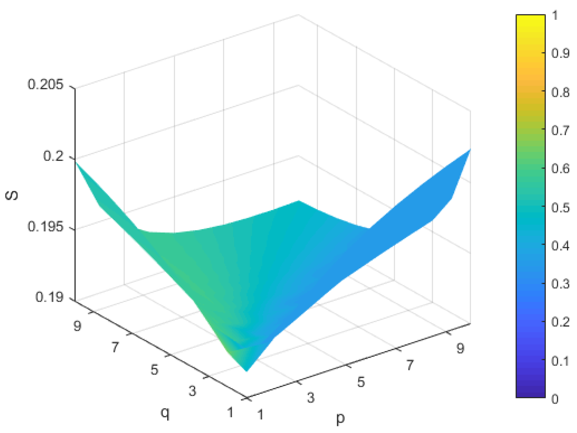
5.2. Sensitivity Analysis

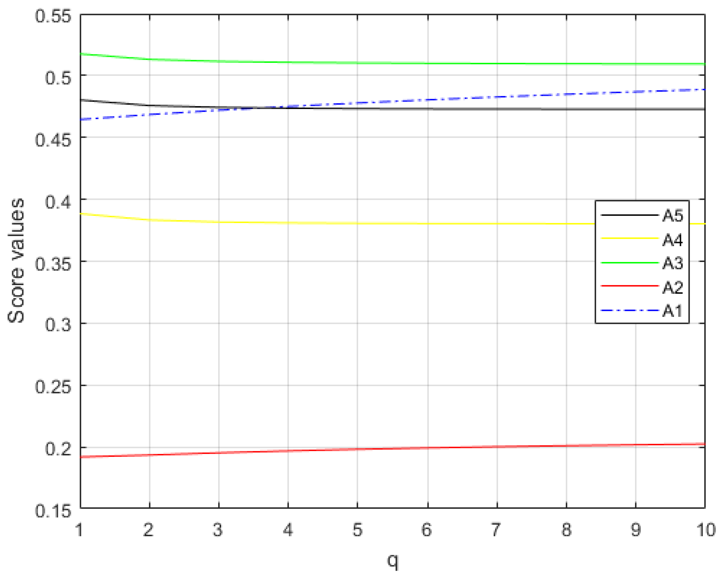
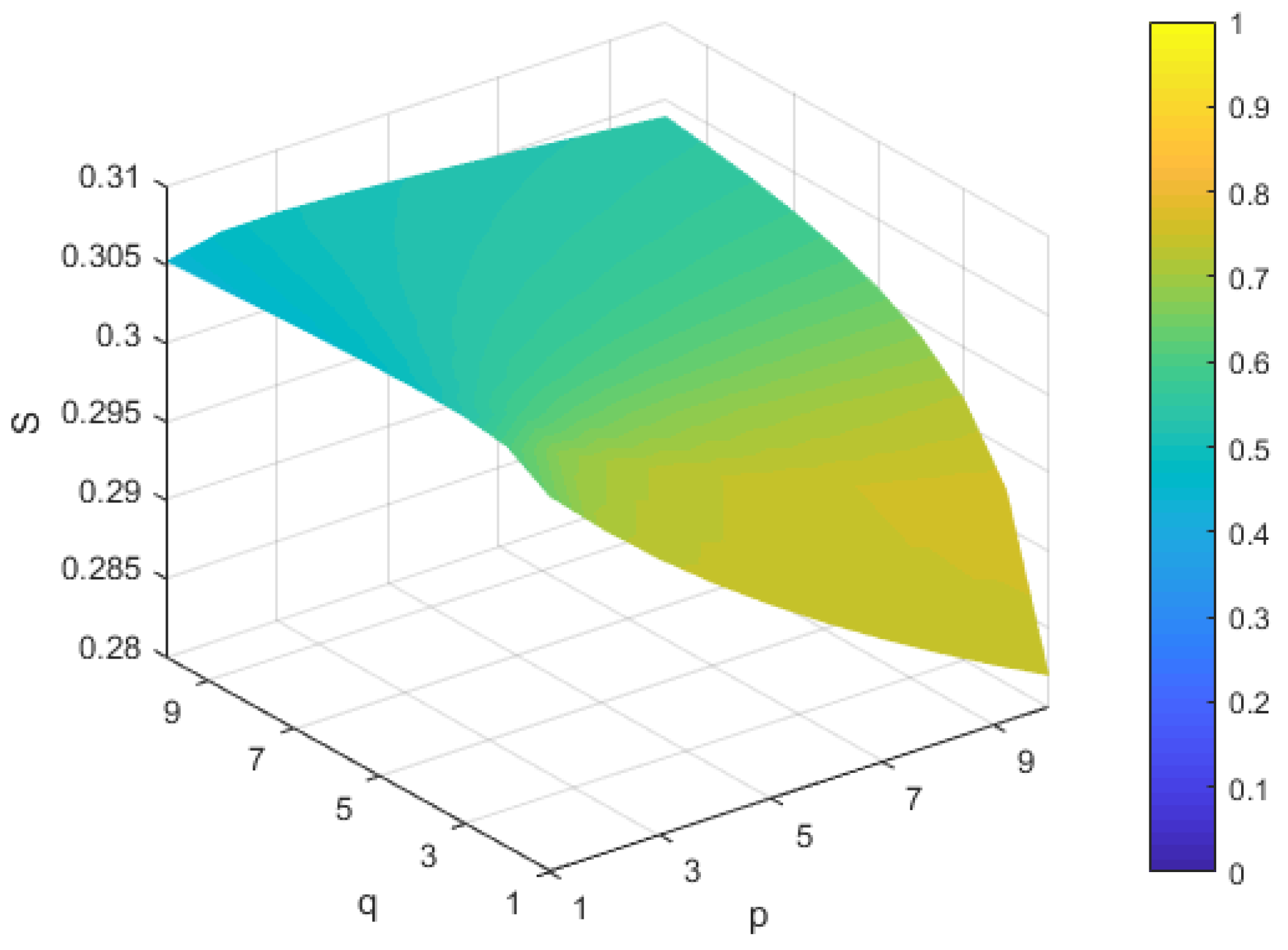
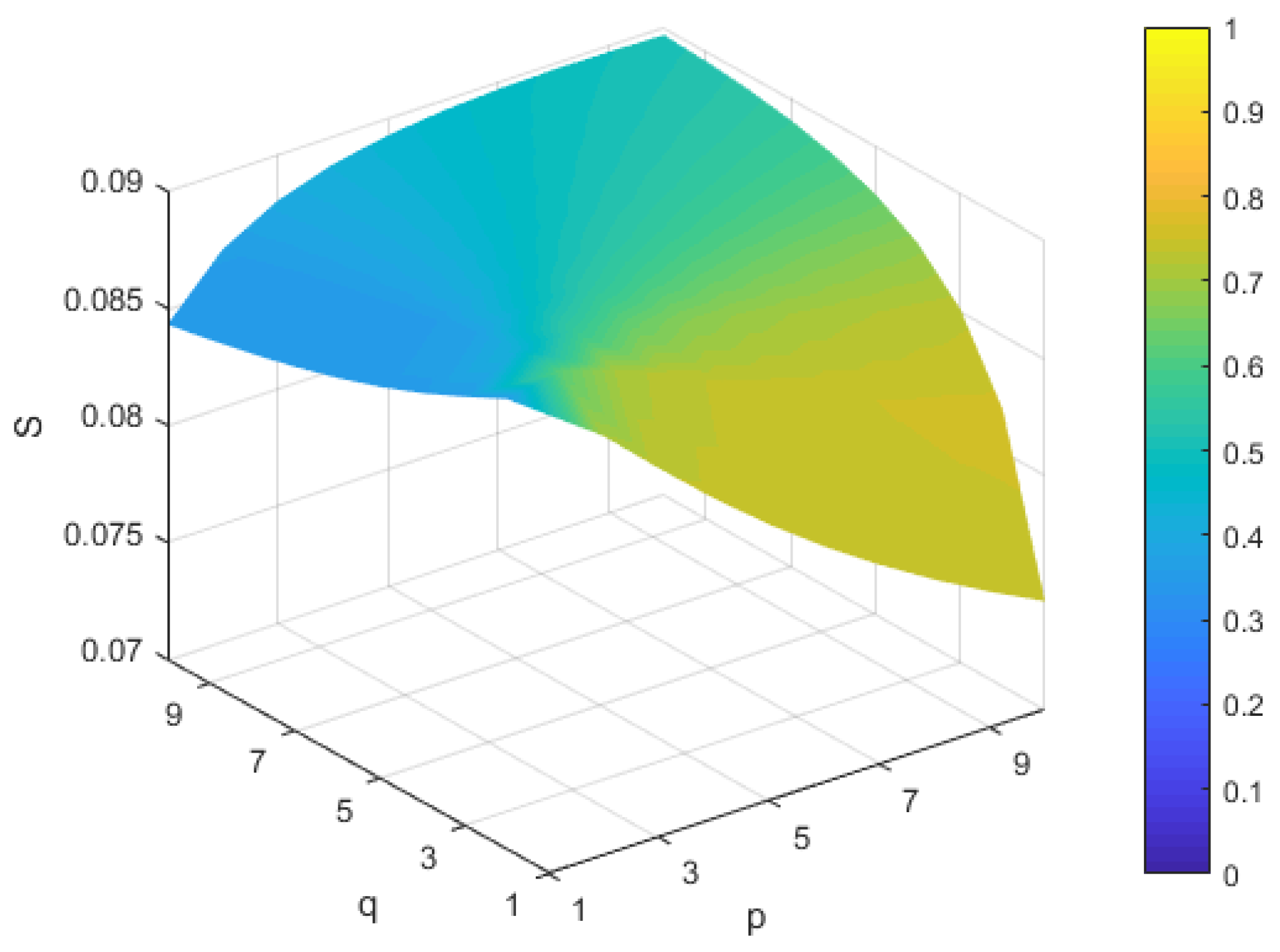
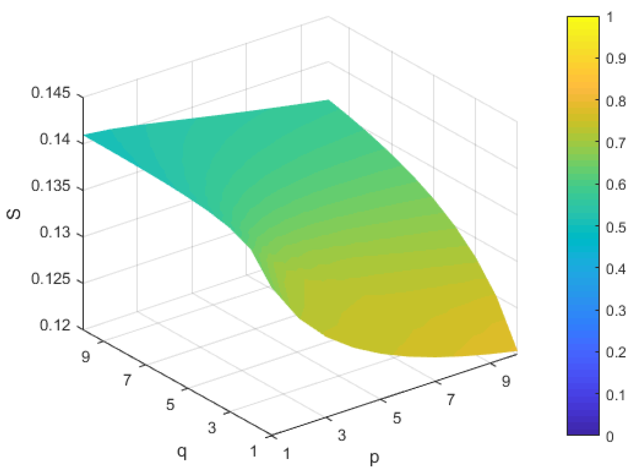
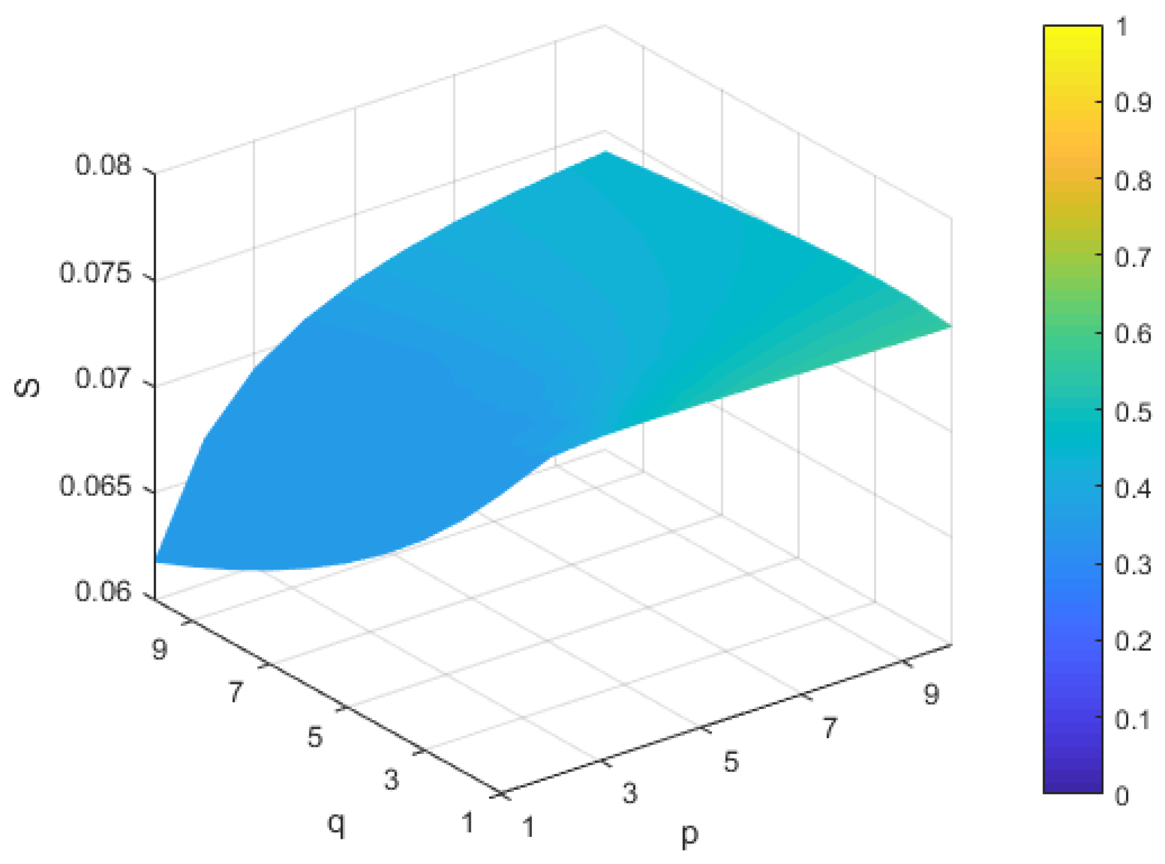
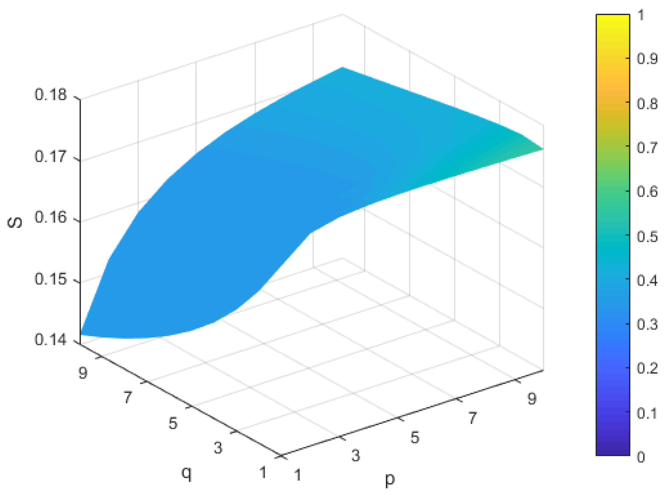
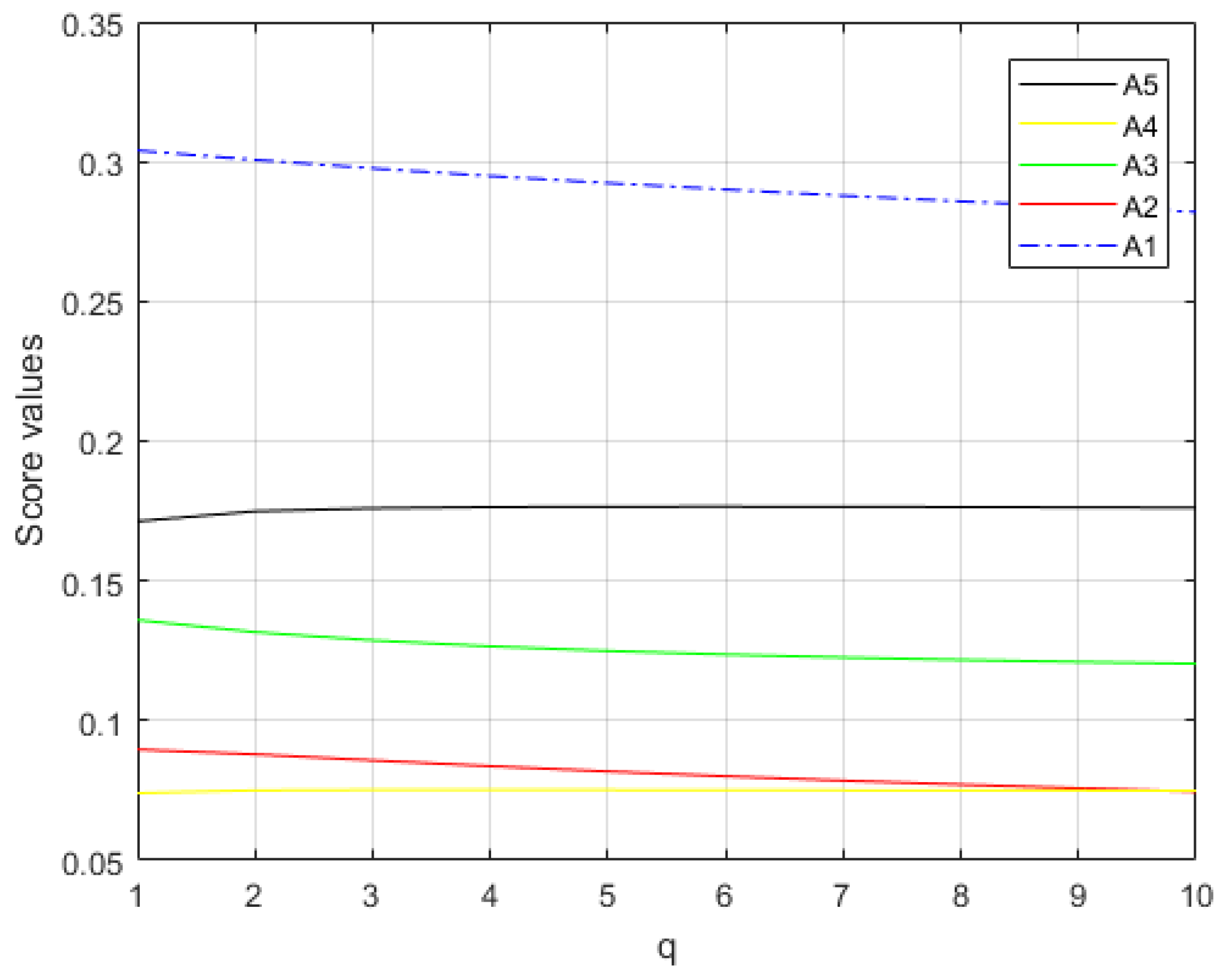
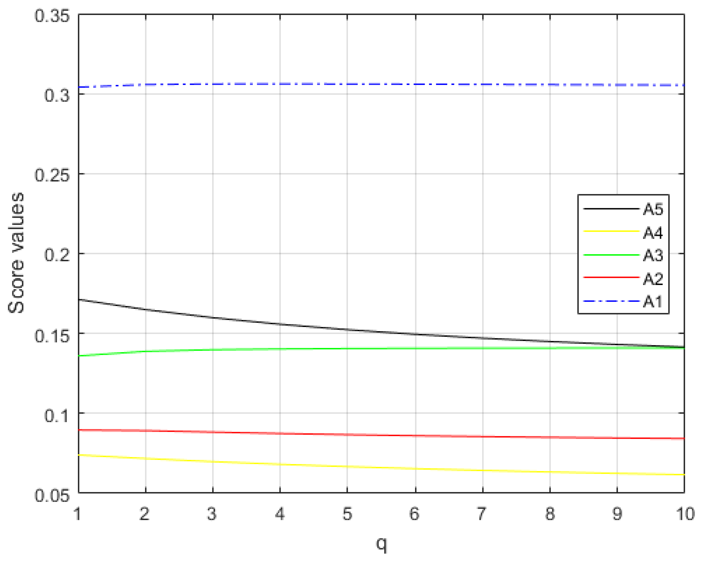
The flexibilities of the proposed method are reflected in two aspects. Firstly, it is based on DTT so that the information aggregation process is also flexible. Secondly, it is based on HM which has two important parameters, playing crucial role in the decision results. Hence, different scores of alternatives and ranking orders may be obtained with respect to the parameters p and q. In the following, we shall investigate the influence of the parameters on the results. Firstly, we assign different values to p and q and scores of alternatives are presented as Figure 2, Figure 3, Figure 4, Figure 5 and Figure 6. In addition, we let p (or q) be a fixed set, and we investigate the influence of q (or p) on the scores’ functions and ranking results. Details can be found in Figure 7 and Figure 8.

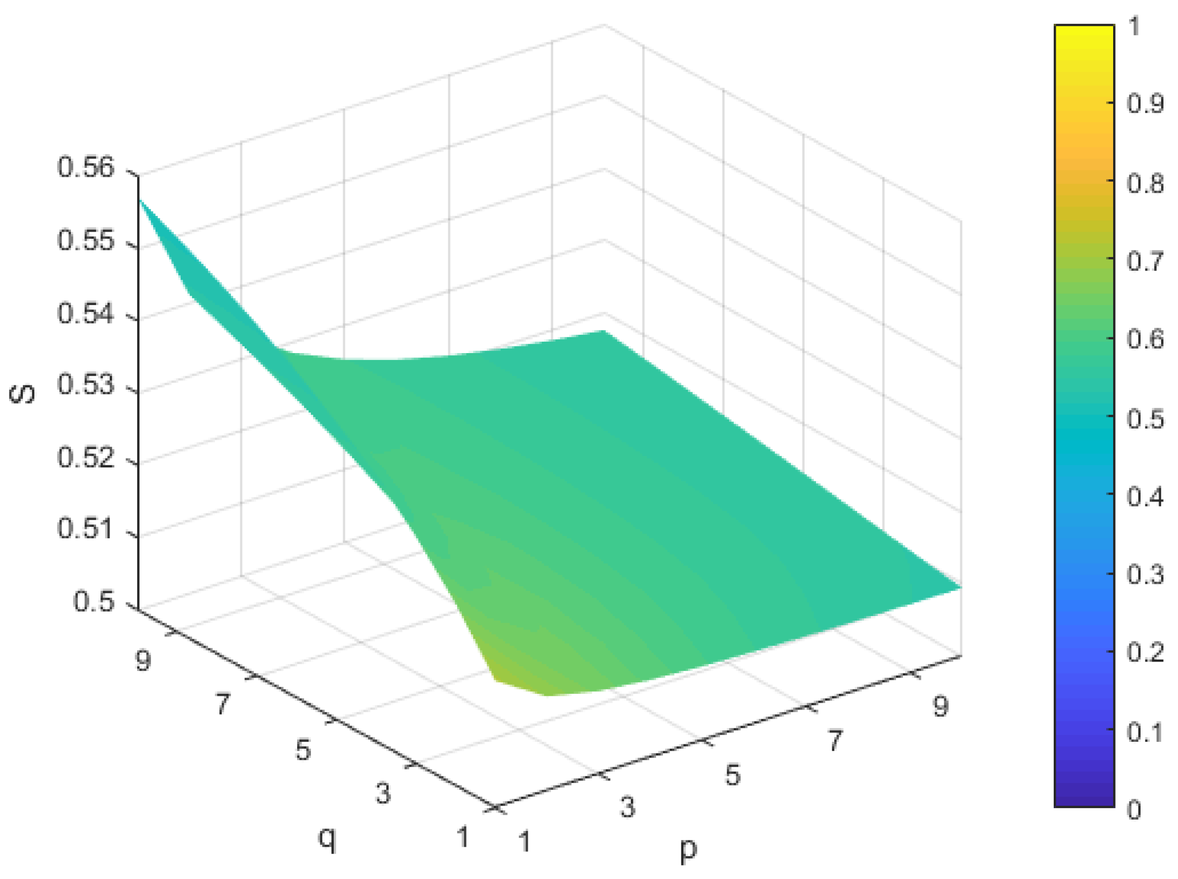
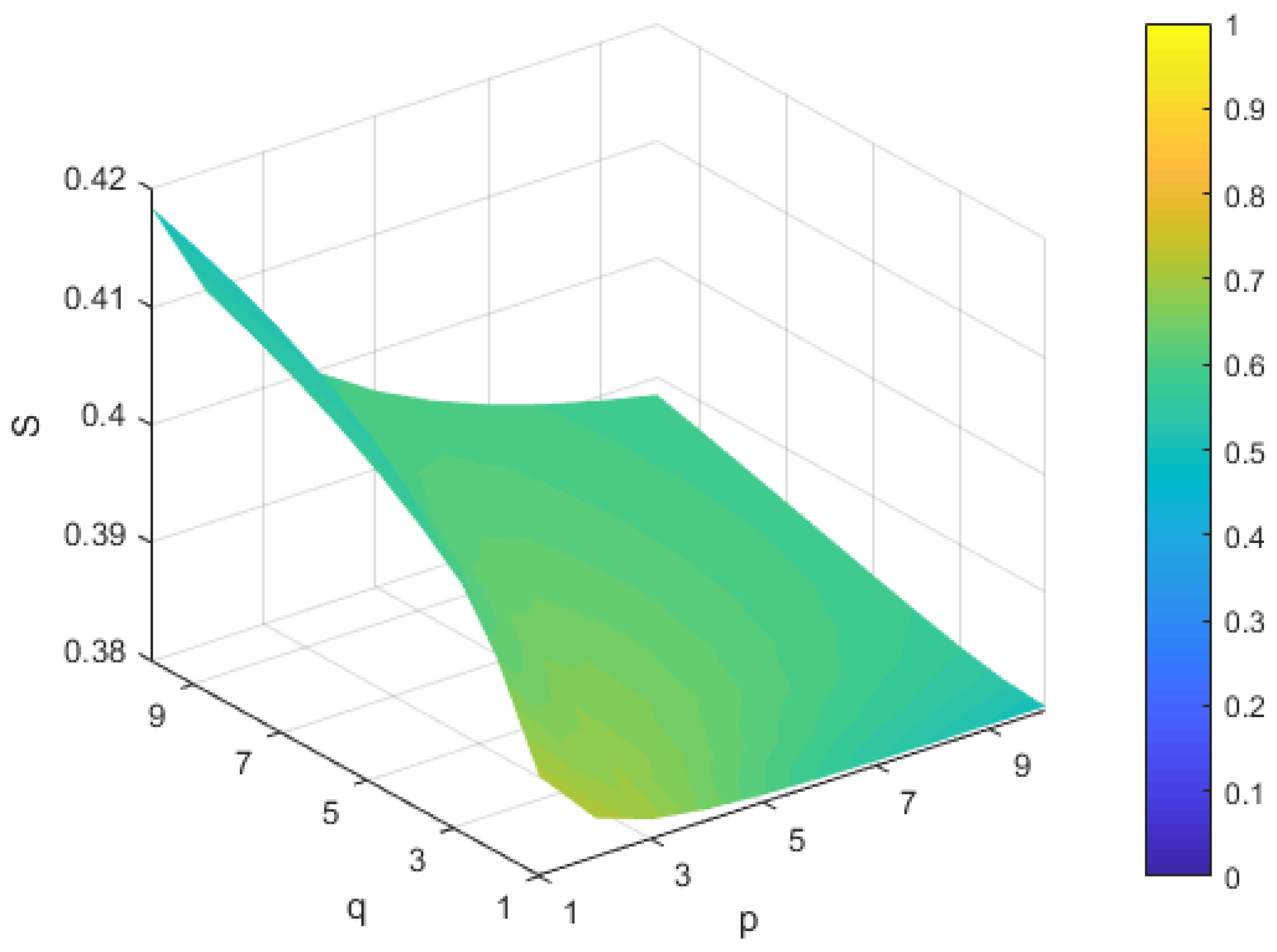
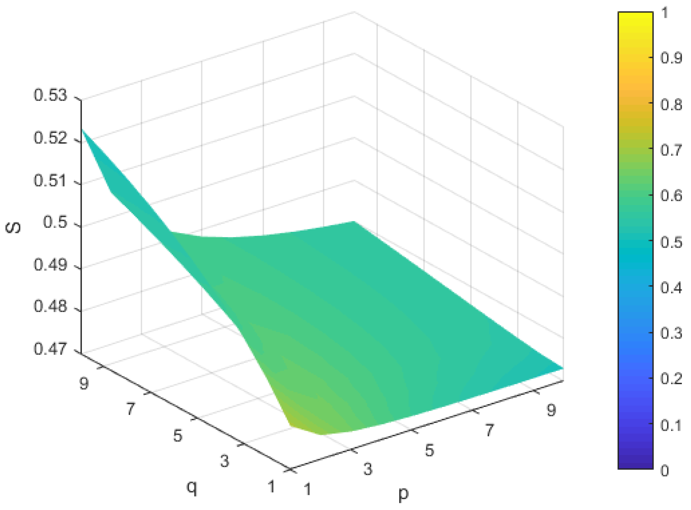
Form Figure 2, Figure 3, Figure 4, Figure 5 and Figure 6, we can find out that different scores of alternatives can be derived with respect to different parameters p and q. This characteristic illustrates the flexibility of the proposed method and operators. In real MADM problems, the values of p and q can be determined by decision-makers according to actual needs. In Figure 7 and Figure 8, we investigate the individual effect of the parameters p and q on the score function and ranking results, i.e., we let p or q be a fixed value and investigate the influence of another parameter on the ranking results. As we can see from the Figure 7 and Figure 8, different scores and ranking results can be obtained with the change of p or q. This characteristics also reflects the flexibility of the proposed PFDWHM operator as well as the corresponding MADM method. Additionally, it can be noticed that no matter what the values of p and q are, the best alternatives are always $A_3$, and the worst alternatives are always $A_2$. This feature demonstrates the robustness of the proposed method. It is worth pointing out that in the above discussion, we used the proposed PFDWHM operator to aggregate decision-makers’ preference information. In the following, we investigate the influence of parameters p and q on the scores and ranking orders in the PFDWGHM operators. Analogously, we assign the different values to the parameters p and q and the corresponding scores of alternatives and ranking orders are derived. Details can be found in Figure 9, Figure 10, Figure 11, Figure 12, Figure 13, Figure 14 and Figure 15.

In this section, we investigate the influence of the parameters on the scores and ranking orders. Results illustrate the flexibility and powerfulness of the proposed method. Moreover, the proposed method exhibit high robustness in the process of information aggregation and MADM. Thus, the proposed method is sufficient to deal with practical MADM problems.

5.3. Comparative Analysis

The main contribution of this paper is that we proposed a powerful MADM method with picture fuzzy information. In Section 5.1, we illustrated the performance of the proposed method by solving a real decision-making problem. In the following, we compare the newly proposed method with exiting picture fuzzy MADM methods. We utilize the method introduced by Wei [45] based on the picture fuzzy weighted average (PFWA) operator, the method put forward by Wei [49] based on the picture fuzzy Hamacher weighted average operator (PFHWA), and our method based on PFDWHM operator to solve the above example, and present the score function and ranking orders in

Table 2. Score function and ranking results by different results.

Method	$\mathbf{Score}\mathbf{Function}\mathbf{of}\mathit{S}\left({\mathit{\alpha }}_{\mathit{i}}\right)\left(\mathit{i}=1,2,3,4,5\right)$	Ranking Results
Wei’s [45] method based on picture fuzzy weighted average (PFWA) operator	$S\left({\alpha }_1\right)=0.3792$$S\left({\alpha }_2\right)=0.4526$$S\left({\alpha }_3\right)=0.5608$ $S\left({\alpha }_4\right)=0.3674$$S\left({\alpha }_5\right)=0.4114$	$A_3>A_2>A_5>A_1>A_4$
Wei’s [49] method based on picture fuzzy Hamacher weighted average operator (PFHWA) operator ($\lambda =2$)	$S\left({\alpha }_1\right)=0.3473$$S\left({\alpha }_2\right)=0.4119$$S\left({\alpha }_3\right)=0.5205$ $S\left({\alpha }_4\right)=0.3088$$S\left({\alpha }_5\right)=0.3528$	$A_3>A_2>A_5>A_1>A_4$
The proposed method based on PFDWHM operator $(\lambda =2,p,q=1$)	$S\left({\alpha }_1\right)=0.4645$$S\left({\alpha }_2\right)=0.1918$$S\left({\alpha }_3\right)=0.5176$ $S\left({\alpha }_4\right)=0.3885$$S\left({\alpha }_5\right)=0.4803$	$A_3>A_5>A_4>A_1>A_2$

.

From Table 2, it is easy to find out that the ranking result derived by Wei’s [45] method is different from that obtained by the proposed method. The reasons are two-fold. Firstly, Wei’s [49] method is based on simple algebraic operations, whereas the operational laws of our method are based on the DTT. Obviously, operations of PFNs based on DTT are more flexible than algebraic operations. Thus, our method makes the information aggregation process more flexible. Additionally, our method is based on the HM operator so that the interrelationship between attributes can be reflected. Wei’s [45] method is based on the simple weighted average operator and the interrelationship between attributes is ignored. Thus, our method is more powerful, flexible and suitable than that proposed by Wei [45] for dealing with MADM problems.

The method based on the PFHWA operator proposed by Wei [49] is based on Hamacher t-norm and t-conorm. Thus, it is more flexible than Wei’s [45] method based on the PFWA operator. However, Wei’s [49] method is based on the simple weighted average operator which is the same as that proposed by Wei [45]. Thus, Wei’s [49] method based on the PFHWA do not consider the interrelationships among attribute values either. Our method based on the PFDWHM has the capability of capturing the interrelationship between attributes. Thus, our method is more powerful than Wei’s [49] method.

To sum up, the novelties and powerfulness of the proposed method are two-fold. Firstly, our method is based on the DTT, which makes the information aggregation flexible as there is a parameter $\lambda$. Secondly, the proposed method is based on the PFDWHM operator so that the interrelationship between attributes is captured. This characteristic makes it more suitable for dealing with practical MADM problems. Thus, our method is more powerful and flexible than existing picture fuzzy MADM methods.

6. Conclusions

Recently, PFS has become more powerful than IFS as it takes decision-makers’ neutrality degree into consideration. This paper proposed some novel picture fuzzy aggregation operators based on DTT. Firstly, we introduced novel operational rules of PFNs on the basis of DTT. Then, we extended HM to PFSs based on the newly proposed picture fuzzy operations and proposed the PFDHM, PFDWHM, PFDGHM, and PFDWGHM operators. The proposed picture fuzzy aggregation operators not only capture the interrelationship among PFNs, but also make the information aggregation process more flexible. We further introduced a novel approach for MADM with picture fuzzy information. An ERP provider selection illustrated the validity of the proposed method. We also investigated influence of the parameters on the decision results in the newly developed picture fuzzy aggregation operators. We also compared the proposed method with others to demonstrate its superiorities and advantages In future work, we shall continue to investigate picture fuzzy aggregation operators, such as picture fuzzy Hamy mean operators and generalized picture fuzzy Hamy mean operators.

References

- Medina, J.; Ojeda-Aciego, M. Multi-adjoint t-concept lattices. Inf. Sci. 2010, 180, 712–725. [Google Scholar] [CrossRef]
- Pozna, C.; Minculete, N.; Precup, R.E.; Kóczy, L.T.; Ballagi, Á. Signatures: Definitions, operators and applications to fuzzy modelling. Fuzzy Sets Syst. 2012, 201, 86–104. [Google Scholar] [CrossRef]
- Jankowski, J.; Kazienko, P.; Wątróbski, J.; Lewandowska, A.; Ziemba, P.; Ziolo, M. Fuzzy multi-objective modeling of effectiveness and user experience in online advertising. Expert Syst. Appl. 2016, 65, 315–331. [Google Scholar] [CrossRef]
- Kumar, A.; Kumar, D.; Jarial, S.K. A hybrid clustering method based on improved artificial bee colony and fuzzy C-means algorithm. Int. J. Artif. Intell. 2017, 15, 40–60. [Google Scholar]
- Blanco-Mesa, F.; Gil-Lafuente, A.M.; Merigo, J.M. Fuzzy decision making: A bibliometric-based review. J. Intell. Fuzzy Syst. 2017, 32, 2033–2050. [Google Scholar] [CrossRef] [Green Version]
- Merigó, J.M.; Gil-Lafuente, A.M.; Yager, R.R. An overview of fuzzy research with bibliometric indicators. Appl. Soft Comput. 2015, 27, 420–433. [Google Scholar] [CrossRef]
- Shi, Z.J.; Wang, X.Q.; Palomares, I.; Guo, S.J.; Ding, R.X. A novel consensus model for multi-attribute large-scale group decision making based on comprehensive behavior classification and adaptive weight updating. Knowl.-Based Syst. 2018, 158, 196–208. [Google Scholar] [CrossRef]
- Xing, Y.P.; Zhang, R.T.; Wang, J.; Zhu, X.M. Some new Pythagorean fuzzy Choquet–Frank aggregation operators for multi-attribute decision making. Int. J. Fuzzy Syst. 2018, 33, 2189–2215. [Google Scholar] [CrossRef]
- Xu, Y.; Shang, X.P.; Wang, J.; Wu, W.; Huang, H.Q. Some q-rung dual hesitant fuzzy Heronian mean operators with their application to multiple attribute group decision-making. Symmetry 2018, 10, 472. [Google Scholar] [CrossRef]
- Mao, X.B.; Hu, S.S.; Dong, J.Y.; Wan, S.P.; Xu, G.L. Multi-attribute group decision making based on cloud aggregation operators under interval-valued hesitant fuzzy linguistic environment. Int. J. Fuzzy Syst. 2018, 20, 2273–2300. [Google Scholar] [CrossRef]
- Wang, J.; Zhang, R.T.; Zhu, X.M.; Xing, Y.P.; Buchmeister, B. Some hesitant fuzzy linguistic Muirhead means with their application to multiattribute group decision-making. Complexity 2018, 2018, 5087851. [Google Scholar] [CrossRef]
- Yu, G.F.; Li, D.F.; Fei, W. A novel method for heterogeneous multi-attribute group decision making with preference deviation. Comput. Ind. Eng. 2018, 124, 58–64. [Google Scholar] [CrossRef]
- Zhang, R.T.; Wang, J.; Zhu, X.M.; Xia, M.M.; Yu, M. Some generalized Pythagorean fuzzy Bonferroni mean aggregation operators with their application to multiattribute group decision-making. Complexity 2017, 2017, 5937376. [Google Scholar] [CrossRef]
- Li, L.; Zhang, R.T.; Wang, J.; Zhu, X.M.; Xing, Y.P. Pythagorean fuzzy power Muirhead mean operators with their application to multi-attribute decision making. J. Intell. Fuzzy Syst. 2018, 35, 2035–2050. [Google Scholar] [CrossRef]
- Li, L.; Zhang, R.T.; Wang, J.; Shang, X.P.; Bai, K.Y. A novel approach to multi-attribute group decision-making with q-rung picture linguistic information. Symmetry. 2018, 10, 172. [Google Scholar] [CrossRef]
- Zadeh, L.A. Fuzzy sets. Inf. Control 1965, 8, 338–353. [Google Scholar] [CrossRef] [Green Version]
- Atanassov, K.T. Intuitionistic fuzzy sets. Fuzzy Sets Syst. 1986, 20, 87–96. [Google Scholar] [CrossRef]
- Xu, Z.S. Intuitionistic fuzzy aggregation operators. IEEE Trans. Fuzzy Syst. 2007, 15, 1179–1187. [Google Scholar]
- Xu, Z.S.; Yager, R.R. Some geometric aggregation operators based on intuitionistic fuzzy sets. Int. J. Gen. Syst. 2006, 35, 417–433. [Google Scholar] [CrossRef]
- Wang, W.Z.; Liu, X.F. Intuitionistic fuzzy information aggregation using Einstein operations. IEEE Trans. Fuzzy Syst. 2012, 20, 923–938. [Google Scholar] [CrossRef]
- Zhang, Z.M. Multi-criteria group decision-making methods based on new intuitionistic fuzzy Einstein hybrid weighted aggregation operators. Neural Comput. Appl. 2017, 28, 3781–3800. [Google Scholar] [CrossRef]
- Xu, Z.S.; Yager, R.R. Intuitionistic fuzzy Bonferroni means. IEEE Trans. Syst. Man Cybern. B Cybern. 2011, 41, 568–578. [Google Scholar] [PubMed]
- Xia, M.M.; Xu, Z.S.; Zhu, B. Geometric Bonferroni means with their application in multi-criteria decision making. Knowl.-Based Syst. 2013, 40, 88–100. [Google Scholar] [CrossRef]
- Qin, J.D.; Liu, X.W. An approach to intuitionistic fuzzy multiple attribute decision making based on Maclaurin symmetric mean operators. J. Intell. Fuzzy Syst. 2014, 27, 2177–2190. [Google Scholar]
- Yu, D.J. Intuitionistic fuzzy geometric Heronian mean aggregation operators. Appl. Soft Comput. 2013, 13, 1235–1246. [Google Scholar] [CrossRef]
- Liu, P.D.; Li, D.F. Some Muirhead mean operators for intuitionistic fuzzy numbers and their applications to group decision making. PLoS ONE 2017, 12, e0168767. [Google Scholar] [CrossRef] [PubMed]
- Ren, H.P.; Chen, H.H.; Fei, W.; Li, D.F. A MAGDM method considering the amount and reliability information of interval-valued intuitionistic fuzzy sets. Int. J. Fuzzy Syst. 2017, 19, 715–725. [Google Scholar] [CrossRef]
- Afful-Dadzie, E.; Oplatkova, Z.K.; Prieto, L.A.B. Comparative state-of-the-art survey of classical fuzzy set and intuitionistic fuzzy sets in multi-criteria decision making. Int. J. Fuzzy Syst. 2017, 19, 726–738. [Google Scholar] [CrossRef]
- Tao, Z.F.; Liu, X.; Chen, H.Y.; Zhou, L.G. Ranking interval-valued fuzzy numbers with intuitionistic fuzzy possibility degree and its application to fuzzy multi-attribute decision making. Int. J. Fuzzy Syst. 2017, 19, 646–658. [Google Scholar] [CrossRef]
- Peng, J.J.; Wang, J.Q.; Wu, X.H.; Tian, C. Hesitant intuitionistic fuzzy aggregation operators based on the Archimedean t-norms and t-conorms. Int. J. Fuzzy Syst. 2017, 19, 702–714. [Google Scholar] [CrossRef]
- Yuan, J.H.; Li, C.B. A new method for multi-attribute decision making with intuitionistic trapezoidal fuzzy random variable. Int. J. Fuzzy Syst. 2017, 19, 5–26. [Google Scholar] [CrossRef]
- Zhang, Z.M. Several new interval-valued intuitionistic fuzzy Hamacher hybrid operators and their application to multi-criteria group decision making. Int. J. Fuzzy Syst. 2016, 18, 829–848. [Google Scholar] [CrossRef]
- He, Y.D.; He, Z.; Shi, L.X. Multiple attributes decision making based on scaled prioritized intuitionistic fuzzy interaction aggregation operators. Int. J. Fuzzy Syst. 2016, 18, 924–938. [Google Scholar] [CrossRef]
- Wei, G. Approaches to interval intuitionistic trapezoidal fuzzy multiple attribute decision making with incomplete weight information. Int. J. Fuzzy Syst. 2015, 17, 484–489. [Google Scholar] [CrossRef]
- Cuong, B. Picture fuzzy sets-first results. Part 1. Semin. Neuro Fuzzy Syst Appl. 2013. [CrossRef]
- Le, H.S.; Viet, P.V.; Hai, P.V. Picture inference system: A new fuzzy inference system on picture fuzzy set. Appl. Intell. 2017, 46, 652–669. [Google Scholar]
- Son, L.H. Generalized picture distance measure and applications to picture fuzzy clustering. Appl. Soft Comput. 2016, 46, 284–295. [Google Scholar] [CrossRef]
- Yang, Y.; Liang, C.C.; Ji, S.W.; Liu, T. Adjustable soft discernibility matrix based on picture fuzzy soft sets and its applications in decision making. J. Intell. Fuzzy Syst. 2015, 29, 1711–1722. [Google Scholar] [CrossRef]
- Wei, G.W. Picture fuzzy cross-entropy for multiple attribute decision making problems. J. Bus. Econ. Manag. 2016, 17, 491–502. [Google Scholar] [CrossRef]
- Bo, C.; Zhang, X. New operations of picture fuzzy relations and fuzzy comprehensive evaluation. Symmetry 2017, 9, 268. [Google Scholar] [CrossRef]
- Peng, X.D.; Dai, J.G. Algorithm for picture fuzzy multiple attribute decision-making based on new distance measure. Int. J. Uncertain. Quantif. 2017, 7, 2. [Google Scholar] [CrossRef]
- Wei, G.W.; Alsaadi, F.E.; Hayat, T.; Alsaedi, A. Picture 2-tuple linguistic aggregation operators in multiple attribute decision making. Soft Comput. 2018, 22, 989–1002. [Google Scholar] [CrossRef]
- Wei, G.W. Picture 2-tuple linguistic Bonferroni mean operators and their application to multiple attribute decision making. Int. J. Fuzzy Syst. 2017, 19, 997–1010. [Google Scholar] [CrossRef]
- Wei, G.W. Some cosine similarity measures for picture fuzzy sets and their applications to strategic decision making. Informatica 2017, 28, 547–564. [Google Scholar] [CrossRef]
- Wei, G.W. Picture fuzzy aggregation operators and their application to multiple attribute decision making. J. Intell. Fuzzy Syst. 2017, 33, 713–724. [Google Scholar] [CrossRef]
- Garg, H. Some picture fuzzy aggregation operators and their applications to multicriteria decision-making. Arab. J. Sci. Eng. 2017, 42, 5275–5290. [Google Scholar] [CrossRef]
- Li, D.X.; Dong, H.; Jin, X. Model for evaluating the enterprise marketing capability with picture fuzzy information. J. Intell. Fuzzy Syst. 2017, 33, 3255–3263. [Google Scholar] [CrossRef]
- Peng, S.M. Study on enterprise risk management assessment based on picture fuzzy multiple attribute decision-making method. J. Intell. Fuzzy Syst. 2017, 33, 3451–3458. [Google Scholar] [CrossRef]
- Wei, G.W. Picture fuzzy Hamacher aggregation operators and their application to multiple attribute decision making. Fund. Inform. 2018, 157, 271–320. [Google Scholar] [CrossRef]
- Dombi, J. A general class of fuzzy operators, the De-Morgan class of fuzzy operators and fuzziness induced by fuzzy operators. Fuzzy Sets Syst. 1982, 8, 149–163. [Google Scholar] [CrossRef]
- Liu, P.D.; Liu, J.L.; Chen, S.M. Some intuitionistic fuzzy Dombi Bonferroni mean operators and their application to multi-attribute group decision making. J. Oper. Res. Soc. 2018, 69, 1–24. [Google Scholar] [CrossRef]
- He, X.R. Typhoon disaster assessment based on Dombi hesitant fuzzy information aggregation operators. Nat. Hazards 2018, 90, 1153–1175. [Google Scholar] [CrossRef]
- Chen, J.Q.; Ye, J. Some single-valued neutrosophic Dombi weighted aggregation operators for multiple attribute decision-making. Symmetry 2017, 9, 82. [Google Scholar] [CrossRef]
- Bonferroni, C. Sulle medie multiple di potenze. Boll. Unione Mat. Ital. 1950, 5, 267–270. [Google Scholar]
- Sykora, S. Mathematical means and averages: Generalized Heronian means. Stans Lib. 2009. [Google Scholar] [CrossRef]
- Yu, D.J.; Wu, Y.Y. Interval-valued intuitionistic fuzzy Heronian mean operators and their application in multi-criteria decision making. Afr. J. Bus. Manag. 2012, 6, 4158–4168. [Google Scholar] [CrossRef]
Figure 1.
The algorithm flow of picture MADM problems.
Figure 2.
Score of A1 when based on the picture fuzzy Dombi weighted Heronian mean (PFDWHM) operator (λ = 2).
Figure 3.
Score of A2 when based on the PFDWHM operator (λ = 2).
Figure 4.
Score of A3 when based on the PFDWHM operator (λ = 2).
Figure 5.
Score of A4 when based on the PFDWHM operator (λ = 2).
Figure 6.
Score of A5 when based on the PFDWHM operator (λ = 2).
Figure 7.
Scores of alternative Ai (i = 1, 2, 3, 4, 5) when p = 1 and based on the PFDWHM operator (λ = 2).
Figure 8.
Scores of alternative Ai (i = 1, 2, 3, 4, 5) when q = 1 and based on the PFDWHM operator (λ = 2).
Figure 9.
Score of A1 when based on the picture fuzzy Dombi weighted geometric Heronian mean (PFDWGHM) operator (λ = 2).
Figure 10.
Score of A2 when based on the PFDWGHM operator (λ = 2).
Figure 11.
Score of A3 when based on the PFDWGHM operator (λ = 2).
Figure 12.
Score of A4 when based on the PFDWGHM operator (λ = 2).
Figure 13.
Score of A5 when based on the PFDWGHM operator (λ = 2).
Figure 14.
Scores of alternative Ai (i = 1, 2, 3, 4, 5) when p = 1 and based on the PFDWGHM operator (λ = 2).
Figure 15.
Scores of alternative Ai (i = 1, 2, 3, 4, 5) when q = 1 and based on the PFDWGHM operator (λ = 2).