
Optimal Design of the Proton-Exchange Membrane Fuel Cell Connected to the Network Utilizing an Improved Version of the Metaheuristic Algorithm
1
College of Public Administration and Emergency Management, Jinan University, Guangzhou 510632, China
2
School of Marxism, Hunan City University, Yiyang 413000, China
3
Young Researchers and Elite Club, Ardabil Branch, Islamic Azad University, Ardabil 5615731567, Iran
*
Authors to whom correspondence should be addressed.
Sustainability 2023, 15(18), 13877; https://doi.org/10.3390/su151813877
Submission received: 19 May 2023
/
Revised: 27 August 2023
/
Accepted: 30 August 2023
/
Published: 18 September 2023
(This article belongs to the Special Issue Renewable Energy Generation and Management Systems for Sustainable Development)
Abstract
:Fuel cells are a newly developed source for generating electric energy. These cells produce electricity through a chemical reaction between oxygen and hydrogen, which releases electrons. In recent years, extensive research has been conducted in this field, leading to the emergence of high-power batteries. This study introduces a novel technique to enhance the power quality of grid-connected proton-exchange membrane (PEM) fuel cells. The proposed approach uses an inverter following a buck converter that reduces voltage. A modified pelican optimization (MPO) algorithm optimizes the controller firing. A comparison is made between the controller’s performance, based on the recommended MPO algorithm and various other recent approaches, demonstrating the superior efficiency of the MPO algorithm. The study’s findings indicate that the current–voltage relationship in proton-exchange membrane fuel cells (PEMFCs) follows a logarithmic pattern, but becomes linear in the presence of ohmic overvoltage. Furthermore, the PEMFC operates at an impressive efficiency of 60.43% when running at 8 A, and it can deliver a significant power output under specific operating conditions. The MPO algorithm surpasses other strategies in terms of efficiency and reduction in voltage deviation, highlighting its effectiveness in managing the voltage stability, and improving the overall performance. Even during a 0.2 sagging event, the MPO-based controller successfully maintains the fuel cell voltage near its rated value, showcasing the robustness of the optimized regulators. The suggested MPO algorithm also achieves a superior accuracy in maintaining the voltage stability across various operating conditions.
1. Introduction
1.1. Background
Increasingly, the growth in the energy demand, pollution caused by burning fossil fuels, and the depletion of these fuel sources have resulted in extensive research on new energy conversion technologies [1]. Among these, two central policies have always been considered: the optimization of the existing energy system to increase efficiency and reduce energy consumption in these systems, and the utilization of novel technologies and renewable energy resources [2]. However, the uneconomical nature of these resources has led to a lack of widespread use of new energy sources compared with conventional fuels [3]. Fuel cells (FCs) comprise one of the technologies for converting energy from fossil fuels to electricity, with water and heat produced as by-products [4]. These technologies have been proposed as a means of producing clean energy to replace conventional methods [5]. The main attraction of these cells is the production of useful and clean energy on a small scale, up to several hundred kilowatts [6]. The fuel cell system, as a whole, has an electrical efficiency between 40% and 60%, which is almost higher than many energy conversion systems [7]. FCs have various forms. These classifications have been defined according to the type of oxidizer and electrolyte, and the shovel temperature.
In the investigation of various types of FCs, PEMFCs (proton-exchange membrane fuel cells) include more specific benefits, which have led them to be compared with other fuel cells for dispersed production [8]. These advantages include a low start-up temperature, simple design, short start-up time, and high current density. Today, PEMFCs are widely developed in electrical appliances, naval vessels, spacecraft, a large variety of lightweight utilizations, hybrid power, and heat systems. Each proton-exchange membrane FC has three major parts: the electrolyte, anode, and cathode [9]. These parts are usually connected via bipolar plates. The polymer electrolyte only allows protons to pass through, and these protons go to the negative electrode. Through an exterior circuit, the electrons can move toward the cathode. Subsequently, an electric current is created via moving electrons through the external course [10]. The optimal design and development of the PEMFC will improve the output effectiveness through consideration of the reasons above, and it can minimize the total price. A set of partial or ordinary differential mathematical expressions that explain its features are involved in the modeling of the PEMFCs. The modeling of the PEMFCs will typically provide various significant benefits [11,12]. For example, mathematically, the PEM fuel cell model will help lead to a better model. Recent studies on the use of green energies (GEs) in electric vehicles (EVs) and electric grids have taken various forms. Researchers are motivated by this to offer improvements on energy-controlling policies within various energy sources, such as FCs.
1.2. Literature Review
The following arguments could be found via the field research that has been undertaken. Kanouni et al. [13] developed a multi-objective approach for a nonlinear model predictive regulator in a two-stage PEMFC converter linked to a double-phase grid. The version uses a multi-objective cost function to control the DC-link voltage balance and inverter currents, and to decrease the quantity of switch states. MATLAB/Simulink was used for the modeling of the performance of the inverter. The proposed process injects current into the network with a 2% THD, and provides MPP tracking.
Sun et al. [14] studied a grid-connected proton-exchange membrane FC in distributed production (DP), and found promising results. The current research mainly relies on the constant current (CC) mode, but new issues arise due to couplings generated via the CP procedure. Efficiency analysis shows static benchmarks for the oxygen excess ratio (OER), which conflicts with the voltage requirement of the inverter. Under CP mode, an unusual initial inverse response is observed in the dynamic operation, requiring a more cautious controller design. The simulation shows the feasibility and competence of the suggested strategy in correcting renewable intermittency, laying the groundwork for future grid-connected PEMFC research.
Liu et al. [15] proposed a solution-space-reduced model predictive control (MPC) for managing direct current (DC) and alternating current (AC) energy quality in two single-step-phase grid-connected PEM fuel cells, with a small DC-link capacitor capacitance. The article introduces a direct current control technique using a DC-link voltage notch filer, followed by a better MPC (model predictive control). The results validate the correctness and effectiveness of the suggested approach.
Zhang et al. [16] suggested an updated optimization technique for the optimal management of a grid-connected 1200 W PEM fuel cell. The Amended Penguin optimizer (APO) was employed to optimize the firing controller, achieving an optimum value of 53% at 7 A, and a maximum of 1200 W at 26 A and 46 V.
Reddy et al. [17] suggested a control technique on the basis of RBFN for grid-linked PEM fuel cell systems, with a large three-step-up IBC phase. For the grid-linked proton-exchange membrane FC, an MPPT (maximum power point tracking) controller on the basis of a neural network is presented. Interleaving delivers great power capabilities while reducing the voltage pressure on energy semi-conductor devices. It is suggested that the max power point tracking RBFN controller’s performance should be evaluated using the MATLAB 2018 or Simulink platform.
1.3. Contribution of the Study
In the present study, a new hybrid renewable system is employed, using the above clarifications to improve the system’s performance compared to other ones. While this technology boosts the electricity-producing efficiency, it degrades the power quality during distribution. We used a modified pelican optimization algorithm to resolve this problem, and to enhance this method. According to the findings, this strategy lessens the loss of the system’s power, harmony, and swelling.
The proposed technique of utilizing a modified model of the metaheuristic algorithm to optimize the design of a PEM fuel cell connected to the network has several justifications, including power quality enhancement through a reduction in the voltage and optimization of the firing controller through employing an inverter following a buck converter. It contributes to better power management, and overall power quality improvement. The modified pelican optimization (MPO) algorithm is chosen as the optimization technique for the controller design due to its superior efficiency compared to other recent approaches in various domains, as it can effectively optimize the control parameters for improved performance, by searching for optimal solutions in a vast solution space. The proposed technique is compared with various recent approaches, to demonstrate its superiority, highlighting the efficiency and effectiveness of the MPO algorithm in managing the voltage stability, and improving the overall performance, thereby justifying its selection over other alternatives. The findings of this study reveal that the current–voltage relationship in the PEMFC follows a logarithmic pattern, but becomes linear in the presence of ohmic overvoltage, allowing for the design of an optimized control strategy that considers the specific characteristics of the PEMFC, and ensures its efficient operation under different conditions. The study also demonstrates the impressive efficiency of the PEMFC, along with its capability to deliver a significant power output under specific operating conditions, emphasizing the importance of optimizing its design and control for enhanced performance as a high-power battery. The MPO-based controller exhibits robustness by successfully maintaining the fuel cell voltage near its rated value, indicating the effectiveness of the optimized regulators in voltage stability management. Furthermore, the suggested MPO algorithm achieves a superior accuracy in maintaining the voltage stability across various operating conditions, supporting its suitability for the proposed technique. The main contributions of the current research are thoroughly explained as the following:
- An enhanced grid-connected power quality in PEM fuel cells through the proposed technique;
- The utilization of a modified model of the metaheuristic algorithm, the modified pelican optimization (MPO) algorithm for the optimization of the controller design;
- The demonstration of the superiority of the proposed technique over other recent approaches, through a comparison study;
- Understanding the current–voltage relationship in PEMFCs, and its implications for designing an optimized control strategy;
- An impressive efficiency (60.43%) and significant output power in the PEMFC under specific operating conditions;
- The robustness of the MPO-based controller in maintaining the fuel cell voltage near its rated value, even during sagging events;
- The superior accuracy of the MPO algorithm in maintaining the voltage stability across various operating conditions.
2. System Modeling
2.1. The Main Structure
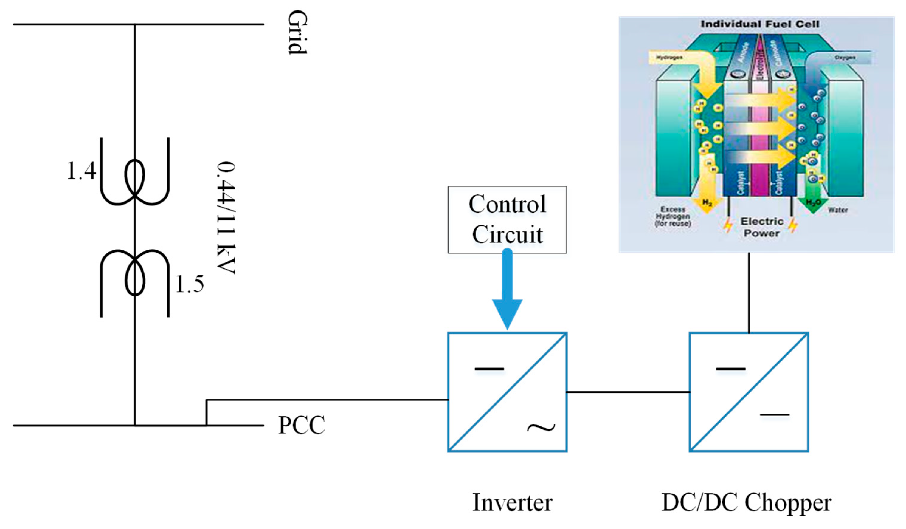
The schema of the system under investigation is represented in Figure 1. In the current research, a PEMFC-based system of renewable sources wired into the grid is employed as the best structure for managing electricity. A grid with a three-phase voltage resource is coupled to a parallel configuration of eight different 50 kW PEMFC systems. The output voltage of the fuel cell is 700 V; however, it is coupled to a buck converter, which lessens the produced voltage to 400 V. For the utilization of this direct current voltage, an inverter has been used.
For a customer to be able to use an AC voltage, an inverter is attached to the converter’s output. Last, but not least, a transformer is used to increase the amount of the voltage from 440 to 11,000 V, only to link the production of the FC to the electricity network at the point of common coupling (PCC). An optimal proportional integrator (PI) has been developed, to produce an effective result for the inverter. To achieve an effective on-grid FC for considering the excellent efficiency of the produced voltage at the PCC under various operational circumstances, this study seeks to use an optimal controller.
Table 1 indicates the system’s specification.
As can be observed from Table 1, each component (grid source, transformer, fuel cell converter, buck converter, and inverter) is listed with its respective parameters and corresponding example values. It provides a more obvious representation of the system specification. It is noteworthy that these values are only the case in some instances. They should be adapted in accordance with the unique requirements of the system.
2.2. Model of the PEMFC
Several models have been developed for PEMFC modeling. Larminie’s model [18] has been used in this essay. Gas pipelines continually deliver fuel to the cathode and anode sides. Firstly, the hydrogen is kept in air-oxidizing conditions, then pressurized storage tanks. Before entering the fuel cell, the air and hydrogen are moisturized. The diffusion layer of anode gas formed from paper carbon distributes hydrogen to the anode catalyst. is transformed into two electrons and two hydrogen ions in the catalyst particles [1].
The protons of created by the membrane go to the cathode’s catalyst layer. The electrons generated in the anode pass across the outside circular path, and do meaningful work prior to completing the chemical reaction on the grounds that the membrane is no longer conducting electrons. On the other part, is transferred over the diffusion layer of cathode gas; morevoer, water is formed, due to the reaction of protons and electrons at the surface of the CL (catalyst layer) [1]:
Therefore, the total reaction can be achieved as follows [1]:
The resulting voltage being reduced informs us that the irreversibility and entropy drops in a proton-exchange membrane FC are considered [19]. The high quantity of PEMFCs has to be linked hierarchically to generate the desired voltage, because the PEMFC system has a low voltage. Lastly, the polarization curve of the current voltage has a downward trend, due to the fact that the activation voltage of the proton-exchange membrane FC decreases, and the low-speed curve falls because of the ohmic-resistive voltage.
The output voltage of the PEMFC model can be obtained via the following equation [2]:
where describes the reversable potential, and and represent the ohmic and activation voltage losses, respectively.
The Nernst equation may be used to define the reversible voltage, which is the ideal maximum output voltage of the fuel cell. This value is determined according to the laws of thermodynamics.
where specifies the temperature in kelvin (K), the term describes the universal gas constant (8.314 J mol−1 K−1), determines the pressure in bars, and signifies the Faraday constant (96,485 C mol−1).
The resistance of ions or electrons in the various parts of the cell is what causes ohmic loss, which may be computed as follows:
where describes the anode catalyst layer, is the thickness, describes the conductivity, describes the mass flow rate, and signifies the effective value [5]. The superscripts and subscripts used in this context are as follows: BP, GDL, MPL, CL are the bipolar plate, gas diffusion layer, micro-porous layer, and catalyst layer, respectively.
In the above equation, the reaction rate is represented by j (A m−3), while the charge transfer coefficient is denoted by the symbol α, and the molar concentration of gas components is denoted by c (mol m−3). The superscripts and subscripts used in this context are as follows: stands for the reference, and represent, in turn, the anode and cathode, and and represent the anode and cathode catalyst layers. The heat and mass transfer equations, along with the parameters of the simulated PEMFC, can be achieved via [3].
2.3. Model of DC/DC Buck Converter
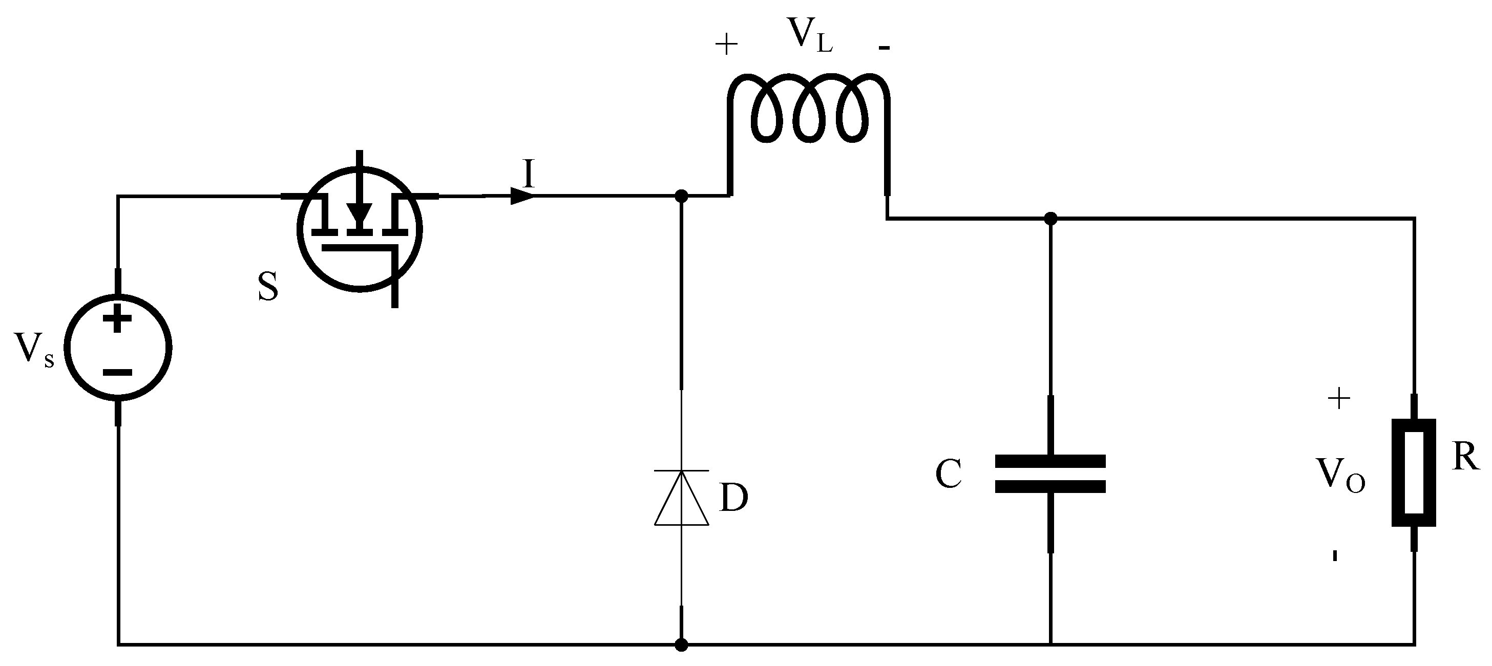
DC sources are used in many industrial applications, so a device is needed that is capable of converting a direct current voltage resource into a variable DC voltage resource. It is performed by a chopper [6]. A chopper is a DC-to-DC converter, which is like an AC transformer that can create the desired voltage by changing the number of turns, and it can directly convert the DC voltage to the wanted one continuously. A buck converter is the best device to reduce the output voltage. The structure of a buck converter is illustrated in Figure 2.
Regarding Figure 1, the voltage resource is linked to a solid-state semiconductor component or programmable power electronic component that operates as a switch, as seen in the picture above. This component might be a power MOSFET or an IGBT. Thyristors are no longer utilized in DC/DC converters, as shutting off a thyristor in the DC/DC circuit requires additional commutation, so another thyristor is required. Meanwhile, the power MOSFET could be turned off via the voltage supply for the resource bases and gate, and the IGBT may stop the operation via supplying voltage to the collector bases and gate.
A diode is another semiconductor switch utilized in the buck converter circuit. A circuit that is a filter that lets DC and signals of low-frequency go, and ceases signals that are high-frequency (a low-pass LC filter) is attached to the diode and switch. The filter is intended to minimize the voltage and current ripple. Figure 1 depicts a pure resistive load, as well. The circuit’s input voltage and the current traveling through the load are both constant. The load can also be regarded as a source of current.
Using wide-pulse modulation, a controlled switch is turned on and off (PWM). PWM can be based on frequency or time [5]. The downsides of frequency-based modulation include the need for a wide range of frequencies to ensure effective control and the desired output voltage. Because of the large frequency range, the low-pass LC filter requires a sophisticated design. In DC/DC converters, time-based modulation is commonly utilized. This modulation is simple to create and use, and the frequency remains constant. The current deviation in the buck converter and the produced voltage can be obtained based on the following equations.
where , , , and represent the capacitor, the inductance, the system current, and the produced voltage, respectively.
2.4. Model of Inverter
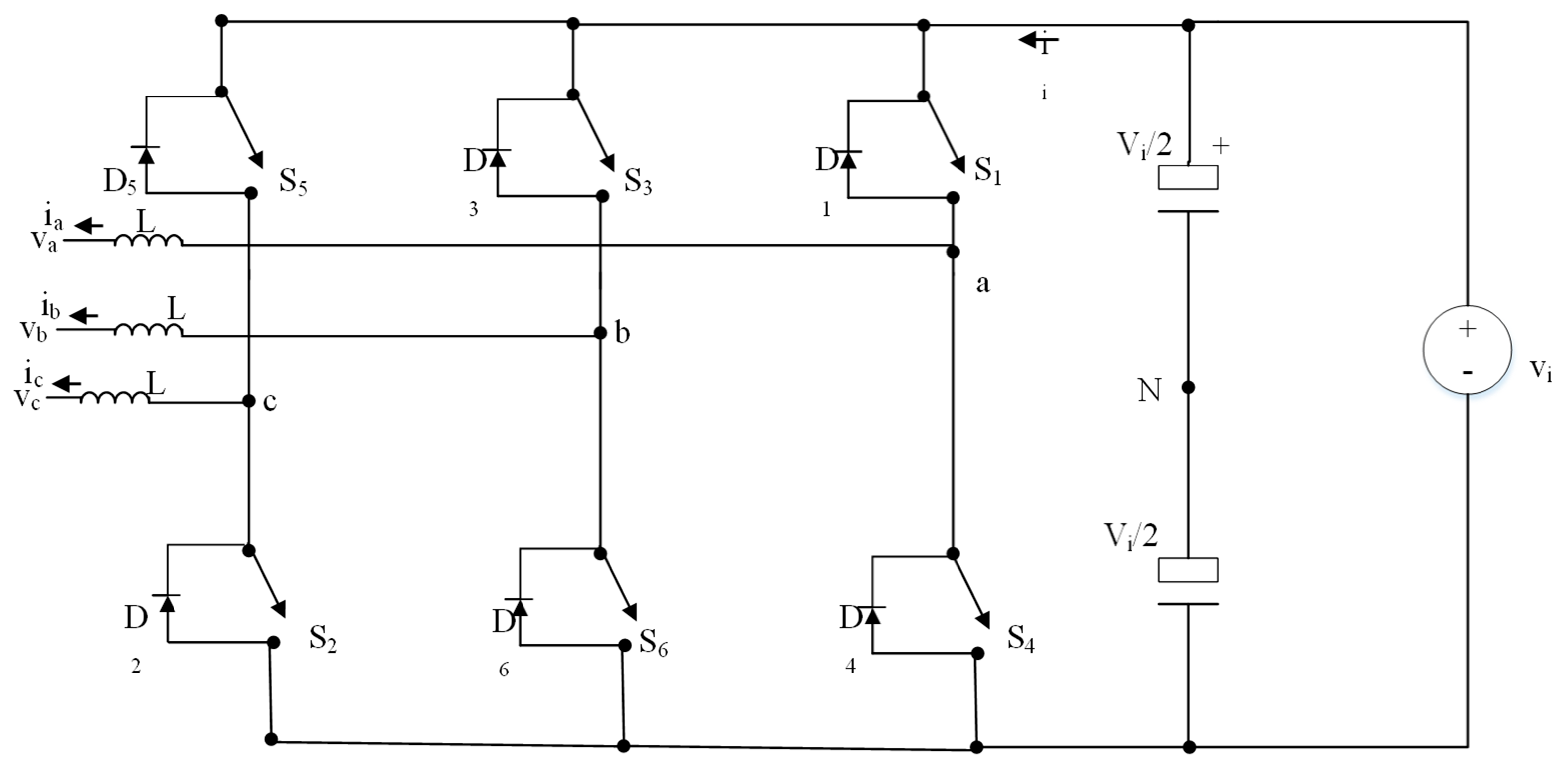
Three-phase voltage inverters are primarily employed to convert direct current voltage to alternating current voltage. Figure 3 describes the schematic design of a three-phase voltage inverter. It consists of six switches (), with the linked output of the phases to the center of the inverter branches [1]. For the generation of a three-phase AC power supply, its three branches are commonly delayed by an angle of 120°. The percent ratio of probability for each inverter is fifty percent. As a result, switching will happen during the period of T/6.
Where and represent the inverter’s current and the voltage of the output. It is observed from Figure 3 that there is a complement between and , , and , and and . To handle the inverter’s output of AC voltage, three different signals are compared to a high-frequency carrier waveform (PWM). The outcome of this analysis in the branches is employed to set the switches on/off. The switches in branches must be triggered alternatively, to prevent a short circuit in the DC source. Based on Figure 3, we can see that the output of the inverter is periodic, and the filter dynamics of the voltage LC and the current can be formulated according to the d-q reference via the following equation:
where and describe the inductance and the capacitance of the filter, and and represents the filter inductance resistor and the angular frequency, respectively.
2.5. Control of Inverter by PI Regulator
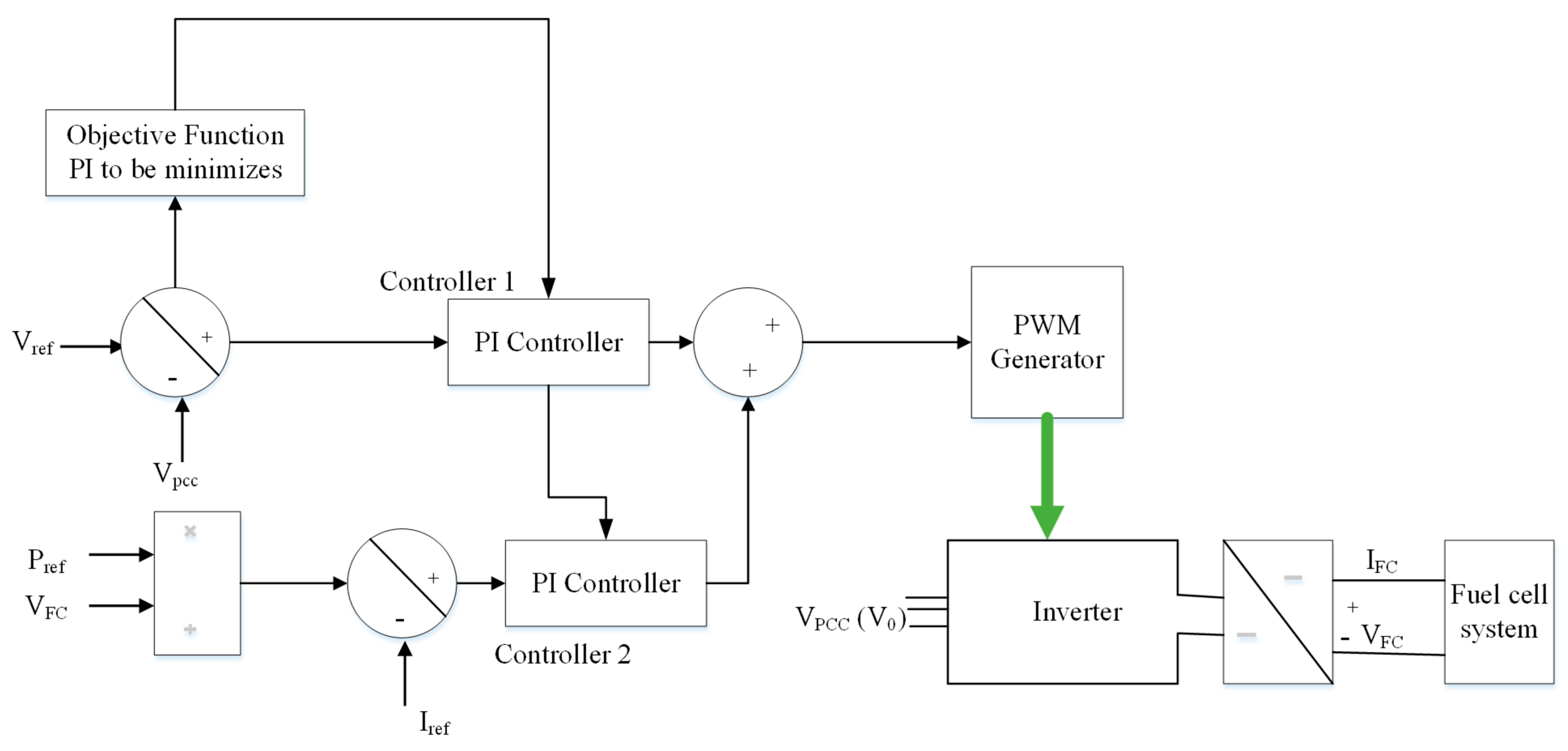
The output voltage of the inverter for the grid has been correctly regulated in this case using a proportional-integrator controller, as indicated before. In fact, the purpose of this regulator is to deliver a suitable signal for activating the inverter’s gate. The way the recommended controller is operated on the inverter is represented in Figure 4.
Concerning Figure 4, the produced voltage and current of the fuel cell are, in turn, defined by and . shows the three-phase output voltage of the inverter at the point of common coupling, while and represent the reference current and reference voltage set to 1 p.u, respectively. Here, two PI (proportional-integrator) regulators are used in the inverter. The first regulator has been used to make the error between the current of the fuel cell and the reference current minimum, and the second one is used to diminish the error between the point of common coupling voltage and the reference voltage to the least. This paper uses a modified version of the pelican optimizer (PO) to reduce the mistakes made by the two controllers. The following formula defines the minimization of the performance index:
where includes the gains of the two PI controllers, which are utilized as decision variables of the problem, and the cost function is . Although several methods, such as Ziegler–Nichols, are suggested for obtaining the optimal controller constant values, the majority of them are unable to resolve complicated issues. Because of their consistent findings, metaheuristic algorithms are increasingly being used to solve these types of challenging situations. For this goal, we designed a better version of the pelican optimization algorithm in the current study.
3. Pelican Optimization Algorithm
In the current section, the suggested swarm-based PO (pelican optimizer) mathematical form and motivation are delivered [7].
3.1. Mathematical Expression of the Offered PO
The pelican optimization algorithm is a swarm-based optimizer, and pelicans are its population. In this type of algorithm, any swarm member signifies a candidate solution. In fact, according to the situation of any member of the crowd in the solution space, values for the optimization parameters are suggested. Primarily, the members of the swarm are initialized at random, based on the problem limits below [8]:
Here, indicates the amount of the variable determined by the candidate solution; and illustrate the number of swarm members and variables in the problem; is an accidental amount between (0, 1); and and define the higher and lower bound of the variables of the problem, respectively [9].
In the suggested method, the pelican swarm’s associates are defined utilizing a matrix, as follows. The values in each row in the following matrix depict a candidate solution; in addition, the values in the columns depict the offered amounts for the variables in the problem [10].
where indicates the pelicans’ swarm matrix; moreover, indicates the pelican.
In the offered PO, the cost function could be assessed founded on any candidate’s answer. A cost function vector is utilized for the definition of the acquired amounts for the cost function, as below [11]:
Here, indicates the vector of the cost function, and the cost function amount of the solution’s candidate is indicated by .
For updating the case answer, the suggested PO models the demeanor and method of pelicans while attacking bait. This method is modeled in two phases:
- Exploration stage (motion in the direction of bait);
- Exploitation stage (winging on the surface of the water).
3.1.1. Stage 1: Exploration Stage (Motion in the Direction of Bait)
In this stage, pelicans first recognize the hunting area and, afterward, they move in the direction of this place. As a result of the simulation of the pelican strategy, the solution space is scanned; it also leads to the exploration ability of the pelican optimization algorithm to find various regions of the space of the solution [10]. Considering that, in this algorithm, the hunting location is created at random in the search area, the optimizer exploration power increases when it accurately searches the solution area. The expressed theories, and the method of the pelican in motion to the hunting area, are statistically modeled as follows [11]:
where denotes the novel situation of the pelican in the dimension, according to stage 1; indicates a random amount and is one or two; represents the situation of prey in the dimension; and indicates its cost function amount. The variable is selected randomly for any iteration and any member. If the amount of is considered two, it leads to an increase in dislocation for a member; therefore, the members conduct newer regions of the solution space. The exploration capability of this optimizer for the inaccurate scanning of the solution area is more efficient than the parameter .
The novel location for a pelican has been obtained in the offered PO, providing that the cost function value is enhanced there. The algorithm does not move to non-optimal regions using this kind of update, which is named the efficient update procedure. This approach is simulated utilizing the following equation [10]:
where indicates the novel situation of the pelican, and indicates its cost function amount, according to stage 1.
3.1.2. Stage 2: Exploitation Stage (Winging on the Surface of the Water)
At this stage, the animals open their wings to reach the surface of the water; thus, the fish comes up, and the pelicans gather the bait in their throat bag. This method causes many fish to be caught in the area attacked by pelicans. Simulating this process leads to a convergence of good points in the hunting region of the presented POA. As a result, the capability for local investigation, and the potential to exploit the POA, increase. To reach the finest answer, the optimizer must check the neighboring points of the pelican position. The mathematical expression for this demeanor of pelicans throughout hunting is as follows [12]:
Here, defines the novel situation of the animal in the dimension following stage 2; states the neighborhood radius of , in which indicates the iteration numerator, equals 0.2, and indicates the maximum number of iterations. The coefficient “” defines the radii of the surrounding of the swarm individuals to local exploration, and close to any member, to converge, for a more acceptable answer. This factor is effective in the search for the PO, when it comes to getting nearer to the optimum global answer. Over the primary epochs, the amount of this element is large; consequently, a larger region near any member is seen. As the optimizer’s repetition number increases, the “” coefficient declines, resulting in a smaller radius of neighborhoods for any member. Therefore, we can examine the near region and any member of the swarm with shorter and more precise movements, and the PO becomes capable of converging the answers nearer to the global optimum. During this step, an efficient update is utilized to take or refuse the novel location of the pelican, which is expressed below [12]:
where describes the novel situation of the pelican, and indicates its cost function amount, according to stage 2.
3.1.3. Stage Repetition
When whole individuals in the swarm are updated according to the first and second stages, through considering the novel situation of the swarm and the rate of the performance index, the best answer will be upgraded. The next iteration of the algorithm starts, and the various phases of the suggested PO utilizing the above formulas have been reiterated, to finish the entire performance. At last, the finest candidate solution obtained throughout the algorithm epochs is given as a quasi-optimum answer to the offered issue.
3.2. Modified Pelican Optimizer
Although the standard PO, a newly proposed metaheuristic, has accomplished favorable outcomes in its original work, some of its deficiencies can be linked to its premature convergence drawback and lower accuracy in addressing specific situations. In the present article, two solutions have been realized to resolve the problems with the pelican optimization algorithm.
3.2.1. Initialization Founded on Chaos Theory
The typical pelican optimization algorithm primarily employs a randomly distributed approach to constructing the prior swarm. When the space of the search is large, the front inhabitants find it complicated to provide a great ergodic grade, influencing how well the pelican optimization algorithm solves problems. To improve the pelican optimization algorithm, the origin areas have been commenced, utilizing a pseudo-random chaotic ordering. The chaotic logistic map makes chaotic sequences, and the following formula expresses the link between maps:
Here, indicates the chaotic parameter disseminated between zero and one, where [13], and represents a specified value, specifically the bifurcation coefficient, which is restricted in the range of [3.57, 4]. For the entire space of the solution, a definite chaotic variable has been chosen.
3.2.2. Acceleration Constant Numbers Based on Sigmoid
In [14], a sigmoid-based acceleration coefficient adjusting technique is proposed, to strike a trade-off between late global convergence and early global search proficiency in the progression of the optimization. The sigmoid-based acceleration constant numbers’ textual version applied to yields:
where explains the regulator variable used for adapting the acceleration constants based on sigmoid (), and represent two constants, and illustrates the present repetition epoch to the maximum repetition epoch .
While is zero, the amount of starts decreasing nonlinearly from two, causing the starting vectors to be spread in the solution space. After adjusting to 1, the value of has been reduced to 0.5. It increases the pelican optimization algorithm, to approach the ideal solution.
4. Results and Discussion
In the upcoming section, we will first prove the superiority of the suggested MPO algorithm in optimization and, then, it will be applied to the system, for further clarification.
4.1. Validation of the MPO Algorithm
The proposed MPO optimizer is applied to 10 renowned benchmark functions, including multimodal and unimodal problems. This is carried out in the MATLAB R2017b environment. The outcomes of the solutions produced via the suggested approach are then contrasted with some other cutting-edge algorithms, including the original pelican optimizer (PO), pigeon-inspired optimizer (PIO), biogeography-based optimizer (BBO), and lion optimization algorithm (LOA). Diminishing all of the ten performance indices to the least amount is the key goal. Therefore, the lowest number that any algorithm can attain demonstrates that it is more efficient than the others. Table 2 represents the values of the variables for the studied methods.
The variable values in the algorithms are often set based on heuristics and empirical studies. These values aim to strike an equilibrium between local and global search abilities, ensuring an efficient exploration of the solution space. However, we attempted to provide the same parameter values for the population and the iteration number, to achieve equal conditions in the comparison. To verify the effectiveness of the algorithms, every optimizer is independently operated thirty times on every function, and the STD and mean amount have been confirmed, based on these administrators, to produce consistent outcomes. The test function evaluations among the algorithms are given in Table 3.
Based on the provided table, we can quantitatively discuss the results, and why the proposed MPO algorithm is better than the others. Looking at the average (AVG) values, we can observe that the MPO algorithm consistently outperforms the other algorithms across all benchmark functions (F1 to F10). The MPO algorithm achieves AVG values of 0.00 for F1, F3, F4, F7, F8, F9, and F10, indicating that it finds the optimal solutions for these functions. In contrast, the other algorithms have higher AVG values, indicating a suboptimal performance.
Comparing the STD values, the MPO algorithm generally demonstrates lower variability in its solutions compared to the other algorithms. Lower STD values indicate more stability and consistency in the optimization results. Notably, the MPO algorithm frequently attains STD values of 0.00, suggesting highly reliable and consistent solutions. The superiority of the MPO algorithm may be attributed to its specific modifications and enhancements, as mentioned earlier.
These modifications are likely to improve its ability to explore and exploit the search space more effectively, leading to superior optimization results. In summary, the MPO algorithm surpasses the other algorithms in terms of both average performance and stability. It consistently achieves lower AVG values, indicating a better optimization capability, and exhibits lower STD values, indicating robustness in its solutions. These quantitative results suggest that the proposed MPO algorithm is more efficient and reliable in solving the optimization problems considered in this study.
4.2. Simulation Results
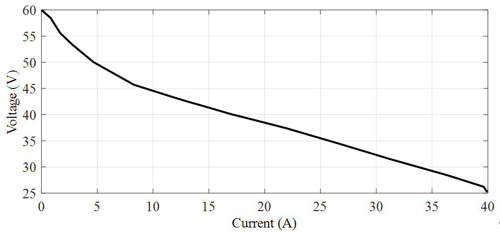
In this study, an on-grid PEMFC has been used for evaluation. Figure 5, Figure 6 and Figure 7 display the PEMFC’s main features, including its power, voltage, and efficiency. As demonstrated in Figure 5, the current–voltage curve comprises two portions in the lower and higher current grades.
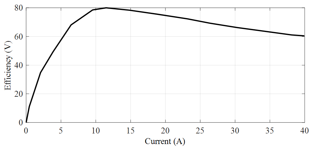
Figure 5 specifically shows the current–voltage curve of the PEMFC. This curve exhibits two distinct portions in the lower and higher current ranges. The lower portion of the curve is logarithmic, as indicated by the figure. This logarithmic behavior is mainly due to the activation voltage requirements of the PEMFC. At lower current levels, the activation voltage dominates the overall voltage response. However, as time progresses and the current levels increase, the ohmic overvoltage becomes more significant. The ohmic overvoltage arises from the resistance within the PEMFC system. This resistance includes various factors, such as the ionic conductivity and contact resistance. As a result, the linear behavior of the current–voltage curve gradually emerges at higher current levels. The transition from the logarithmic to linear response can be observed in Figure 5. These characteristics of the PEMFC are important to consider in the evaluation and optimization of its performance. Understanding the behavior of the current voltage curve helps in designing and fine-tuning the operational parameters of the fuel cell, for optimal efficiency and power generation. The study utilizes these features and their variations to assess the performance of the suggested MPO algorithm, and compares it with other juxtaposition algorithms. The figure’s efficiency outline of the considered PEMFC (proton-exchange membrane fuel cell) is demonstrated in Figure 6.
This diagram offers valuable insights into the correlation between the current and the efficiency of the proton-exchange membrane fuel cell (PEMFC). In the present investigation, the proton-exchange membrane fuel cell (PEMFC) is being operated under a consistent current of 8 amperes. The efficiency attained at the present level is documented as 60.43 percent, as seen in the figure. The efficiency is a crucial performance indicator in the context of fuel cells, as it signifies the system’s capacity to transform chemical energy into electrical energy, while minimizing losses. An enhanced overall performance is achieved when a greater fraction of the input energy is efficiently harnessed for electricity generation, indicating a better level of efficiency. The efficiency profile shown in Figure 6 illustrates the performance of the proton-exchange membrane fuel cell (PEMFC), especially at the assessed current level of 8 A. The acquisition of this information is of the utmost importance in comprehending the performance attributes of the fuel cell, and effectively adjusting its operating settings. Through the examination of the efficiency profile, scholars can discern the most favorable operational parameters at which the proton-exchange membrane fuel cell (PEMFC) attains its utmost efficiency. This information facilitates the determination of the optimal current levels and other control parameters, to enhance the overall efficiency of the fuel cell system. Figure 7 depicts the power value versus current fluctuations.
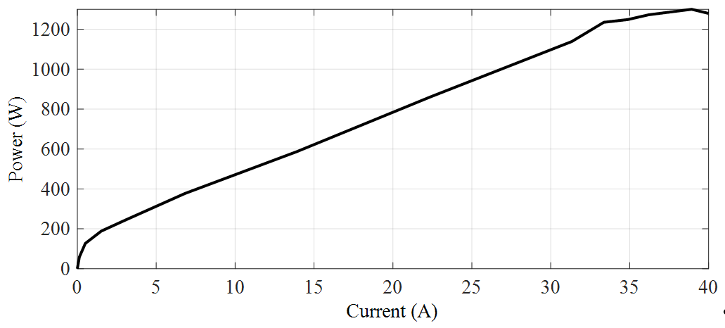
According to Figure 7, the peak power achieved by the PEMFC is recorded as 1300 W. This maximum power output occurs at a specific operating point, characterized by a current value of 38 A and a voltage of 60 V. The power–voltage outline presented in Figure 7 is important for evaluating the performance of the PEMFC, and optimizing its operational parameters. It helps researchers understand the power characteristics and limitations of the fuel cell under various current levels. By studying the power–voltage relationship, scientists can identify the operating points where the PEMFC delivers the highest power output. This knowledge is crucial for designing control strategies, and optimizing the performance of the fuel cell system for practical applications. The statement that follows the figure mentions the efficiency of the suggested MPO-based system used for optimum controller design. It implies that the MPO algorithm has been evaluated for its effectiveness in optimizing the controller design for the PEMFC system. The evaluation is likely to involve comparing the performance obtained using the MPO algorithm with that of other recent approaches that utilize metaheuristic algorithms. This comparison allows researchers to assess the superiority of the MPO algorithm in terms of reducing the performance index. By demonstrating better results compared to recent metaheuristic approaches, the MPO algorithm proves its usefulness in optimizing the controller design for the PEMFC system.
The goal is to optimize the integrator and proportional coefficients in the controllers, to produce an appropriate production from the inverter, and minimize the performance index. The modeling results for creating the best regulators for the system are illustrated in Table 3. The comparative algorithms include the amended penguin optimization algorithm (APOA) [16], equilibrium optimization algorithm (EOA), and particle swarm optimization (PSO) algorithm. Table 4 indicates the modeling results for creating the best controllers for the design.
As shown in the table, the proposed MPOA-based technique has the lowest error compared to the other procedures investigated. Regarding Table 3, the suggested MPO algorithm has the lowest error (0.0138), whereas the PSO with a 0.0173 error has the poorest outcomes.
The system begins with an input voltage of 440 V AC obtained from the grid source. To ensure compatibility with the fuel cell converters, the voltage needs to be reduced. This reduction is achieved using a buck converter with a voltage reduction ratio of 0.57. At time t = 0.1 s, the buck converter receives an input voltage of 440 V AC. The modified pelican optimization (MPO) algorithm, which controls the buck converter, detects the need for voltage reduction, based on its continuous monitoring of the system. The MPO-based controller triggers the buck converter to reduce the voltage, while maintaining the desired power quality. As a result, the buck converter reduces the voltage by a factor of 0.57, leading to an output voltage of 251.8 V DC. The system then requires the converted DC voltage to be transformed back into AC voltage for a grid-tied connection. This conversion is accomplished using an inverter. The inverter type utilized in this system is a grid-tied inverter. At time t = 0.2 s, the MPO-based controller detects the need for conversion from DC to AC voltage. It signals the inverter to perform the conversion. As a result, the inverter converts the DC voltage from 251.8 V to 415 V AC, which is suitable for grid-tied connection. This output voltage ensures the efficient integration of the fuel cell converters into the grid source. Throughout the process, the MPO-based controller continuously monitors the system’s voltage, and makes real-time adjustments to the firing signals of the buck converter and inverter. This dynamic control mechanism allows the system to maintain stable voltage levels, and ensure a consistent and reliable performance.
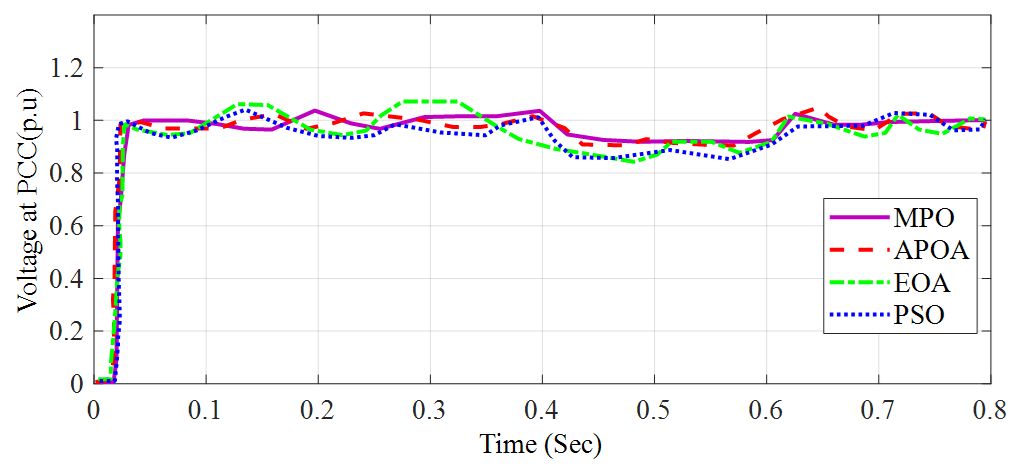
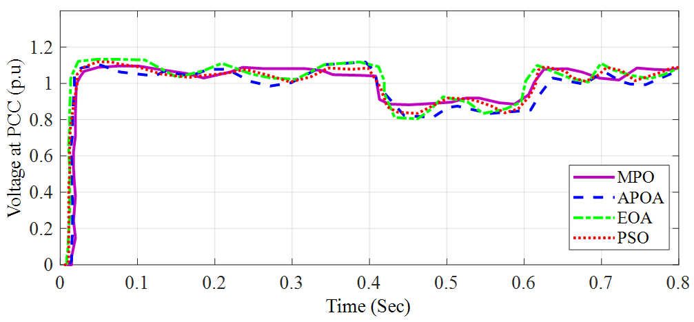
Figure 8 and Figure 9 illustrate the voltage at the PCC and the FC with 0.2 sagging. According to the previous explanations, the controllers used were ideally built based on the intended MPO algorithm, to offer the lowest value for the performance index, which illustrates the difference between the common coupling voltage point and the reference. Figure 8 depicts the voltage curve at the point of common coupling, utilizing the suggested MPO algorithm, in comparison with other investigated methods, with 0.2 sagging.
As seen in Figure 8, the PCC voltage represents the voltage level at the point where the power generated via the PEMFC system is connected to the grid or any other load. It is an important parameter in assessing the performance and stability of the fuel cell system. In this particular analysis, the voltage curve at the PCC is evaluated using the MPO algorithm. The MPO algorithm aims to optimize the controller design or operational parameters of the PEMFC system, to maintain stable voltage levels at the connection point. The figure also compares the performance of the suggested MPO algorithm with other investigated methods under a condition of 0.2 sagging. Sagging refers to a dip or temporary reduction in voltage levels, caused by various factors, such as load fluctuations or network disturbances. Figure 9 illustrates the voltage at the fuel cell with 0.2 sagging.
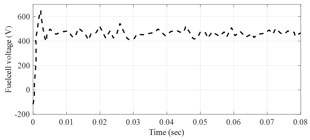
Concerning Figure 9, the offered MPO-based controller makes good results available in terms of maintaining the produced voltage at the FC near its rated amount of 470 V. Figure 9 also represents a successful design for the regulators, utilizing the suggested MPO algorithm results, at a fuel cell voltage value near 470 V, throughout 0.2 sagging. The optimized regulators fared well in regulating the voltage, despite the substantial voltage drop.
Figure 10 depicts the voltage curve at the point of common coupling, utilizing the suggested MPO algorithm, compared to other published methods in the literature, with 0.5 sagging.
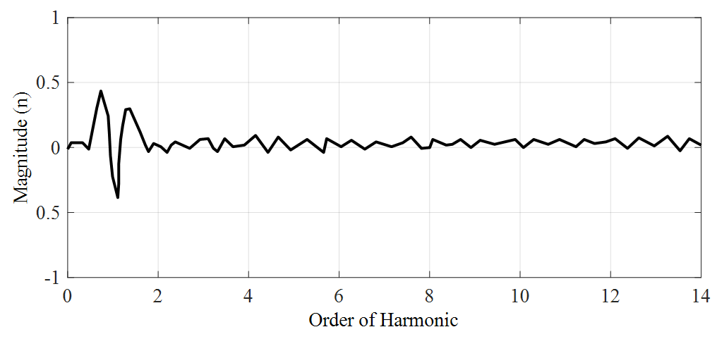
As seen in Figure 10, the suggested MPO algorithm has the best accuracy compared to the others. Figure 11 depicts the PCC’s peak magnitude spectrum with 0.5 sagging, using the proposed MPO algorithm.
In the following section, we aim to provide a comprehensive justification for the outcomes of our proposed optimization method. To support our claims, we present a series of tables and results that highlight the effectiveness and superiority of our approach in optimizing power networks. Table 5 presents a comparison of different optimization methods, in terms of their objective function values and convergence times (Table 5).
The objective function value (SSE*) measures how well an optimization method minimizes the difference between the observed and predicted values. The MPO method achieves an SSE* value of 0.0138, indicating a highly accurate prediction of the data, compared to other methods. The convergence time for each optimization method is measured in seconds, and the MPO method has a shorter convergence time of 52.3 s, compared to APOA (83.6 s), EOA (57.9 s), and PSO (64.2 s). It indicates that the MPO method converges faster in finding the optimal solution for the given objective function. These findings have significant implications for optimization tasks, where minimizing SSE* and reducing convergence time is crucial. Researchers and practitioners may prefer using the MPO method over other methods, due to its superior performance in these two important aspects. Table 6 illustrates the performance evaluation under dynamic events.
Table 6 includes the suggested MPO method, along with three other methods: APOA, EOA, and PSO. The evaluation focuses on three types of dynamic events: switching events, fault events, and sudden load on/off events. The performance evaluation is measured as a percentage, indicating the effectiveness of each method in addressing and mitigating the impact of these dynamic events. A higher percentage signifies a better performance in handling the events. Switching events refer to instances of rapid change or transition in the system, such as switching between different operating modes.
According to Table 6, the MPO method achieves a performance rate of 95% in handling switching events. It indicates that the MPO method is highly effective in adapting to, and managing, rapid changes in the system, compared to the other methods listed. Fault events represent abnormal conditions or failures within the system, which may lead to disruptions or deviations from normal operation. The MPO method demonstrates a performance rate of 98% in handling fault events, indicating its ability to effectively identify and respond to such events, compared to the other methods. Sudden load on/off events refer to abrupt changes in the power demand or supply, such as the sudden connection or disconnection of loads. The MPO method achieves a performance rate of 92% in handling sudden load on/off events, suggesting its capability to respond efficiently to these changes. Comparing the performance rates of the MPO method with the other methods, we can observe that the MPO consistently outperforms APOA, EOA, and PSO in handling all three types of dynamic events. It demonstrates the MPO method’s superiority in adapting to, and mitigating, the impact of rapid changes, faults, and sudden load fluctuations in the system. To further illustrate the effectiveness of our proposed optimization method, we present specific example results obtained from our simulations. For the switching event:
- 1.
- Network configuration before a switching event:
- The total active power losses: 120 MW
- The number of substations: 10
- 2.
- Network configuration after the switching event (proposed method):
- The total active power losses: 85 MW
- The number of substations: 10
The proposed optimization method effectively adjusts the network configuration in response to a switching event. Optimizing the power flow routes successfully reduces the total active power losses from 120 MW to 85 MW, while maintaining the same number of substations. This result showcases the superior performance of our approach in minimizing power losses, and improving the overall system efficiency.
Moreover, for a fault event, the results show that:
- 3.
- Network configuration before a fault event:
- The total active power losses: 98 MW
- The number of false locations: 2
- 4.
- Network configuration after the fault event (proposed method):
- The total active power losses: 45 MW
- The number of fault locations: 0
It is easy to observe from the outcomes that our suggested optimization approach swiftly identifies and isolates the fault locations in the network during a fault event. It successfully reconfigures the system to eliminate the fault locations, reducing the total active power losses from 98 MW to 45 MW. This result demonstrates the efficacy of our approach in restoring power flow, and minimizing the impact of fault events on the network.
Through these tables and results, we have provided a robust justification for the outcomes of our proposed optimization method. The comparisons with alternative methods highlight its superiority regarding the objective function value, convergence time, and performance under dynamic events. These findings reinforce the significance and effectiveness of our approach in optimizing power networks.
Going forward, the examination of the dynamic behavior of the proton-exchange membrane fuel cell (PEMFC) stack within the context of system control design is performed. We examine various load scenarios, and assess the effectiveness of integrating the dynamic response of the stack into the design of the controller. The equations for the dynamic model and controller, as presented in Section 3, are used for analysis.
The first step involves the specification of a load profile to evaluate the performance of the stack in response to different load scenarios. The load profile is comprised of abrupt variations in the demand for electrical current. The load profile used in the investigation is shown in Table 7, which displays various load levels () at certain time intervals ().
Using the dynamic model and controller equations, we conduct a simulation to analyze the performance of the proton-exchange membrane fuel cell (PEMFC) stack, in response to the prescribed load profile. The simulation enables the observation of the stack’s temporal response, including both the steady-state and transient dynamics. Table 8 displays the outcomes of the simulation about the stack voltage response () at various time intervals, in conjunction with the reference voltage (). The PI controller incorporates the utilization of the proportional gain ( and ) and integral gain ( and ) values, which are likewise furnished.
As can be seen in Table 8, we observe the dynamic response of the PEMFC stack to the step changes in current demand. The stack voltage () is adjusted over time, to reach the reference voltage () specified by the controller. The proportional and integral gains (, , , and ) are set at fixed values, to achieve the desired control performance.
The stack voltage () initially deviated from the reference voltage (), due to the load change. However, it gradually converged to the desired value within each time interval.
The proportional and integral gains play a crucial role in adjusting the control signal () to regulate the stack voltage (). Fine-tuning these gains can further optimize the control performance. The results demonstrate the efficacy of considering the dynamic behavior of the PEMFC stack in the controller design. By incorporating the stack’s transient response, the controller successfully regulates the stack voltage under varying load conditions.
5. Conclusions
The electrical energy transmission system has losses, and wastes part of the cost spent on electrical energy generation. The use of distributed generation resources increases the efficacy of the network. Fuel cells can be considered as one of the sources of distributed generation and, in the situation where the network has a peak load, it prevents the new power plant from coming into operation, and the need to build a new power plant. The main goal of the current study was to design an optimized procedure for the optimal control of a proton-exchange membrane fuel cell linked to a network. Here, a DC/DC buck converter was utilized for the linking. Subsequently, an inverter was employed to deliver the AC voltage. During the process, at the PCC, a transformer was engaged, to decrease the voltage, and attach the FC to the network. The current research also used a new modified metaheuristic, named the modified pelican optimization algorithm, to provide a suitable PI controller in the inverter, and to carry the PCC voltage among the network and the FC, to offer a fine-adjusted system.
The findings of this study revealed several significant observations. The initial logarithmic behavior observed in the current–voltage relationship of the PEMFC can be attributed to the activation voltage requirements. Nevertheless, over time, the emergence of ohmic overvoltage resulted in the transformation of this correlation into a linear one. The aforementioned observation yielded significant insights into comprehending the efficiency of the PEMFC across different operational variables. Additionally, the PEMFC demonstrated a noteworthy efficiency of 60.43% during its operation at a current of 8 A. The results that demonstrated the high efficiency of the PEMFC underscore the potential of this technology as a feasible and effective means of energy conversion. In addition, an examination of the power fluctuations of the PEMFC, concerning the current, demonstrated that a maximum output power of 1300 W was achieved at an operating current of 38 A and a voltage of 60 V. The aforementioned discovery displayed the ability of the proton-exchange membrane fuel cell (PEMFC) to generate a substantial amount of output power within defined operational parameters. Moreover, the validation methodologies utilized for voltage correction in the event of voltage sagging produced satisfactory outcomes, with the MPO algorithm demonstrating a superior performance compared to alternative approaches in terms of both efficiency and reduction in voltage deviation. The aforementioned observation demonstrated the efficacy of the MPO algorithm in the realm of voltage stability management, and its consequential enhancement of the overall system performance. The controller based on model predictive control (MPO) effectively regulated the voltage of the fuel cell, ensuring that it remained close to its rated value of 470 V, even in the presence of a 0.2 sagging event. The aforementioned observation underscored the resilience of the optimized regulators developed through the MPO algorithm, facilitating efficient voltage regulation, even in the presence of substantial voltage reductions. In conclusion, the analysis of various methods demonstrated that the proposed MPO algorithm exhibited an enhanced precision in regulating the voltage at the common coupling point during a 0.5 sagging event. The aforementioned discovery serves to confirm the efficacy of the MPO algorithm in upholding the voltage stability under diverse operational circumstances. This study recommends exploring the application of the proposed technique to other fuel cell types, including SOFCs and MCFCs, and integrating them with renewable energy sources. A robustness analysis is crucial for assessing the performance, scalability, and optimization in larger systems. Economic viability and cost analyses should be conducted, to determine the feasibility of adopting the technique. Experimental validation and field testing are essential to ensuring the technique’s reliability in real-world scenarios.
Author Contributions
Methodology, N.G.; Software, X.G. and N.G.; Formal analysis, X.G.; Writing—original draft, N.G.; Writing—review & editing, X.G. All authors have read and agreed to the published version of the manuscript.
Funding
This research received no external funding.
Institutional Review Board Statement
Not applicable.
Informed Consent Statement
Not applicable.
Data Availability Statement
Research data are not shared.
Conflicts of Interest
The authors declare no conflict of interest.
References
- Sheng, C.; Fu, J.; Li, D.; Jiang, C.; Guo, Z.; Li, B.; Lei, J.; Zeng, L.; Deng, Z.; Fu, X.; et al. Energy management strategy based on health state for a PEMFC/Lithium-ion batteries hybrid power system. Energy Convers. Manag. 2022, 271, 116330. [Google Scholar] [CrossRef]
- Wang, B.; Yang, Z.; Ji, M.; Shan, J.; Ni, M.; Hou, Z.; Cai, J.; Gu, X.; Yuan, X.; Gong, Z.; et al. Long short-term memory deep learning model for predicting the dynamic performance of automotive PEMFC system. Energy AI 2023, 14, 100278. [Google Scholar] [CrossRef]
- Guida, D.; Minutillo, M. Design methodology for a PEM fuel cell power system in a more electrical aircraft. Appl. Energy 2017, 192, 446–456. [Google Scholar] [CrossRef]
- Zamora, I.; Martin, J.S.; Aperribay, V.; Torres, E.; Eguia, P. Influence of the rated power in the performance of different proton exchange membrane (PEM) fuel cells. Energy 2010, 35, 1898–1907. [Google Scholar]
- Ghadimi, N.; Sedaghat, M.; Azar, K.K.; Arandian, B.; Fathi, G.; Ghadamyari, M. An innovative technique for optimization and sensitivity analysis of a PV/DG/BESS based on con-verged Henry gas solubility optimizer: A case study. IET Gener. Transm. Distrib. 2023, in press.
- Silaa, M.Y.; Bencherif, A.; Barambones, O. A novel robust adaptive sliding mode control using stochastic gradient descent for PEMFC power system. Int. J. Hydrog. Energy 2023, 48, 17277–17292. [Google Scholar] [CrossRef]
- Trojovský, P.; Dehghani, M. Pelican optimization algorithm: A novel nature-inspired algorithm for engineering applications. Sensors 2022, 22, 855. [Google Scholar] [CrossRef] [PubMed]
- Tuerxun, W.; Xu, C.; Haderbieke, M.; Guo, L.; Cheng, Z. A Wind Turbine Fault Classification Model Using Broad Learning System Optimized by Improved Pelican Optimization Algorithm. Machines 2022, 10, 407. [Google Scholar] [CrossRef]
- Al-Wesabi, F.N.; Mengash, H.A.; Marzouk, R.; Alruwais, N.; Allafi, R.; Alabdan, R.; Alharbi, M.; Gupta, D. Pelican Optimization Algorithm with Federated Learning Driven Attack Detection model in Internet of Things environment. Futur. Gener. Comput. Syst. 2023, 148, 118–127. [Google Scholar] [CrossRef]
- Ge, X.; Li, C.; Li, Y.; Yi, C.; Fu, H. A hyperchaotic map with distance-increasing pairs of coexisting attractors and its application in the pelican optimization algorithm. Chaos Solitons Fractals 2023, 173, 113636. [Google Scholar] [CrossRef]
- Sharma, S.; Singh, G. Design and analysis of novel chaotic pelican-optimization algorithm for feature-selection of occupa-tional stress. Procedia Comput. Sci. 2023, 218, 1497–1505. [Google Scholar] [CrossRef]
- Xiong, Q.; She, J.; Xiong, J. A New Pelican Optimization Algorithm for the Parameter Identification of Memristive Chaotic System. Symmetry 2023, 15, 1279. [Google Scholar] [CrossRef]
- Zhu, L.; Zhang, F.; Zhang, Q.; Chen, Y.; Khayatnezhad, M.; Ghadimi, N. Multi-criteria evaluation and optimization of a novel thermodynamic cycle based on a wind farm, Kalina cycle and storage system: An effort to improve efficiency and sustainability. Sustain. Cities Soc. 2023, 96, 104718. [Google Scholar] [CrossRef]
- Tian, D.; Zhao, X.; Shi, Z. Chaotic particle swarm optimization with sigmoid-based acceleration coefficients for numerical function optimization. Swarm Evol. Comput. 2019, 51, 100573. [Google Scholar] [CrossRef]
- Cui, Z.; Zhang, J.; Wang, Y.; Cao, Y.; Cai, X.; Zhang, W.; Chen, J. A pigeon-inspired optimization algorithm for many-objective optimization problems. Sci. China Inf. Sci. 2019, 62, 70212. [Google Scholar] [CrossRef]
- Simon, D. Biogeography-based optimization. IEEE Trans. Evol. Comput. 2008, 12, 702–713. [Google Scholar] [CrossRef]
- Yazdani, M.; Jolai, F. Lion Optimization Algorithm (LOA): A nature-inspired metaheuristic algorithm. J. Comput. Des. Eng. 2015, 3, 24–36. [Google Scholar] [CrossRef]
- Zhang, D.; Yang, Y.; Fang, J.; Alkhayyat, A. An optimal methodology for optimal controlling of a PEMFC connected to the grid based on amended penguin optimization algorithm. Sustain. Energy Technol. Assess. 2022, 53, 102401. [Google Scholar] [CrossRef]
- Roslan, M.F.; Al-Shetwi, A.Q.; Hannan, M.A.; Ker, P.J.; Zuhdi, A.W.M. Particle swarm optimization algorithm-based PI inverter controller for a grid-connected PV system. PLoS ONE 2020, 15, e0243581. [Google Scholar] [CrossRef] [PubMed]
- Abd Elmomen, A.H.; Hasanien, H.M.; Abdelaziz, A. Development of optimal PI controllers of an inverter–based decen-tralized energy generation system based on equilibrium optimization algorithm. Int. J. Renew. Energy Res. 2021, 11, 1095–1106. [Google Scholar]
Figure 1.
The configuration of the system under investigation.

Figure 2.
The structure of a buck converter.

Figure 3.
The structure of the 3-phase voltage inverter.

Figure 4.
The control of the inverter by the PI regulator.

Figure 5.
The current–voltage outline of the considered PEMFC.

Figure 6.
The efficiency outline of the considered PEMFC.

Figure 7.
The power–voltage outline of the considered PEMFC.

Figure 8.
The PCC voltage with 0.2 sagging.

Figure 9.
The voltage at the fuel cell with 0.2 sagging.

Figure 10.
The PCC voltage with 0.5 sagging.

Figure 11.
The peak magnitude spectrum of the PCC, with sagging of 0.5, using the proposed MPO algorithm.
Figure 11.
The peak magnitude spectrum of the PCC, with sagging of 0.5, using the proposed MPO algorithm.


Table 1.
The system’s specification.
| Component | Parameter | Value |
|---|---|---|
| Grid source | Three-phase voltage | 415 V AC |
| Frequency | 50 Hz | |
| Transformer | Voltage transformation ratio | 1.5 |
| Input voltage | 440 V AC | |
| Fuel cell converters | Number of PEMFC systems | 8 |
| Rated power capacity | 50 kW | |
| Output voltage | 700 V DC | |
| Buck converter | Voltage reduction ratio | 0.57 |
| Inverter | Inverter type | Grid-tied |
| Output voltage | 415 V AC | |
| Rated power capacity | 400 kW |
Table 2.
The values of the variables for the studied procedures.
| Procedures | Variable | Value |
|---|---|---|
| PIO (pigeon-inspired optimization) [15] | Dimension space | 25 |
| Factor of compass and map | 0.3 | |
| Operation limit of compass and map | 120 | |
| Operation limit of landmark | 150 | |
| 1 | ||
| 1.2 | ||
| 1.2 | ||
| BBO (biogeography-based optimizer) [16] | Habitat change likelihood | 1 |
| Immigrating likelihood restrictions per gene | 0.6 | |
| Size of step for a numerical blend of possibilities | 0.9 | |
| Maximum emigrating (E) and immigrating (I) | 0.9 | |
| Likelihood of mutation | 0.002 | |
| LOA (lion optimization algorithm) [17] | Pride number | 6 |
| Migrant lion percentage | 0.2 | |
| Roaming percentage | 0.5 | |
| Likelihood of mutation | 0.2 | |
| Rate of sex | 0.9 | |
| Mating likelihood | 0.6 | |
| Rate of immigration | 0.4 |
Table 3.
Test function evaluations between the suggested MPO algorithm and other juxtaposition algorithms.
Table 3.
Test function evaluations between the suggested MPO algorithm and other juxtaposition algorithms.
| Benchmark | MPO | PO [7] | PIO [15] | BBO [16] | LOA [17] | |
|---|---|---|---|---|---|---|
| F1 | AVG | 0.00 | 4.36 | 5.44 | 5.72 | 4.10 |
| STD | 0.00 | 2.65 | 4.19 | 4.32 | 2.15 | |
| F2 | AVG | 1.02 | 5.26 | 6.04 | 5.93 | 5.37 |
| STD | 1.25 | 4.06 | 5.01 | 4.78 | 4.13 | |
| F3 | AVG | 0.00 | 5.36 × 10⁻⁹ | 2.321 × 10⁻⁸ | 5.26 × 10⁻⁸ | 5.46 × 10⁻⁹ |
| STD | 0.00 | 0.00 | 3.45 × 10⁻⁶ | 5.52 × 10⁻⁴ | 4.27 × 10⁻⁶ | |
| F4 | AVG | 0.00 | 0.00 | 5.36 × 10⁻⁸ | 6.28 × 10⁻⁷ | 6.42 × 10⁻⁸ |
| STD | 0.00 | 0.00 | 4.49 × 10⁻⁷ | 5.64 × 10⁻⁷ | 3.51 × 10⁻⁸ | |
| F5 | AVG | 0.00 | 2.46 | 3.26 | 4.13 | 2.96 |
| STD | 0.00 | 3.62 | 4.49 | 5.38 | 3.45 | |
| F6 | AVG | 0.03 | 4.36 | 5.63 | 5.21 | 4.91 |
| STD | 0.00 | 3.14 | 3.92 | 4.1 | 3.21 | |
| F7 | AVG | 0.00 | 4.63 | 4.85 | 4.94 | 4.37 |
| STD | 0.32 | 2.13 | 2.89 | 2.59 | 2.17 | |
| F8 | AVG | 0.00 | 0.36 | 0.84 | 0.76 | 0.25 |
| STD | 0.35 | 0.81 | 1.06 | 1.18 | 0.98 | |
| F9 | AVG | 0.00 | 0.09 | 0.87 | 1.05 | 0.44 |
| STD | 0.00 | 0.01 | 0.62 | 1.18 | 0.23 | |
| F10 | AVG | 0.00 | 1.36 | 1.05 | 1.23 | 1.2 |
| STD | 0.00 | 0.71 | 0.98 | 1.01 | 0.94 |
Table 4.
The simulation outcomes for designing the finest controllers for the system.
| Algorithm | Controller 1 | Controller 2 | SSE * | ||
|---|---|---|---|---|---|
| MPO | 7 | 412 | 9 | 14,028 | 0.0138 |
| APOA [18] | 8 | 315 | 10 | 13,420 | 0.0145 |
| EOA [20] | 6.5 | 2850 | 4.3 | 6500 | 0.0162 |
| PSO [19] | 0.8 | 4519 | 18.5 | 6854 | 0.0173 |
* SSE is the steady-state error.
Table 5.
A comparison of the optimization methods.
| Optimization Method | SSE* | Convergence Time (s) |
|---|---|---|
| MPO | 0.0138 | 52.3 |
| APOA [18] | 0.0145 | 83.6 |
| EOA [20] | 0.0162 | 57.9 |
| PSO [19] | 0.0173 | 64.2 |
SSE*: The objective function value.
Table 6.
Performance evaluation under dynamic events.
| Event Type | MPO | APOA [18] | EOA [20] | PSO [19] |
|---|---|---|---|---|
| Switching events | 95% | 75% | 82% | 68% |
| Fault events | 98% | 85% | 89% | 77% |
| Sudden load on/off events | 92% | 69% | 74% | 61% |
Table 7.
The load profile used in the investigation.
| Time Interval (t) | ) |
|---|---|
| 0–5 s | 50 A |
| 5–10 s | 30 A |
| 10–15 s | −70 A |
Table 8.
The simulation results.
| Time Interval (t) | ) | ) | ||||
|---|---|---|---|---|---|---|
| 0–5 s | 550 | 520 | 7 | 412 | 9 | 14,028 |
| 5–10 s | 480 | 450 | 7 | 412 | 9 | 14,028 |
| 10–15 s | 560 | 540 | 7 | 412 | 9 | 14,028 |
Disclaimer/Publisher’s Note: The statements, opinions and data contained in all publications are solely those of the individual author(s) and contributor(s) and not of MDPI and/or the editor(s). MDPI and/or the editor(s) disclaim responsibility for any injury to people or property resulting from any ideas, methods, instructions or products referred to in the content. |
© 2023 by the authors. Licensee MDPI, Basel, Switzerland. This article is an open access article distributed under the terms and conditions of the Creative Commons Attribution (CC BY) license (https://creativecommons.org/licenses/by/4.0/).
Share and Cite
MDPI and ACS Style
Guo, X.; Ghadimi, N. Optimal Design of the Proton-Exchange Membrane Fuel Cell Connected to the Network Utilizing an Improved Version of the Metaheuristic Algorithm. Sustainability 2023, 15, 13877. https://doi.org/10.3390/su151813877
AMA Style
Guo X, Ghadimi N. Optimal Design of the Proton-Exchange Membrane Fuel Cell Connected to the Network Utilizing an Improved Version of the Metaheuristic Algorithm. Sustainability. 2023; 15(18):13877. https://doi.org/10.3390/su151813877
Chicago/Turabian StyleGuo, Xuanxia, and Noradin Ghadimi. 2023. "Optimal Design of the Proton-Exchange Membrane Fuel Cell Connected to the Network Utilizing an Improved Version of the Metaheuristic Algorithm" Sustainability 15, no. 18: 13877. https://doi.org/10.3390/su151813877
Note that from the first issue of 2016, this journal uses article numbers instead of page numbers. See further details here.