1. Introduction
The European and national regulatory framework in the decarbonization path towards 2050 highlights the role of district heating (DH) in achieving the goals of efficiency, energy sustainability, renewables, and reduction in fossil fuel use [
1]. The performance of the innovative configurations of the “efficient” networks are key topics in scientific research, focusing on distribution temperatures (low/neutral temperature DH) and on the integration of high-efficiency plants and additional sources [
2]. In this last case, the local production from renewable energy sources and/or waste heat recovery could be connected to the district heating network (DHN) by smart bidirectional substations, as stated in the European Directive 2018/2001/EU (so-called REDII) [
3]. As a consequence, thermal users characterized by the presence of distributed generators may operate as prosumers and feed the network with the surplus of heat production.
Relating to renewable-based technologies, solar (both thermal and photovoltaic, coupled with heat pumps) and geothermal systems are particularly attractive to be employed in smart bidirectional substations [
4,
5], especially in the context of low temperature DHN [
6]. On the other hand, waste heat recovery from data centers is an interesting solution for large scale prosumers [
7] since data centers are characterized by a great amount of waste heat with an almost stable profile during the day.
At present, however, while prosumers are widespread in the electricity sector—mainly thanks to the diffusion of distributed photovoltaic systems, as well as to the dedicated support schemes and a proper regulatory framework—they are uncommon in the DH sector [
8]. Nevertheless, the possibility of integrating distributed heat generation systems into DHNs has been deeply investigated in the literature. As an example, Brange et al. [
9] presented a case study in Malmö (Sweden), where small-scale thermal prosumers supply heat to a DHN with a heat pump (HP) or directly, with a potential excess heat around 50–120% compared to the annual heat demand. Furthermore, Kauko et al. [
10] evaluated different DH scenarios in Trondheim (Norway), including thermal prosumers connected to a low-temperature DHN; the study demonstrates that a reduction of up to 25% can be achieved in the heat demand from the central heating station and that the heat losses can be considerably reduced thanks to lower distances from prosumers to consumers. Di Pietra et al. [
11], instead, simulated the connection of distributed solar collectors to a small DHN, finding that it could lead to an increase in the heat supplied by solar collectors of up to 100%. Additionally, from an economic viewpoint, studies demonstrate potential benefits from the interaction between prosumers and the DHN, as in Postnikov et al. [
12].
Another main finding of all these studies is the need of developing accurate models in order to forecast not only the thermal energy demand profiles [
13,
14] but also the distributed thermal production at the prosumers’ sites, preferably including network dynamics and thermal transients [
15]. This, coupled with the correct choice of the prosumer substation architecture, represents a key factor for the thermal prosumer diffusion. Indeed, temperatures play a major role in the overall efficiency of the DH system [
14]. In detail, on one hand, traditional DH benefits from high temperature differences between the supply and return pipes (to limit the flowrates and hence the pumping power) and from low temperatures in the return pipe (that are desirable since they increase the centralized heat production efficiency and decrease the network heat losses), but this may clash with the requirements for the bidirectional heat exchange at the thermal prosumers’ sites [
16]. On the other hand, the distributed introduction of heat into the DHN can lead to the variation of the design network temperatures, causing different issues for the network management [
17,
18]. With the purpose of investigating these issues, several algorithms and numerical models have been developed to evaluate the energy, environmental and economic effects of the thermal prosumers’ introduction into DHNs, as well as to optimize the sizing and operation of DHNs with prosumers [
19,
20]. As an example, Ancona et al. [
21] developed the IHENA software, aimed at the design and thermodynamic performance evaluation of smart DHNs with thermal prosumers, and based on the Todini–Pilati algorithm for the thermo-hydraulic calculation of the network. Wang et al. [
22] developed a comprehensive model to assess the performance of a DHN integrated with distributed solar thermal (ST) collectors, and investigated the performance—in terms of heat loss and pumping power—of a small-size network by varying the ST size. Furthermore, in [
23], a new methodology was developed, including specific methods and models in order to: (i) Solve the problem of optimizing the DHN reliability in the presence of prosumers; and (ii) Avoid, in accordance with the economic criterion, the possible redundancy of the prosumers’ thermal power. Another limitation is that most of the decentralized excess heat is produced during summer, when the heat demand is low [
24]. Furthermore, if the presence of prosumers improves the flexibility of DHNs, it also makes their operation and management more complex, thus requiring complex controls and real-time interactions. Novel control and operation strategies aimed at reducing energy use in the DH plant and at promoting the integration of multiple distributed heat sources are required in order to keep the proper values of temperatures and flowrates in the network [
25,
26]. Possible solutions may come from the optimization of thermal energy storage [
27,
28] or from innovative control strategies relying on model predictive controls and on machine learning algorithms to capture short-term fluctuations [
29].
The main limit of the previously described studies is that the current scarce diffusion of the existing smart DHNs does not allow for the application and validation of the numerical models with real data. In this framework, activities concerning efficient energy networks were carried out in the Italian Electrical System Research Program, with the aim of assessing the technical feasibility of smart district heating. They include modelling and experimentation, with reference to a two-way heat exchange substation, designed by the Italian National Agency for New Technologies, Energy and Sustainable Economic Development (ENEA) and the Alma Mater Studiorum University of Bologna (UNIBO), which was tested in steady-state and dynamic conditions to evaluate performances and to project optimization measures. Design findings, components, control strategies, and results from the experimental sessions were presented in [
30], showing a reliable and efficient dynamic operation of the substation both from the energetic and hydraulic point of view.
As an examination of the previous authors’ work and to close the gap between numerical studies and the implementation of smart DHNs in a real environment, the novelty of this study stands in the development and validation (on the basis of the abovementioned real-scale experimental tests on the real prototype) of the first dynamic model of a bidirectional thermal substation based on the Modelica language and developed with Dymola software. To the authors’ best knowledge, indeed, no previous papers in the literature present the realization and validation of a dynamic model of a bidirectional heat substation. In addition, the developed heat substation model can be included in the Modelica software library to be available for future users. The components were chosen to best reproduce the substation’s behavior under the defined operating settings. Running in dynamic conditions, the model shows variations in energy demand and local production, as well as expected interactions between exchangers and accuracy on the distribution of heat flows. Control parameters and sub-model settings were calibrated to provide stable and non-oscillatory responses until the convergence was achieved for each scenario.
2. Materials and Methods
In this section, the methodology applied in the study is presented. Three main steps can be highlighted:
Prosumer substation presentation: the layout of the bidirectional heat exchange substation previously developed by the authors and realized as a prototype for experimental tests is shown, summarizing its characteristics and control variables. This substation is designed for a bidirectional thermal energy exchange between DHN and the final user, where a distributed heat generation system is installed;
Modelica–Dymola modelling development: the realization of the new smart substation dynamic model is described, including how each sub-component has been modeled within the chosen environment, as well as the equations used to evaluate the heat exchange;
Carried-out simulations’ presentation: the scenarios defined and analyzed with the developed model are here presented, along with their boundary conditions. Previously, these scenarios have been experimentally tested on the substation prototype, allowing this study to validate the model, as it can be seen in
Section 3.
2.1. Prosumer Substation
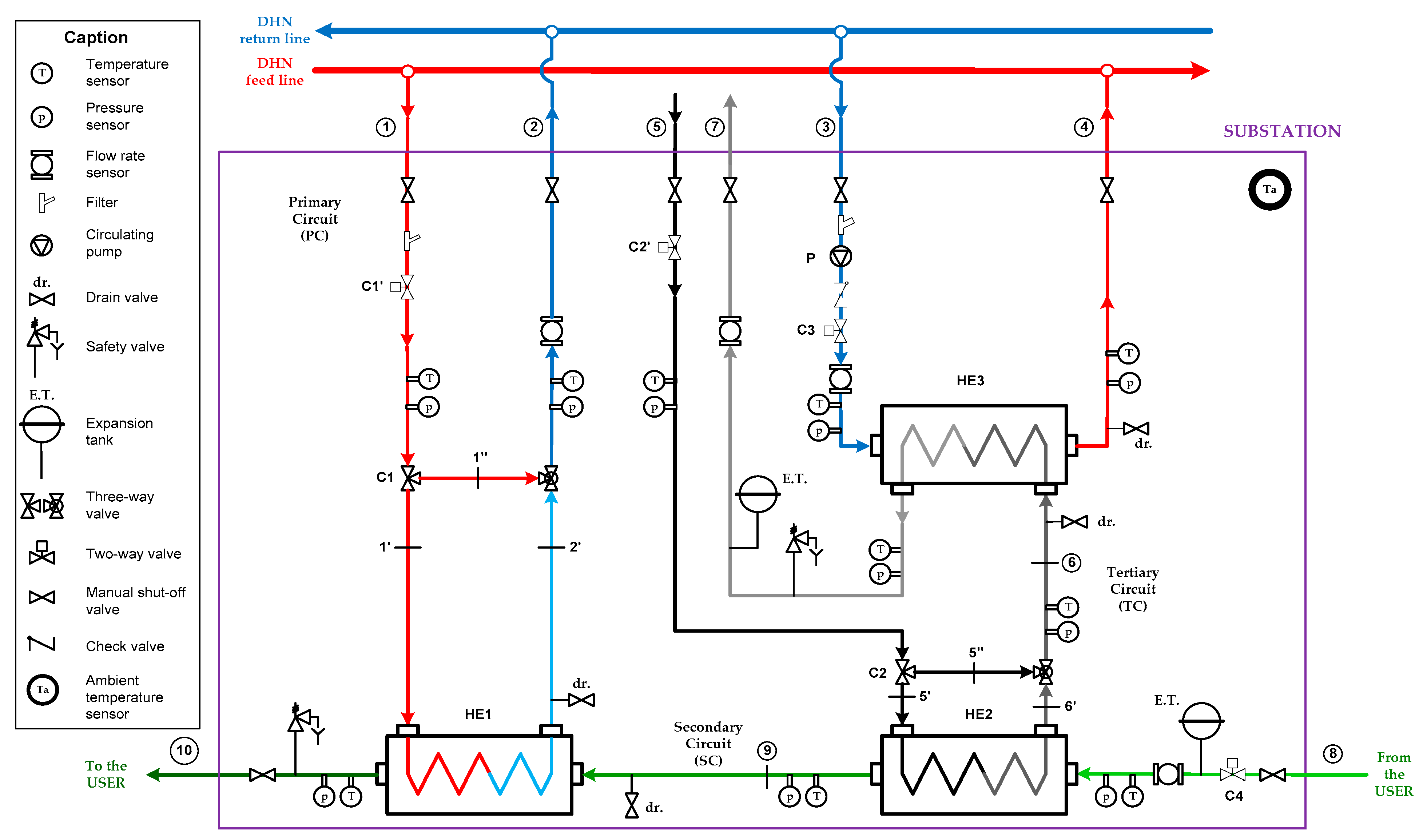
The bidirectional heat exchange substation prototype, conceived by ENEA and UNIBO, was designed to interact with both conventional district heating networks (DHN), and distributed generation systems (e.g., solar thermal panels or heat recovery plants). The prototype is equipped with sensors to monitor and record energy flows, as well as with actuators to control the operation parameters and settings.
Figure 1 shows the layout of the prototype with the installed equipment, including three main circuits connecting the substation to: (i) The supply and the return pipes of the DHN (red and blue, respectively, primary circuit); (ii) The final user (green, secondary circuit); (iii) The distributed generation (DG) system (black and grey, tertiary circuit). The substation is conceived in order to use the heat locally produced to primarily cover the user demand (heat exchanger HE2); in case of surplus, the substation is used to feed the network (HE3). Instead, when there is no local production of heat, the network acts as a heat source (HE1) as in traditional DH.
In detail, the substation is set with a return-to-supply configuration, which means that when the prosumer’s heat production exceeds the user’s demand, then the available thermal energy is used to heat a mass flow rate taken from the return pipeline of the DH up to the temperature value of the supply pipeline, in which the fluid is then re-introduced. This causes a lower mass flow to the power plant and attenuated pressure changes compared to the traditional operation of the network. On the other hand, the heat available from the network is used to fulfill the thermal demand of the user when it cannot be covered by the distributed generation system. The control of substation is temperature- and flow-rate-driven, operated by valves and circulators in the different circuits on the basis of proportional–integral controllers and nominal set values, as summarized in
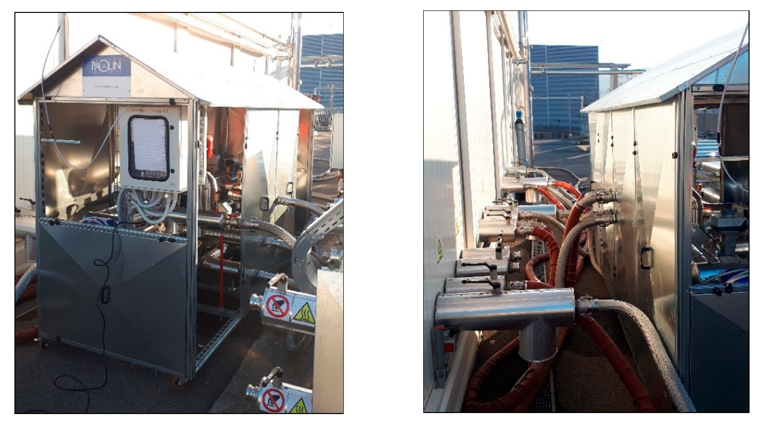
Table 1. The control system briefly includes: 2-way valves C1′, C2′, and C4, meant to keep the flow rate equal to its nominal value on the corresponding circuit; 3-way valves C1 and C2, meant to regulate the hot flow to the HEs based on the target temperature of the fluid leaving the HEs; and a 2-way valve C3, meant to regulate the flow from the DH return to HE3 (C3 is actually fully open because its function is performed by pump P, which can vary its rotation speed). Pictures of the actual installation are included in
Appendix A.
In particular:
Valve C1′ keeps the flow rate M2 constant and equal to its nominal value or excludes HE1 when it is not necessary to achieve the user target temperature T10;
Valve C1 regulates the flow from the DH supply to the HE1 in order to keep the user supply temperature T10 constant; the regulation is operated by redirecting part of the flow to the bypass. In detail: if T10 > T10nom, then C1 redirects the flow bypassing HE1; if T10 < T10nom, then C1 increases the flow rate to HE1; finally, if T10 = T10nom, then C1 maintains the current opening position. Of course, if C1′ is closed, then C1 does not work;
Valve C4 keeps the flow rate M8 constant and equal to its nominal value;
Valve C2′ keeps the flow rate M7 constant and equal to its nominal value or excludes HE2, when the DG return temperature T5 is below the setpoint (user return temperature T8 + ∆T5min), or HE3 when the temperature T5 is below the setpoint (Tmin,DHNfeed);
Valve C2 regulates the flow from the DG to the HE2 in order to keep T9 (outlet temperatures at the secondary side of HE2) equal to the user supply temperature T10; regulation is operated by redirecting part of the flow to the bypass. In detail: if T9 > T10nom, then C2 redirects the flow bypassing HE2; if T9 < T10nom, then C2 increases the flow rate to HE2; finally, if T9 = T10nom, then C2 maintains the current opening position;
Pump P regulates the flow rate M3 from the DH return pipe to the HE3, excluding HE3 when the inlet temperature in the primary side of HE3 (T6) is lower than a minimum value (Tmin,DHNfeed).
More information on the acquisition, monitoring and control systems are included in [
30].
2.2. Modelling
The object-oriented equation-based programming language Modelica and Dymola software were used to optimize the multi-domain simulation and model-based design of dynamic systems as the bidirectional substation. Dymola provides an interactive graphical environment and tools to easily simulate complex system interactions in many fields of engineering, using a mixed symbolic and numerical solver. For the numerical model of the substation, the Modelica, IBPSA and DisHeatLib open-source libraries were analysed, including the relevant classes used in the simulation of the different network components, as summarized below:
Pipes: DynamicPipe (implementing mass, momentum and energy balances, using the energy balance equation); StaticPipe (the model neglects the effect of kinetic energy variations because they are usually not significant compared to heat fluxes, but it includes the potential energy within the energy balance);
Pressure drops: AbruptAdaptor;
Boundary conditions: pressureBoundary_pT (pressure) and MassFlowSource_T (mass flow);
Shut-off valves: ValveDiscrete; the valve provides a small pressure drop proportional to the flow rate if the opening Boolean signal is set to “true”, otherwise the mass flow rate is zero;
Two-way control valves: TwoWayLinear;
Temperature sensors: TemperatureTwoPort;
Pressure sensors: Pressure;
Mass flow sensors: MassFlowRate;
Non-return valves: ValveIncompressible, assuming an incompressible fluid and supporting reverse flow, with a symmetrical flow characteristic curve.
In the sub-section below, the main components modeling is described in detail.
2.2.1. Heat Exchangers
Particular effort was spent in modelling the heat exchangers, as they play a significant role in the bidirectional substation. Since heat exchangers’ behavior is characterized by different dynamics and situations in which each heat exchanger operates in off-design conditions, a new exchanger model at variable efficiency was implemented in Dymola (called
VariableEffectiveness), starting from the one with constant efficiency within the IBPSA’s Fluid library. It inherits the same classes as the exchanger
ConstantEffectivness, but it is able to vary its efficiency depending on the flow rates and on the inlet/outlet temperatures of the fluids (for the hot side T
hot,in and T
hot,out; for the cold side T
cold,in and T
cold,out). According to the thermal resistance scaling method for the evaluation of the heat exchange efficiency during simulations [
31], the total thermal resistance of the heat exchanger at design conditions (
RTD [°C/kW]) is calculated as:
where (
UA)
D is the overall heat transfer coefficient [kW/°C], calculated on the basis of: (i) The convective heat transfer coefficients of the hot and cold fluid α
h and α
c [W/K]; (ii) The thermal conductivity λ of the exchanger material [W/mK]; and (iii) The thickness of the slab [m]. The total thermal resistance value is composed of three contributions, i.e., convection (hot and cold sides) and conduction thermal resistances, taking into account the corresponding factors f
hs (0.46), f
cs (0.46) and f
C (0.13). The thermal resistances at off-design conditions are instead quantified as follows:
where
ṁhs and
ṁcs are the mass flow rates, respectively, of the hot and cold fluid, while subscripts D and OD refer to the design and off-design conditions, respectively.
The total thermal resistance at off-design conditions, the overall heat transfer coefficient, the number of transport units (NTU) and the efficiency ε can, therefore, be calculated as follows:
where
Cmin,OD and
Cmax,OD are, respectively, the minimum and maximum thermal capacities per time unit in off-design conditions. Finally, the design effectiveness is quantified by the following equation:
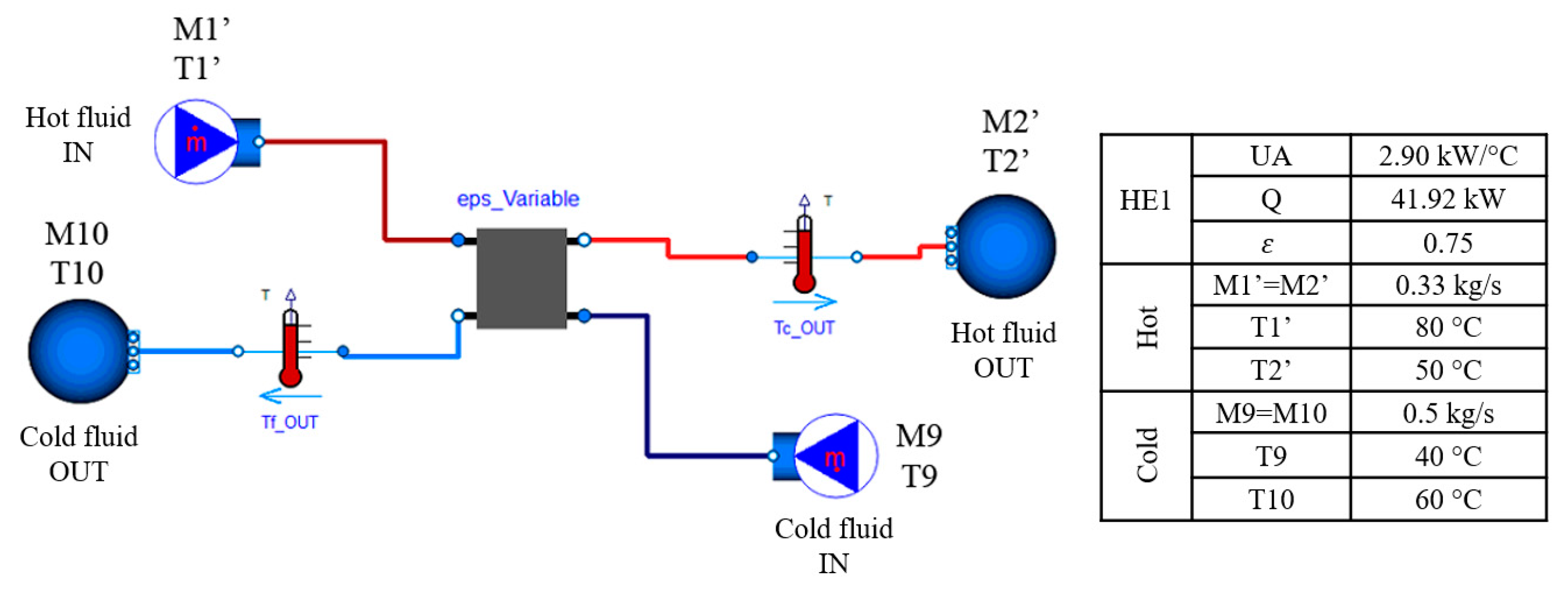
The
VariableEffectivness HE model implements the abovementioned method, and it was used to perform numerical simulations at design and off-design conditions. A simplified layout of HE1 including the heat exchanger and the boundary conditions is shown in
Figure 2.
2.2.2. PID Controllers
As it is well known, a purely proportional controller (P) causes an error proportional correction related to the proportionality constant K. As K increases, the system’s response speed improves and the P outlet value tends to its reference (without reaching it, due to the error at steady-state); on the other hand, oscillations around the set value increase until the system becomes unstable. The integral controller (I) provides a contribution proportional to the integral of the error (i.e., proportional to its mean value) and it removes the steady-state error caused by proportional block. Here, the variable term to be defined is the integration time constant T
i; the smaller the T
i, the greater the integration effect will be, as well as the oscillations that require time before stabilizing. The combination of integral and proportional action (PI controller) ensures greater accuracy, stability of the system and a good speed of response; they are used to obtain a low steady-state error in systems with slow load variations. For the development of the substation model, PI controllers were modelled with
Modelica.LimPID from the
Modelica.Blocks.Continuous.LimPID package, taking into account the integral wind-up problem by suspending the integral action as soon as the output of the controller reaches the saturation level of the actuator [
32].
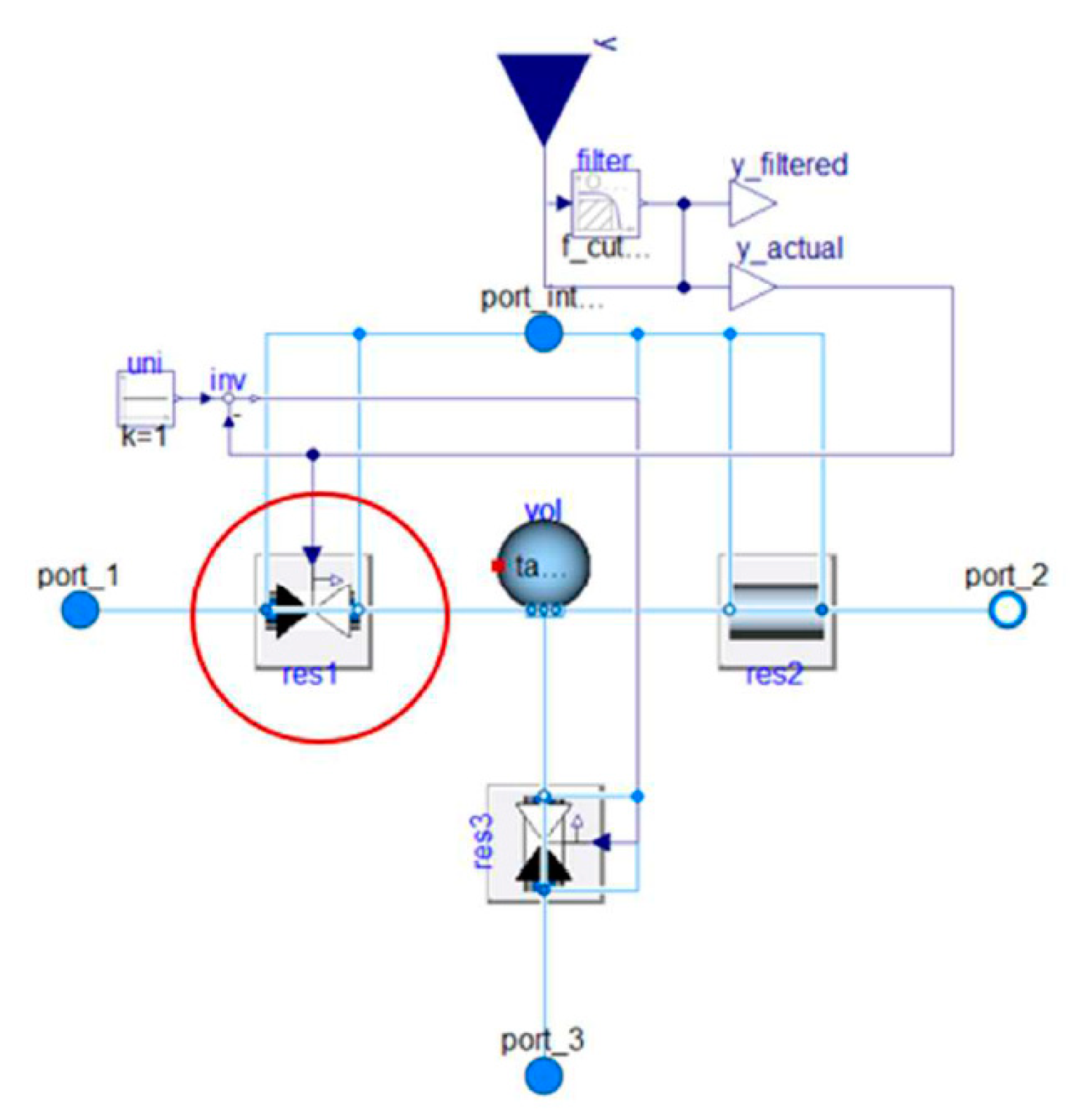
2.2.3. Three-Way Valves
The three-way valve in the substation model is intended to regulate the flow rate at the inlet of the heat exchanger in order to keep the supply temperature to the user constant. This regulation is carried out by the PI controller, which will cause variations in the opening of the valve until the set-point temperature is reached. These valves were modelled by the linear valve component
ThreeWayValveLinear from the IBPSA library, which uses a two-way valve with a linear opening on both main branches (res1 and res3 in
Figure 3) and a pipe with no pressure drop and no transport delay on the by-pass branch. This component is applied to a model characterised by discrete or fast changes in boundary conditions; thus, it is important to pay attention to the implementation of the filter inherited from the
ActuatorSignal class, used to regulate the actuator. It smooths out step changes in the input signal, making the flux continuously differentiable. As a consequence, the controller must be calibrated with the filter within the valve model (this is achieved by setting the parameter
use_inputFilter as “true”, for a second order low pass filter with a “riseTime” of 120 s for a 99.6% closing).
2.2.4. Substation
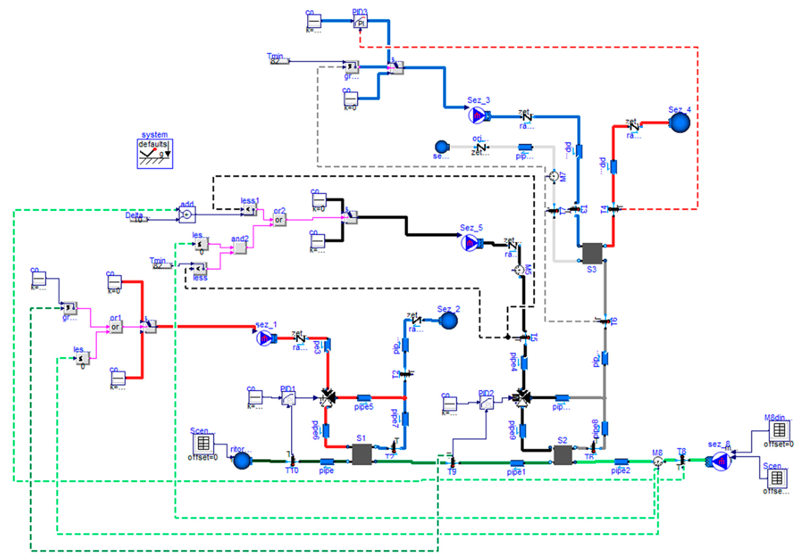
The substation model developed in Dymola is shown in
Figure 4 (dotted lines represent the control signals), edited according to the substation layout in
Figure 1. In addition, the main components are summarized in
Appendix B. As described in
Section 2.1 and in [
30], the model includes the implementation of the control systems: PID1, PI controller acting on the 3-way valve C1 regulating the flow rate from DH supply to HE1; PID2, PI controller acting on the 3-way valve C2 regulating the flow rate from DG to HE2; controls of valves C1′, C2′, C3 and pump P were modelled by acting directly on the boundary conditions, as described below. For these control blocks, a switch component was used resulting in different outputs (u1and u2), depending on the Boolean signal. In detail, Control Block 1, acting as C1′, regulates the interaction with the DHN supply, excluding any flow if the DG covers the user demand (T9 > 59.5 °C, with a tolerance of 0.5 °C from the nominal value) or in case of no demand (M8 = 0); Control Block 2, acting as C2′, regulates the interaction with the DG, setting M5 = M5
nom if T5 ≥ T8 + T5
min, otherwise M5 = 0, and excluding any heat exchange in HE2 and HE3 in case of low DG (T5 < 82 °C) or no demand (M8 = 0); Control Block 3, acting as C3 and P, regulates the interaction with the DHN return, activating the PID3 if T6 > T
min,DHNfeed (82 °C), and thus, controlling the flow rate M3 to maintain T4 at its set point (80 °C), otherwise M3 = 0 and HE3 are switched off. Unlike PID1 and PID2, PID3 was modelled with
IBPSA.LimPid from the IBPSA library because it includes the reverse action option, necessary for a correct control of flow rate M3, depending on the DHN supply temperature T4.
Specific modifications have been applied to the model and its components in order to perform the dynamic simulations described in the following section and presented as results. In particular, conditional blocks were defined in the VariableEffectivness HE model to avoid numerical errors in the case of no flow rate (i.e., efficiency depends on thermal resistance, having the flow rate in off-design conditions as its denominator). The StaticPipe component was selected to replace the DynamicPipe, originally used for stationary tests: indeed, in case of step-varying boundary conditions (as set for dynamic tests), the continuity of the variables is not guaranteed, and the partial derivative balance equations could not be solved; this modification can be avoided with gradual variations in flow rates, expected when coupling the substation to a network model.
As for the limitations of the model, the component selected for the PI controllers (i.e.,
Modelica.LimPID) does not code any hysteresis loop. Analyses performed on the model show that this condition did not cause numerical problems; in case of oscillations around the calibration value, warning alerts or simulation errors, a hysteresis scheme (2 °C) is recommended in order to avoid the intermittent on and off switching of HEs, and thus, to improve their interaction. Finally, the model in
Figure 4 does not include the two expansion vessels, filters, security and drainage valves, as they do not significantly affect the thermo-fluid dynamics.
2.3. Simulations: Analyzed Scenarios and Optimization
The experimental campaign, planned by ENEA and performed by Eurac Research at its energy exchange laboratory in Bolzano (Italy), was aimed at testing the substation under controlled operating conditions and to evaluate the HEs performance and the effectiveness of the implemented control logics in stationary (session A) and dynamic (session B) conditions. In detail, session A included 1-hour tests corresponding to the following scenarios:
Scenario 1: User demand covered by DHN (HE1 active), in design/minimum demand/maximum demand conditions;
Scenario 2: User demand covered by DG (HE2 active) in design conditions;
Scenario 3: DG system supplying the user and DHN (HE2 and HE3 active), minimum user demand;
Scenario 4: User demand covered by DG and DHN (HE2 and HE1 active), maximum user demand;
Scenario 5: DG system feeding DHN (HE3 active), no user demand.
Session B, instead, focused on dynamic conditions, occurring from a stationary state to another. A total of 8 scenarios have been identified and tested, considering different interactions between the substation, the DHN and the DG. These tests (5 ÷ 7 h each) aimed at evaluating how the control logics implemented on the substation respond to the variable conditions in terms of user demand and the generation system production profile, depending on the flow rate M8 and/or the return temperature T8, as well as on the flow rate M5, respectively. T4 and T10 are regulated by PI controllers, while M1, T1, T3 and T5 are constant in each test.
These scenarios were previously experimentally tested on the substation [
30], showing the correct implementation of the control logics and a good performance of the prototype, which always guarantees the satisfaction of the user demand from DG and/or DHN, complying with the requirements for feeding the DG surplus energy into the DHN.
A significant amount of experimental data from all these real-scale tests was used in this work to validate the numerical model of the substation described above. In this study, 3 tests were selected as representatives of the different operating conditions for the substation. In detail:
Test #1: the user demand is covered by DHN (interval length 18,000 s); HE2 and HE3 are not active; HE1 is active for minimum, maximum and nominal user demand (T8 set equal to 50 °C, 30 °C and 40 °C, respectively). T5 from DG is set equal to 35 °C in order to for it to always be lower than temperature T8, which is increased by the minimum temperature difference necessary for the heat exchange (10 °C), thus letting Control Block 2 inactivate HE2 and HE3.
Test #2: the DG covers the user demand and feeds the DHN (interval length 25,200 s); HE1 is not active; HE2 and HE3 are active for different levels of user demand, i.e., maximum, nominal and no demand.
Test #3: the user demand is covered by DG and DHN, and DG also feeds the DHN (interval length 18,000 s); HEs are active for different levels of user heat demand, depending on the M8 dynamic variation.
3. Results and Discussion
In order to investigate the reliability of the
VariableEffectivness HE model, numerical analyses were carried out for each HE of the substation, varying the inlet flow rate on the primary side of HE1, M1′ (0.1 ÷ 0.48 kg/s), and T9 (30 ÷ 55 °C) in six configurations, while T10, M9 and T1′ were kept at design value. Design and off-design results were compared and reported here just for HE1, showing a good match between the two datasets in terms of outlet temperature on the primary side of HE1 T2′ (percentage error between numerical results and analytical values in the range between −0.25% and 0.16%), power Q (−3.70% ÷ 1.67%), heat transfer coefficient UA (−1.71% ÷ 1.30%) and efficiency ε (−5.75% ÷ 1.61%) (
Table 2).
Focusing on the substation model, comparisons between experimental and numerical results are carried out in terms of temperatures, flow rates and thermal power exchange. Regardless of test conditions, the dynamic variations in flow rate and temperature show transient periods in the experimental data, not in the numerical results; this is due to the StaticPipe component, which, unlike the DynamicPipe, solves the mass, energy and momentum balance equations in stationary form. As for the variables T9, T10 and T4 (outlet temperatures at the secondary side of HE2, HE1, and HE3, respectively), the considerable fluctuations in the experimental data during the start-up of the HEs are due to the heating/cooling process of the fluid at the secondary side when the exchanger is inactive; the numerical results do not show the same situation because in the Dymola component, the thermal power zeros when the exchanger is inactive or if there is no flow rate. Due to these considerations, no detailed punctual quantifications in terms of the relative difference between numerical and experimental data are implemented since this analysis is expected to be not significant in this case. Conversely, for each performed analysis, comparisons in terms of the total exchanged thermal energy are implemented.
Results from the 3 representative tests are described and discussed below. For a better comprehension, the prefix EXP (i.e., experimental) is added to the test results and the curves are represented with a thinner line than the one of those based on the numerical simulations.
3.1. Dynamic Analysis #1
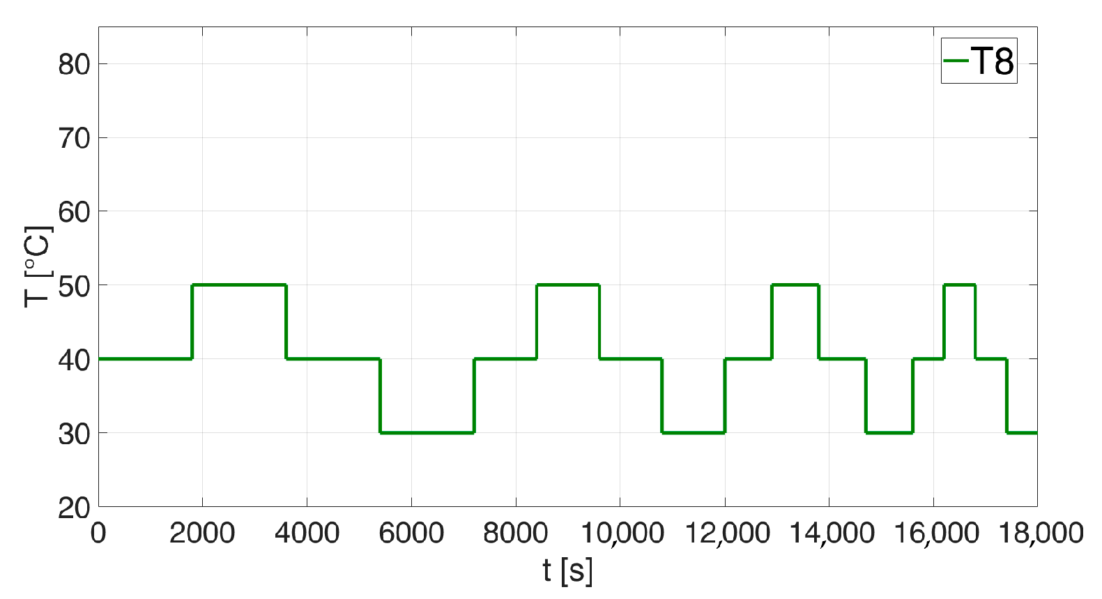
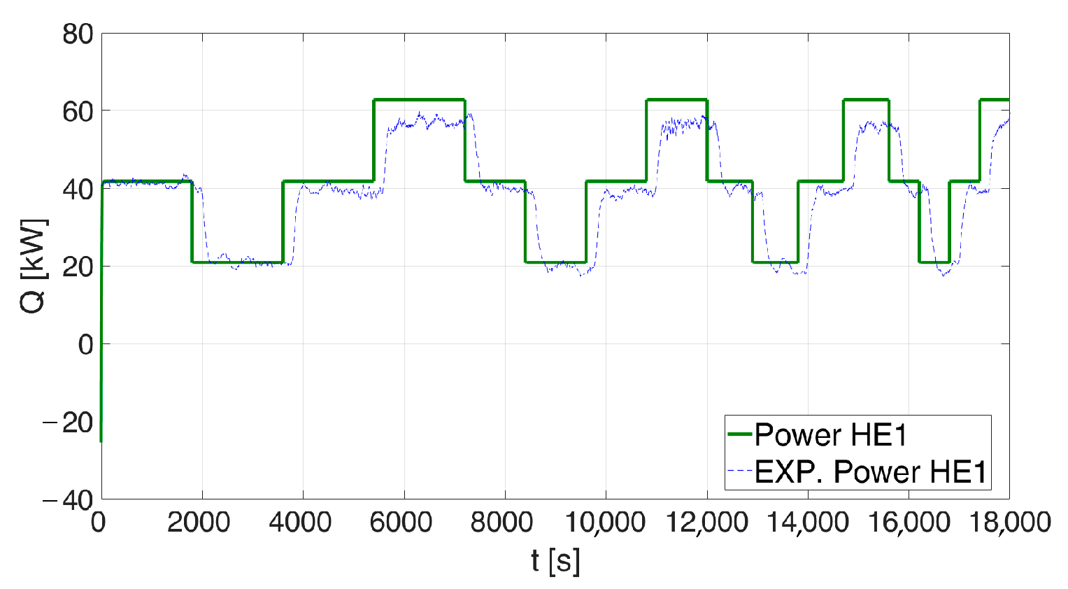
Dynamic Analysis #1 focusses on the operation of the HE1 exchanger (district heating users) for the different levels of thermal demand of the user (minimum, maximum and design demand).
Figure 5 and
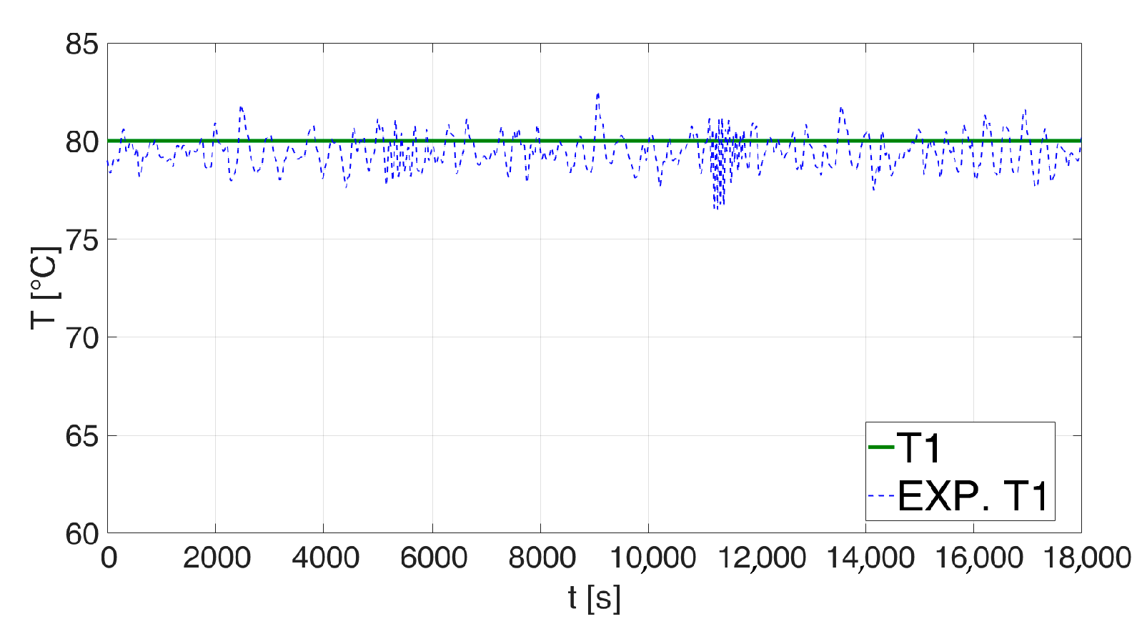
Figure 6 show, respectively, the trend of T8 (user return temperature) and T1 (DHN supply temperature). The T1 set in the numerical model remains constant throughout the simulation, as expected, while the T1 experimentally obtained is characterized by an oscillatory trend, due to the temperature control of the test plant. However, the absolute mean deviation assessed over the entire test remains contained in +/−1 °C.
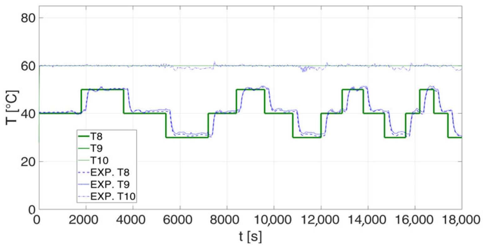
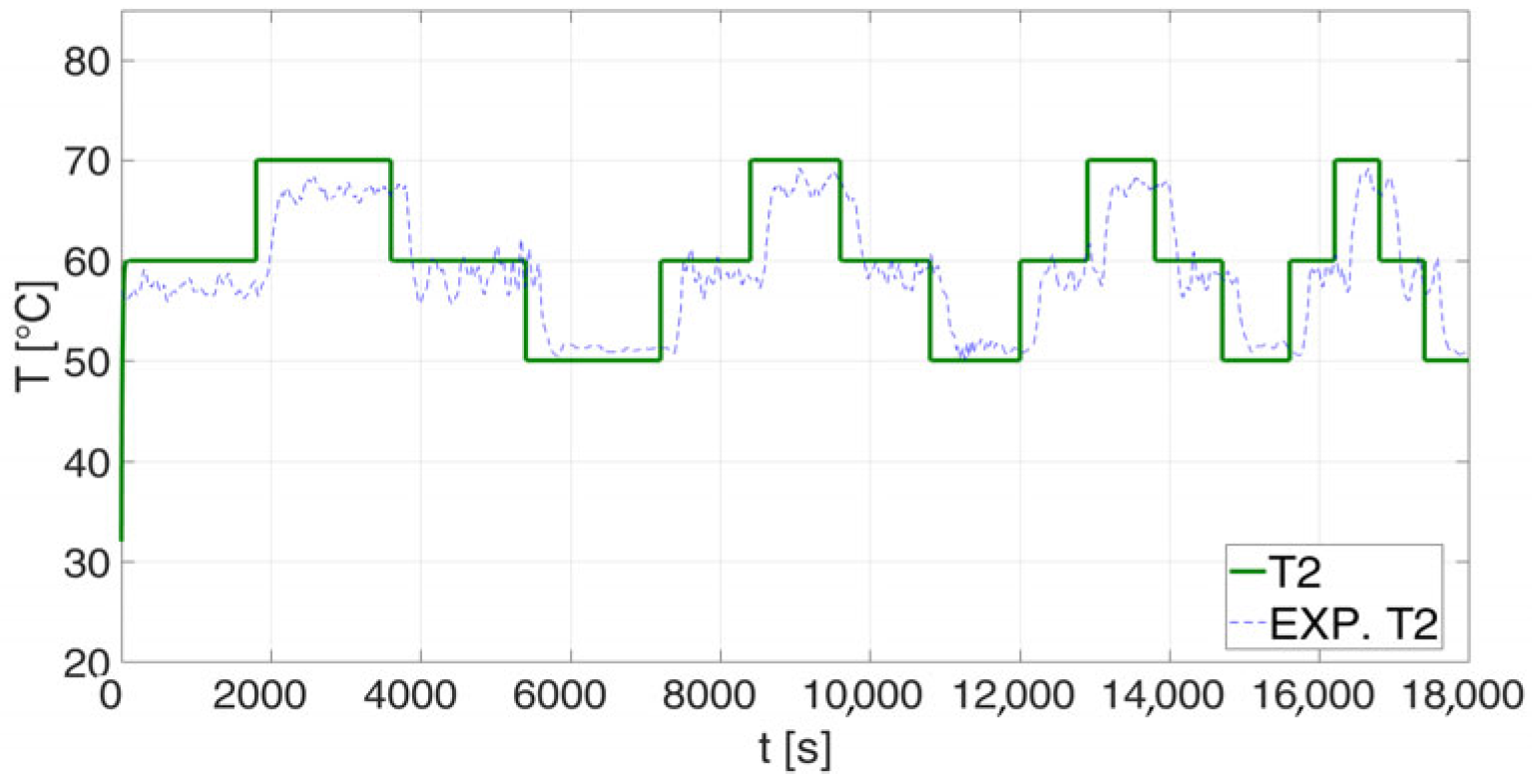
Figure 7 shows the trend of the temperatures from and to the user, i.e., T8, T9 and T10. Since the HE2 is inactive, T8 and T9 obtained from the numerical model perfectly overlap, as expected. It can be noted that the experimental trend of T8 lags behind the one calculated numerically, due to the circuit distance between the test facility point where T8 is controlled and the point in the substation where T8 is measured. However, the absolute mean deviation estimated over the entire test is contained in +/−1 °C. Regarding T10, the discrepancy is less than +/−0.5 °C for most of the test, and the greatest discrepancy is recorded for the maximum request from the user (T8 = 30 °C), representing the limit operating condition for HE1; due to the oscillations in T1 and the thermal losses, it is not possible to obtain exactly 60 °C in T10.
Figure 8 and
Figure 9 show, respectively, the trend of the temperature T2 deriving from mixing flows at T1 and T2′, and the thermal power supplied to the user by the district heating network (HE1). From the comparison, temperature T2 shows a slight delay in the experimental results due the dynamic variation of the boundary conditions T8. As regards the thermal power, HE1 supplied 20.92 kW, 41.84 kW and 62.76 kW for minimum, maximum and design user demand, respectively; it can be noted that a slight delay (a few minutes) of the experimental data exists, which is the result of the delay measured on the T8 temperature. Nevertheless, the maximum relative difference between the experimental result and the numerical outcome in terms of thermal power is less than 15%. When the total thermal energy exchanged by HE1 is analyzed, it is observed that the relative difference between the experimental (194.4 kWh) and the numerical (209.1 kWh) data is very limited and equal to about 7.6%.
3.2. Dynamic Analysis #2
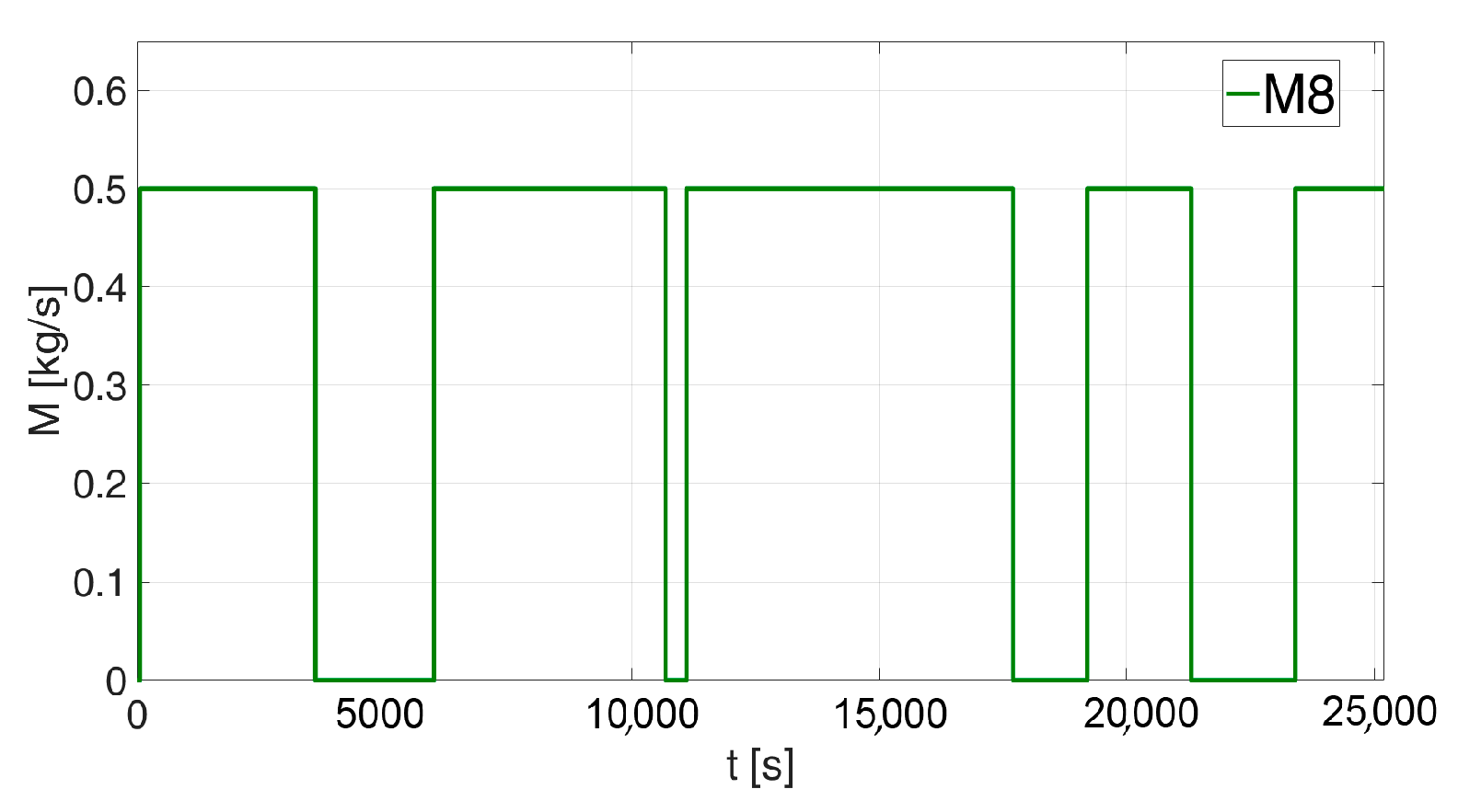
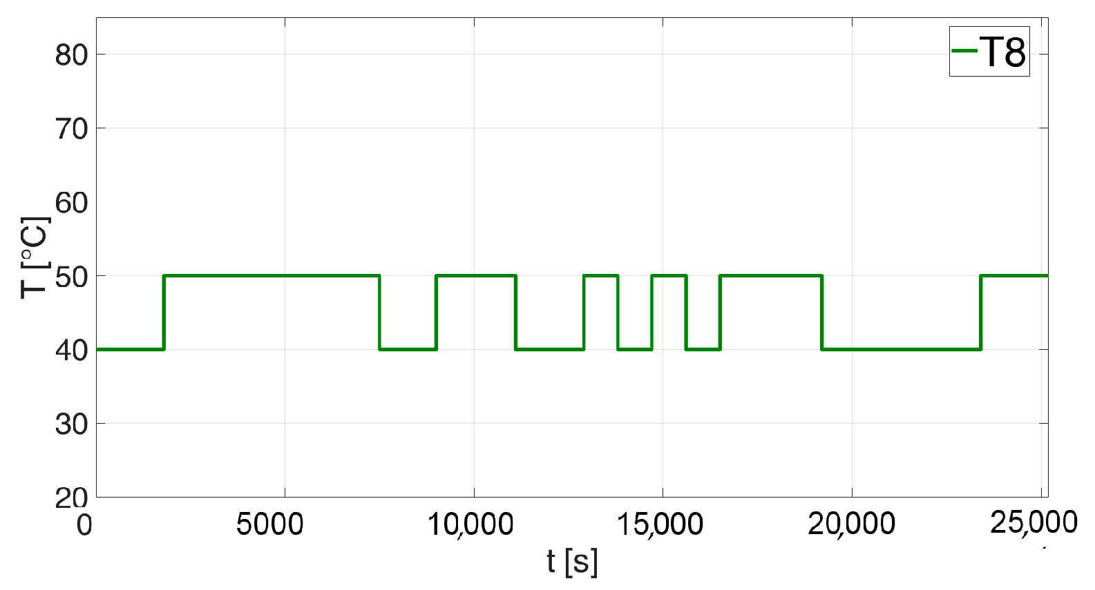
Dynamic Analysis 2 is designed to analyze the operation of the HE2 (distributed generation system) and HE3 (district heating system) exchangers for different levels of user heat demand: design condition, maximum and no demand.
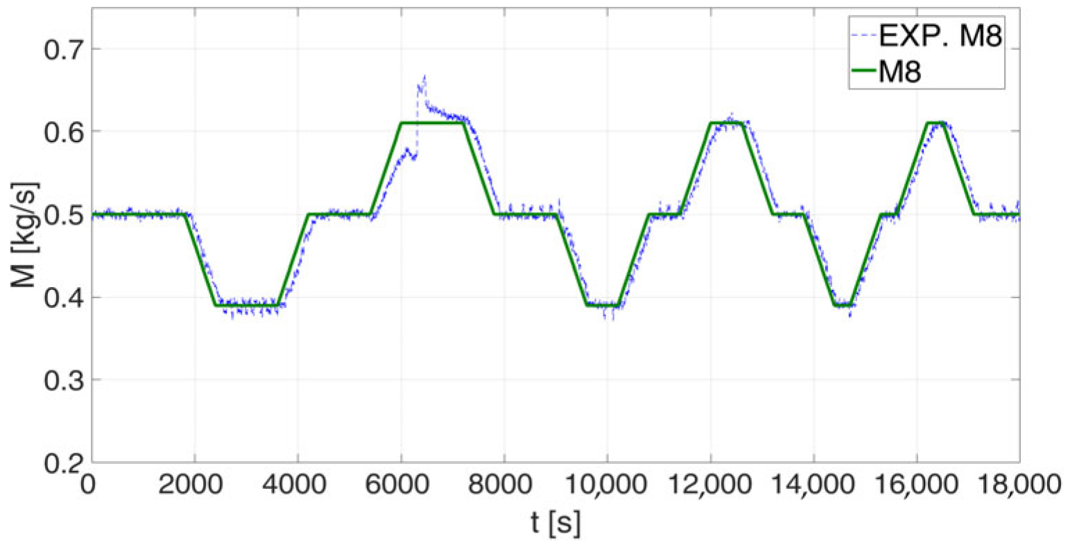
Figure 10 and
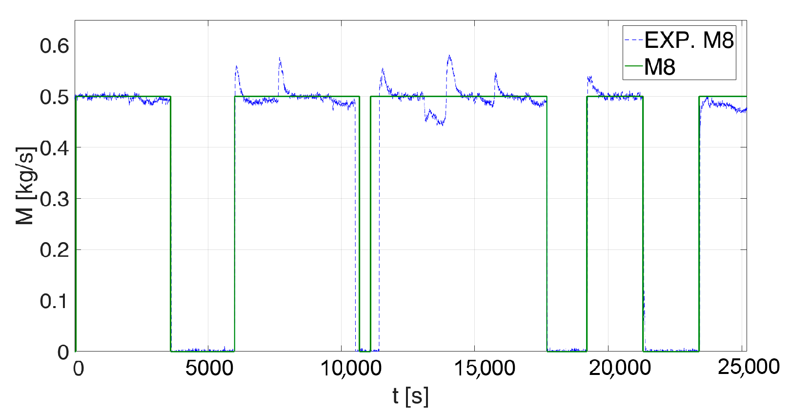
Figure 11, respectively, show the trend of M8 (user flow rate) and T8 (user return temperature); the dynamic variation of these parameters defines the possible cases of the user demand that will be investigated.
Figure 12 shows sudden peaks in the trend of the measured value M8 due to the effects caused on the test plant by the start-ups and shutdowns of the various exchangers in the substation. When these transients are negligible, the maximum absolute difference between numerical and experimental results in terms of M8 is lower than 0.2 kg/s.
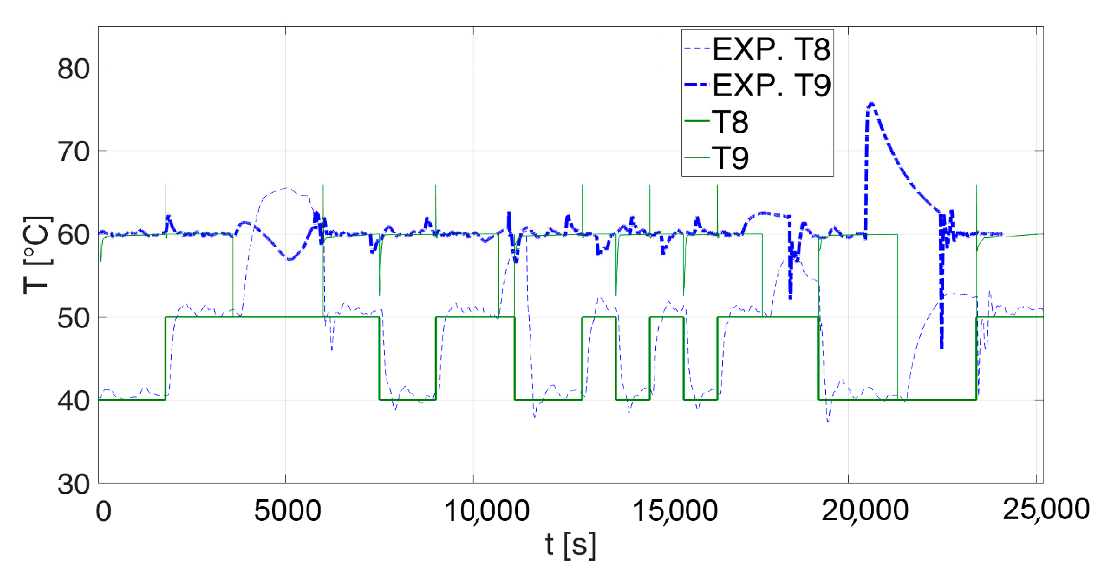
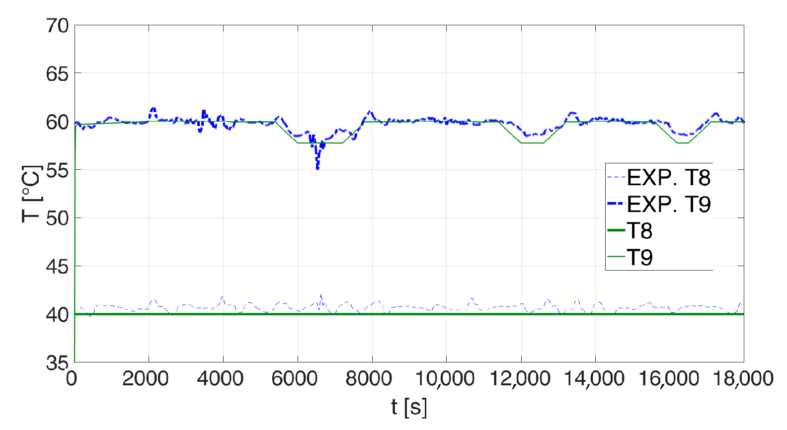
Figure 13 includes the trend of the temperature T8, set as a dynamic boundary condition for the user and of the temperature T9, regulated by the PID2 controller (reference value 60 °C). It can be noted that if M8 = 0 on the user circuit, temperatures T8 and T9 perfectly overlap. Furthermore, focusing on numerical results, the PID2 controller always manages to maintain temperature T9 at the set point value (60 °C), except for the instants related to the instantaneous step variation of T8, in which T9 reaches a peak of up to 65 °C. However, these peaks are resolved in a few tenths of seconds, and then T9 returns to 60 °C (and then never falls below 59.5 °C). Focusing on the experimental data, the peaks in terms of T9 occur very close in time to those observed in the numerical simulations, but they are much more limited in amplitude because of the more gradual experimental variation of T8.
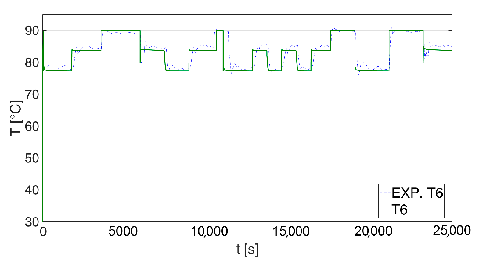
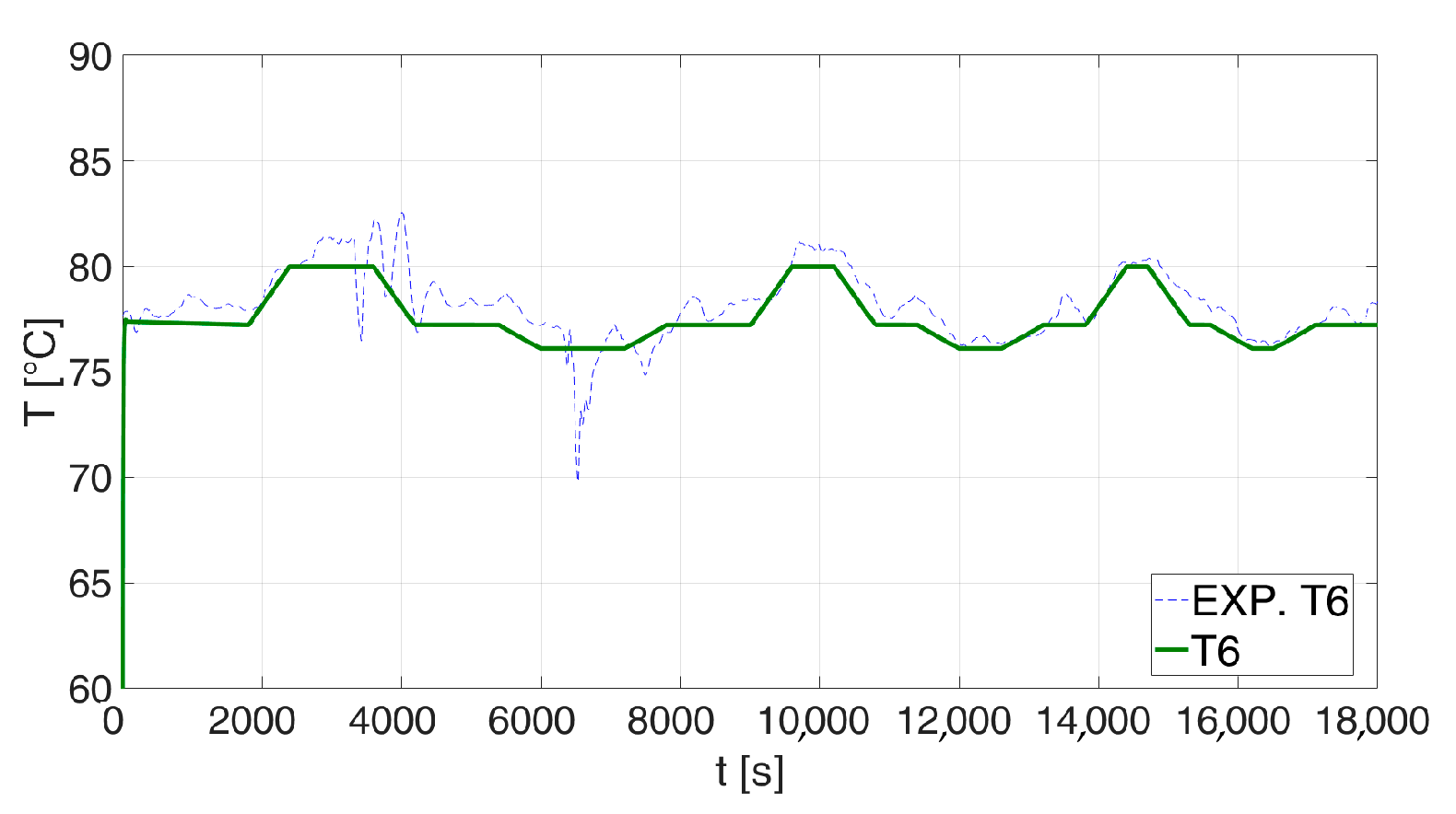
Figure 14 and
Figure 15 show, respectively, the trend of temperature T6 and the flow rates M3 and M7. T6 is the inlet temperature in the primary side of HE3, after mixing the flow coming from the bypass branch of the valve C2 (at temperature T5) and the flow leaving HE2 at temperature T6. Both for temperature and flow rates, the trend of the experimental results is in good agreement with the numerical datasets. In particular, as regards T6 (
Figure 14), when transient effects are negligible, the absolute maximum deviation estimated over the entire test is contained in +/−1 °C. In the case of no user demand (M8 = 0) there is no heat exchange in HE2 and the temperature T6 coincides with T5 (90 °C). Instead, by analyzing
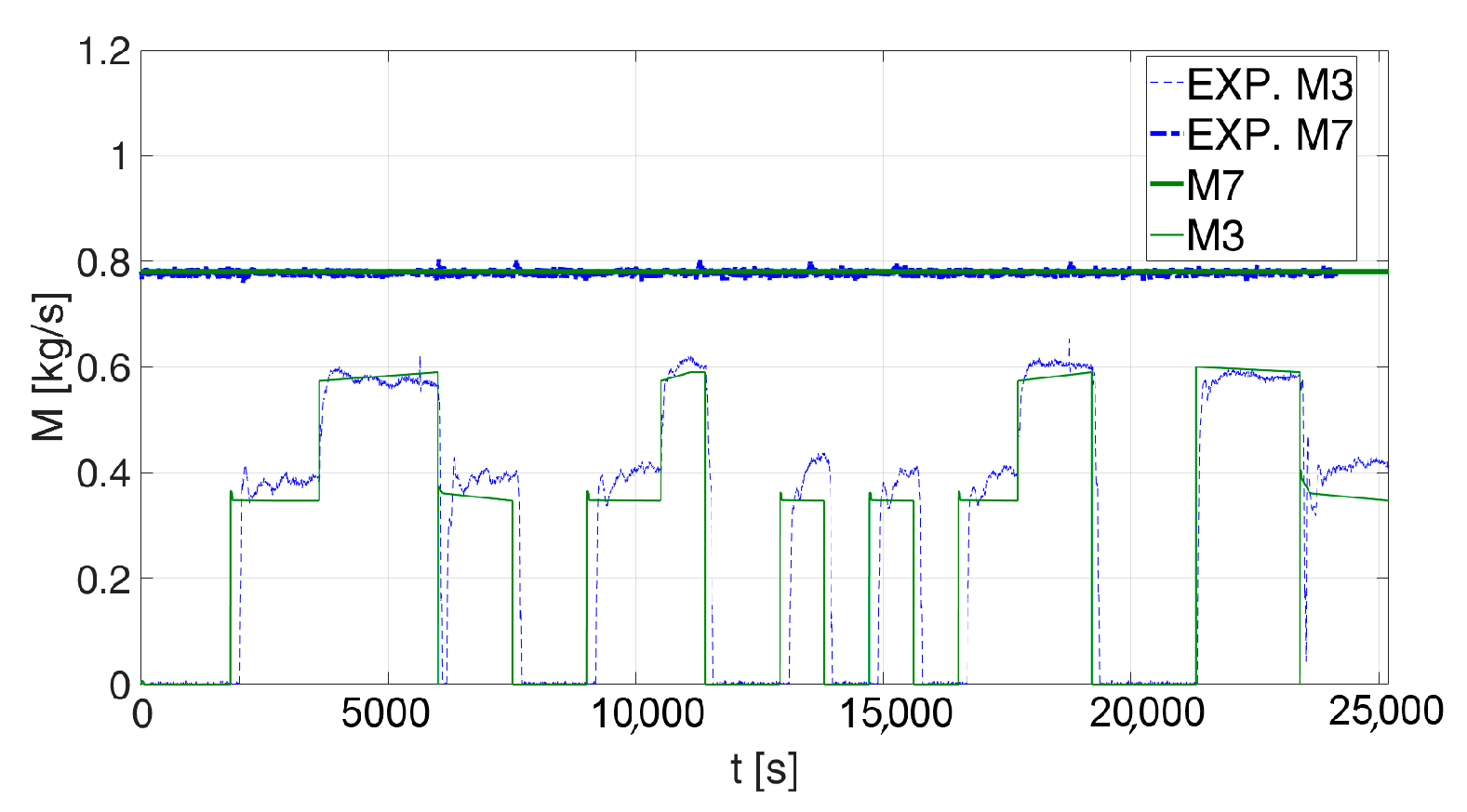
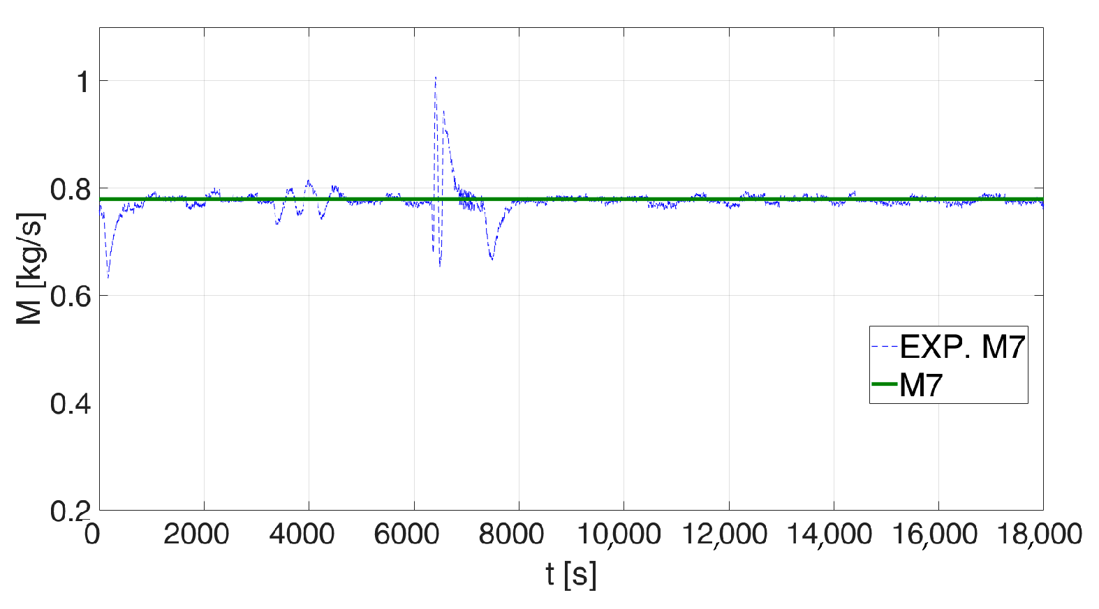
Figure 15 it can be seen that numerical and experimental data in terms of M7 almost overlap entirely, while, in terms of M3, the maximum deviation estimated over the entire test is contained in about 0.09 kg/s.
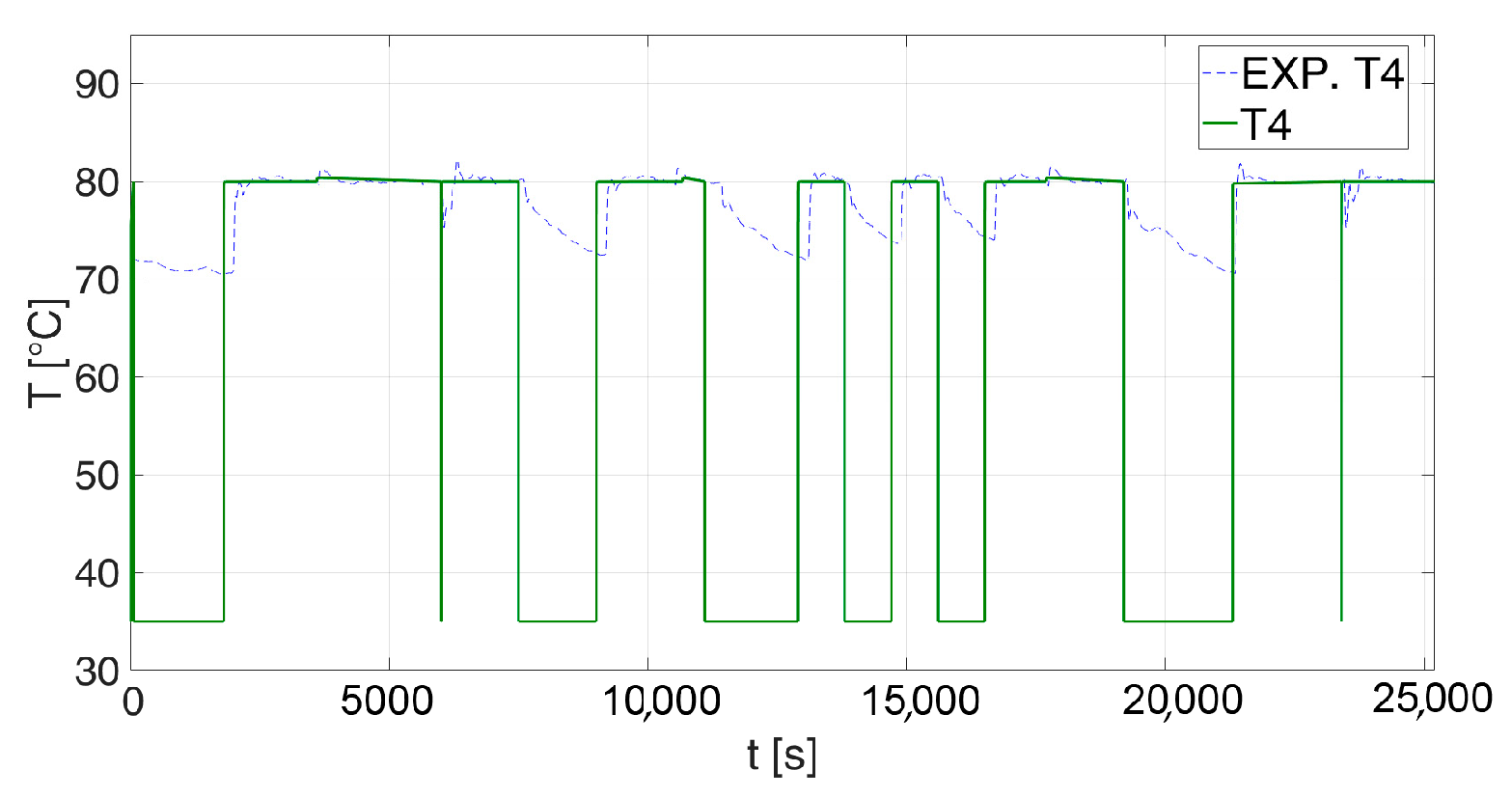
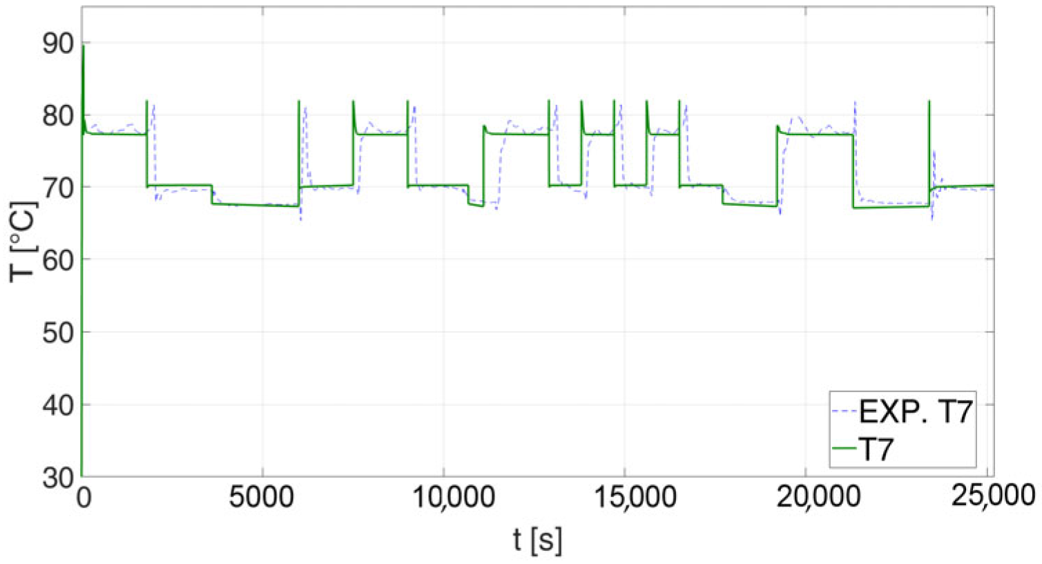
Figure 16 and
Figure 17 show, respectively, the trend of the substation supply temperature to the DHN (targeted at 80 °C) and of the outlet temperature in the primary side of HE3 T7, with a very good agreement between experimental and numerical results (the absolute maximum deviation estimated over the entire test is contained in +/−1 °C for non-zero flow rate M8).
Graphs in
Figure 18 (HE2 exchanger) and
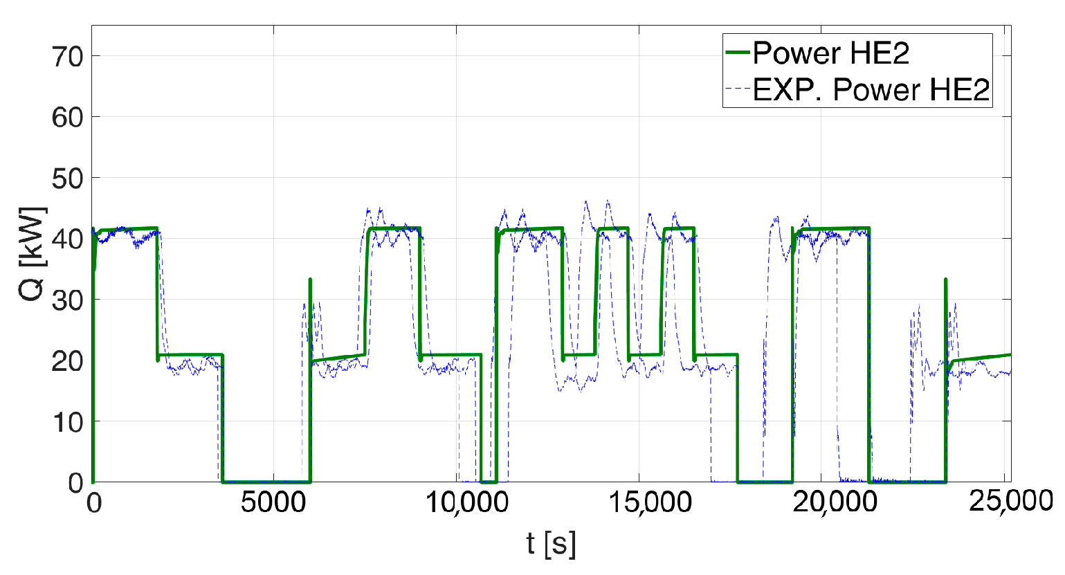
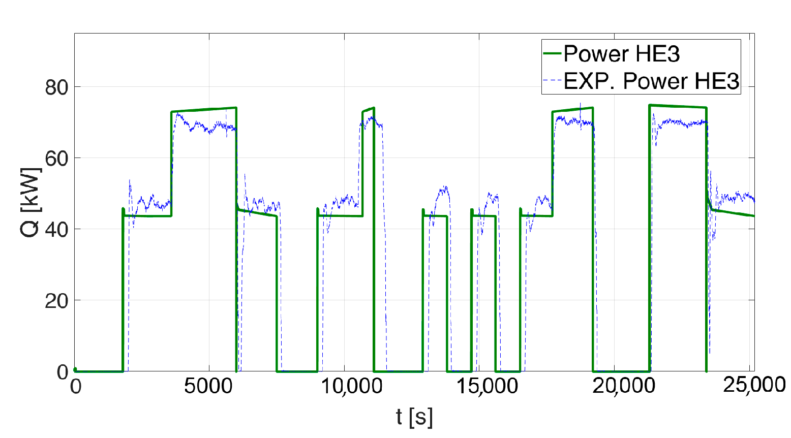
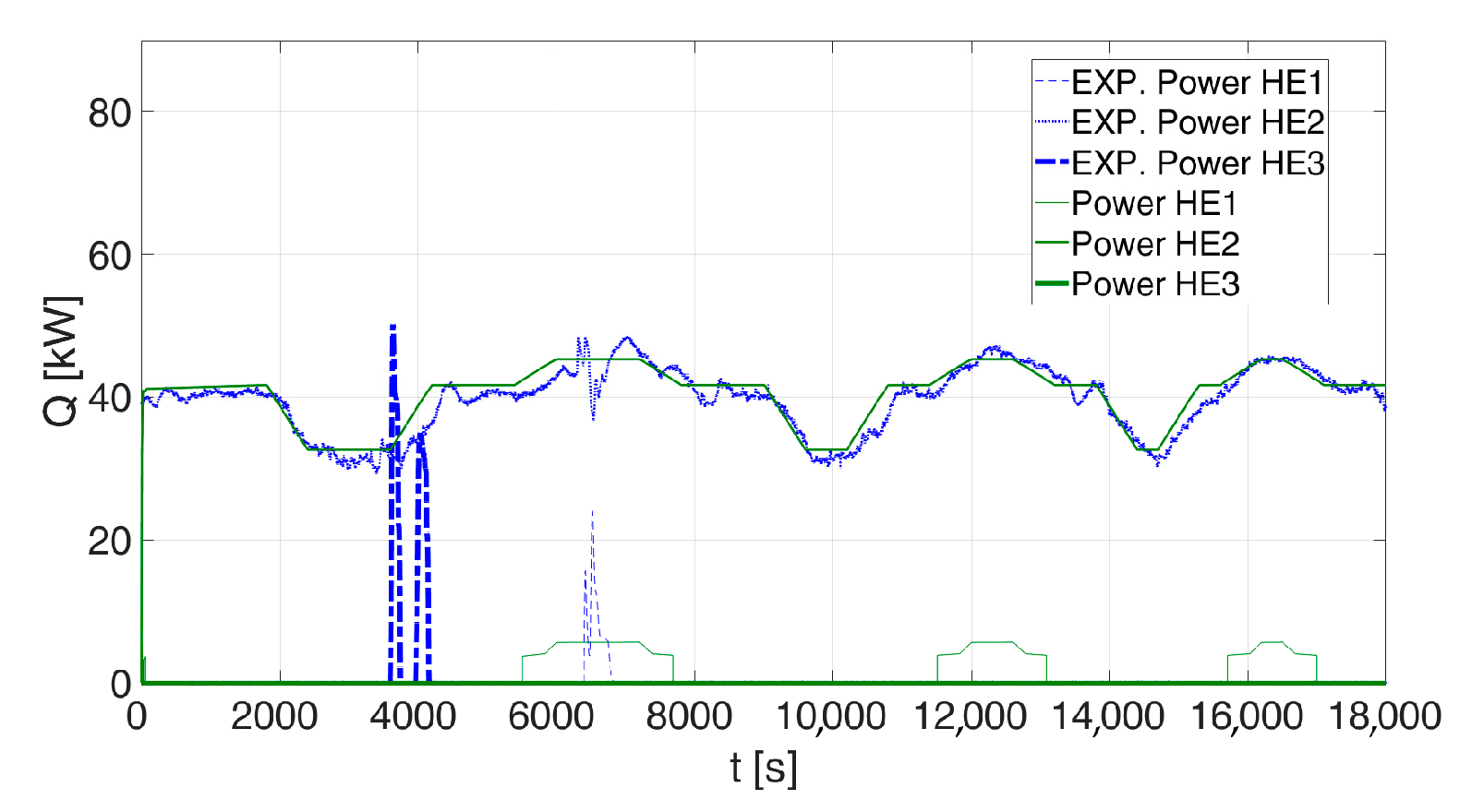
Figure 19 (HE3 exchanger) show how the two exchangers interact. When the thermal power demand is set at design value (about 40 kW), temperature T6 is not sufficient to activate HE3; so, in this case, no thermal energy can be transferred to the DHN. When the thermal power demand is set at the minimum level (about 20 kW) or zero, HE3 is active and part of the DG thermal energy production is used for DHN. The same behavior is observed in the experimental results; in terms of thermal power exchanged by HE2 and HE3, this can be observed numerically as well. The slight differences between the maximum and minimum experimental and numerical values reached by the power exchanged in HE3 is related to the deviation due to the measurement uncertainty of the thermal energy in the primary and secondary circuits. When the total thermal energy exchanged by HE2 is analyzed (
Figure 18), it is observed that the relative difference between the experimental (151.1 kWh) and the numerical (158.7 kWh) data is very limited and equal to about 5.1%. The same comparison regarding HE3 (
Figure 19) is observed to be also very accurate, being the relative difference between the experimental (249.6 kWh) and the numerical (250.6 kWh) data equal to about 0.4%.
3.3. Dynamic Analysis #3
Dynamic Analysis #3 is aimed at analyzing the simultaneous operation of the three HEs for different levels of user heat demand (T8 = 40 °C; M8 variable).
Figure 20 and
Figure 21 show, respectively, the trend of the dynamic variation of M8 (user flow rate) and M7 = M5 (DG system flow rate); a good agreement between experimental and numerical data is obtained for both flow rates (the maximum deviation estimated over the entire test is contained in about 0.1 kg/s, an exception is made for the time instants of HE1 and HE3 activation during the experimental tests).
Figure 22 and
Figure 23 present the trend of temperatures T8, T9 and T6. In detail,
Figure 22 shows how the control system keeps T9 equal to the reference value (60 °C) during the test, except for the time instants in which the flow rate of the user M8 is maximum; in that case, T9 slightly deviates from the set point by a few degrees. Temperature T8, instead, is observed to be constant and equal to 40 °C. Furthermore,
Figure 23 shows the trend of the temperature T6, with a satisfactory agreement between numerical and experimental data. In particular, for T8, T9 and T6, the maximum deviation estimated over the entire test is contained in +/−1 °C, except for the time instants in which HE1 and HE3 activate during the experimental tests.
The thermal powers exchanged in HE1, HE2, and HE3 are shown in
Figure 24. HE3 is activated at the T6 temperature peak after around 1 h (T6 exceeds 82 °C), caused by fluctuations in the T5 temperature control; this oscillation is not observed in the numerical trend, and therefore, HE3 is not active. As for HE1, it is activated when the DG system is unable to reach the T9 reference value (60 °C), a condition that occurs three times, as shown in
Figure 22. In the numerical model, the limit value beyond which there is an exchange with the district heating network is T9 = 59.9 °C; therefore, the HE1 exchanger is activated in all three mentioned periods. On the other hand, in the experimental analysis, the HE1 exchanger is active only in the first period; this behavior might be due to the implementation of a hysteresis loop in the controllers of the substation. As regards the thermal power exchanged by HE2, the maximum relative difference between the experimental result and the numerical outcome is less than 10% (exceptions made for the time instants in which HE1 and HE3 in the experiments activate). When the total thermal energy exchanged by HE2 is analyzed, it is observed that the relative difference between the experimental (198.3 kWh) and the numerical (202.4 kWh) data is very limited and equal to about 2.1%.
3.4. Discussion
Based on the comparison between the results obtained by the application of the developed model and the experimental data, a sufficiently good agreement that enables the validation of the model can be seen. However, further improvements and analyses could be implemented.
As for the developed model, the main limitation stands in the component selected for the PI controllers that does not code any hysteresis loops. This choice does not affect the results presented in this study since the performed analyses on the model show that this condition did not cause numerical problems. However, in the case of oscillations around the calibration value, warning alerts or simulation errors, a hysteresis scheme (2 °C) is recommended in order to avoid the intermittent on and off switching of HEs, and thus, improve their interaction. In addition, the model shown in
Figure 4 does not include some minor components of the prototype, namely two expansion vessels, filters, security and drainage valves, as they do not significantly affect the thermo-fluid dynamics.
As a consequence, in future studies, the authors aim firstly at optimizing the Modelica–Dymola model, and then, at including the optimized model of the bidirectional substation in a complete district heating network model in order to explore the behavior of the substation when integrated with a real network. In particular, the effects of thermal prosumers within the existing traditional DH will be explored, and the possibility of thermal prosumers integration within renewables energy communities will be investigated.
4. Conclusions
In the context of promoting efficient and sustainable energy production and use, this paper is aimed at studying the introduction of thermal prosumers in district heating networks. In particular, a dynamic model of an existing prototype of bidirectional heat exchange substation has been realized, based on the Modelica language and developed with Dymola software. The smart substation has been previously designed by the authors and tested under steady-state and dynamic conditions; consequently, data from experimental campaigns on the real-scale prototype were used in this study to validate the proposed model. Different scenarios, in terms of user demand and heat produced by the distributed generation system at the prosumer site, have been simulated and compared to the experimental data. For Test #1, the mean differences are included in +/−0.5 °C for user supply temperature T10, with increasing discrepancy in the case of maximum user demand (i.e., limit operating condition for HE1, with C1 fully opened). In Test #2, with the dynamic variations of user flow rate and return temperature, controllers effectively operate to maintain set point values in +/−0.5 °C, and resolve instantaneous peaks in a few tenths of a second. In Test #3, the model results in different activations of HEs, overcome the limits of fluctuations in the temperature control during the experimental tests. Transient periods are not included in numerical dataset because of the pipe component used in the model. Furthermore, the fluctuations during the start-up of the HEs are due to the heating/cooling process of the fluid at the secondary side when the exchanger is inactive. Therefore, the main results highlight a generally good agreement between the model and the real operation of the substation.
The results of the Dynamic Analysis made the authors confident about the robustness of the substation model, and a further research activity has been already planned to explore the behavior of the substation when integrated in a complex multi-users network in the framework of the renewable energy communities.


 ,
, 


