Assessment of Object-Level Flood Impact in an Urbanized Area Considering Operation of Hydraulic Structures

Abstract

Urban flooding has become one of the most common natural hazards threatening people’s lives and assets globally due to climate change and rapid urbanization. Hydraulic structures, e.g., sluicegates and pumping stations, can directly influence flooding processes and should be represented in flood modeling and risk assessment. This study aims to present a robust numerical model by incorporating a hydraulic structure simulation module to accurately predict the highly transient flood hydrodynamics interrupted by the operation of hydraulic structures to support object-level risk assessment. Source-term and flux-term coupling approaches are applied and implemented to represent different types of hydraulic structures in the model. For hydraulic structures such as a sluicegate, the flux-term coupling approach may lead to more accurate results, as indicated by the calculated values of NSE and RMSE for different test cases. The model is further applied to predict different design flood scenarios with rainfall inputs created using Intensity-Duration-Frequency relationships, Chicago Design Storm, and surveyed data. The simulation results are combined with established vehicle instability formulas and depth-damage curves to assess the flood impact on individual objects in an urbanized case study area in Zhejiang Province, China.

1. Introduction

Climate change is recognized as causing more frequent extreme precipitation across the globe [1,2,3]. This may subsequently lead to more severe flooding events that threaten people’s lives and cause dramatic damage to property and infrastructure systems, especially in urban areas [4,5]. For example, a pluvial flood occurred in Beijing, China in July 2012 and caused 79 deaths and US $1.86 billion of economic loss [6]. Recently, Zhengzhou, another mega city in China, was hit by severe flooding induced by an extreme rainfall event in July 2021, which affected more than 14 million people and 89,000 homes, and directly caused an economic loss of RMB 114.27 billion [7]. Flash flooding following intense rainfall hit the state of North Rhine-Westphalia, Germany in 2021, leading to 180 deaths and over €12 billion of direct economic loss [8]. The risk of such devastating floods is expected to continue to increase due to climate change and urbanization [9]. It is crucial and urgent to develop more effective flood risk mitigation strategies to save people’s lives and protect their property. The optimized operation of hydraulic structures (e.g., sluicegates, dams and pumping stations) may provide an effective means to support urban flood risk mitigation and management [10,11].

In flood modeling, it has been reported that different representations of sluicegates and other hydraulic structures may significantly affect the predicted results of flood propagation [12,13,14]. Attempts have been made to represent hydraulic structures in hydrodynamic flood models by solving 2D shallow water equations (SWEs) [15,16]. Ratia et al. [17] introduced extra head loss to represent the existence of bridges in a 2D SWE model. Maranzoni et al. [18] presented an approach based on the Preissmann slot concept to simulate pressurized flows through hydraulic structures such as bridges and culverts in a 2D flood model. Most of these approaches are considered to be oversimplified and unable to capture the interactive flow dynamics interrupted by the hydraulic structures as they occur in the real world [19]. Angeloudis et al. [20] developed a source-term coupling approach for modeling sluicegates by directly estimating and including the unit discharge passing through the hydraulic structures in a 2D SWE model. The source-term coupling approach can be easily implemented in a 2D hydrodynamic model, and has been widely adopted by commercial software such as Infoworks Integrated Catchment Modeling (ICM) [21], Environmental Fluid Dynamics Code (EFDC) [22] and Hydrologic Engineering Center’s River Analysis System (HEC-RAS) [23]. However, the source-term coupling approach neglects momentum exchange and may produce inaccurate simulation results.

Zhao et al. [24] implemented internal boundary conditions (IBCs) to account for the presence of hydraulic structures. The IBC method can effectively modify flux computation in a 2D unsteady flow model, and has been adopted by different flood modeling software, such as the open TELEMAC-MASCARET system (TELEMAC-2D) [25] and MIKE 21 [26]. Morales-Hernández et al. [27] modified the IBC method to consider both mass and momentum exchange through flux-term coupling when modelling 2D unsteady flow through a gate. Nevertheless, most of these hydraulic structure modeling approaches involve the use of a weir formula to estimate flow discharge, which requires excessive model calibration to specify discharge coefficients, and therefore may not be transferable to different study sites [19].

Based on the classic Energy-Momentum (E-M) formulation, Cozzolino et al. [28] introduced new discharge formulas for simulating sluicegates, which may be used to estimate the flow discharge through gates even when calibration data are not available [29]. Cui et al. [30] adopted the E-M formulas to support gate modeling, which were fully coupled to a 2D shock-capturing SWE model through the use of both source and flux-term coupling approaches. Such hydraulic structure simulation approaches may be better suited for real-world applications. However, these simulation methods have not been sufficiently evaluated in real-world settings. In highly complex urban environments, Xing et al. [31] recommended that urban flood simulation should be performed at a resolution finer than 5 m to more accurately represent the urban furniture that predominates flood dynamics. In such a high resolution, hydraulic structures are expected to significantly influence the local flood dynamics and affect the overall simulation results, and should therefore be explicitly considered in the modeling process. However, the operation of hydraulic structures has been rarely considered in the application of 2D hydrodynamic models for urban flood modeling and risk assessment.

The aim of this paper is to develop a new high-resolution modeling framework to systematically investigate the effect of hydraulic structures on flood propagation in highly urbanized areas, which is then further exploited to support assessment of flood induced exposure and impact on the individual objects. The rest of the paper is organized as follows: Section 2 introduces the proposed flood modeling framework, including a shock-capturing SWE model, the new approach for direct simulation of hydraulic structures, and finally methods for assessing flood impacts; the study area and datasets are then introduced in Section 3; Section 4 presents and discuss the simulation results; and brief conclusions are drawn in Section 5.

2. Materials and Methods

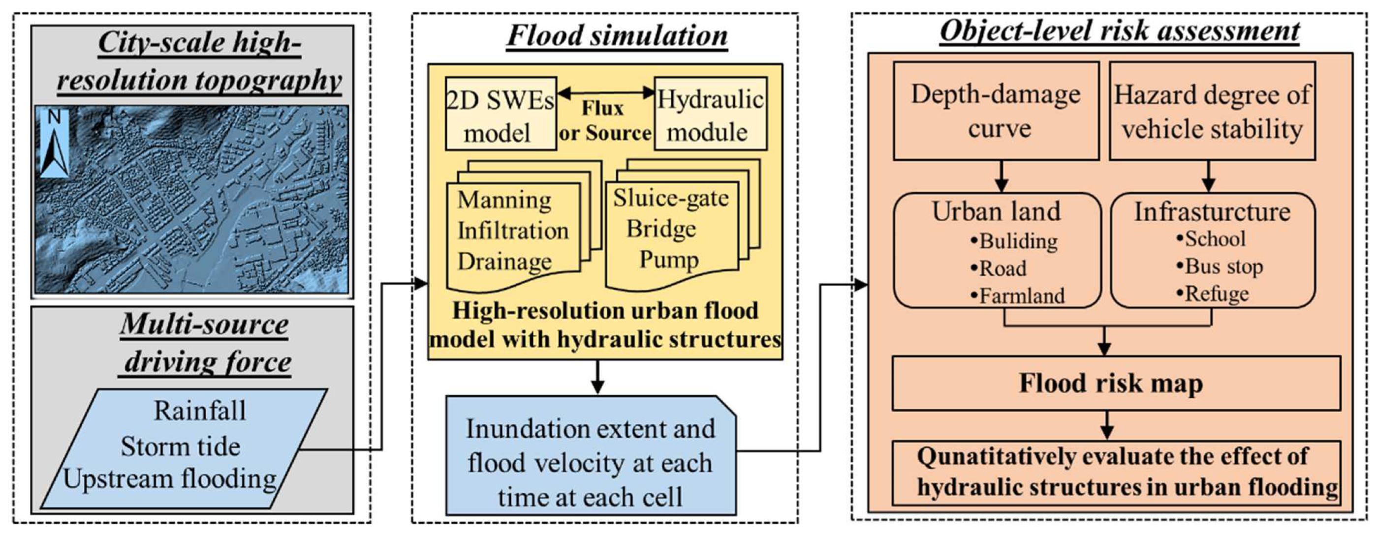
Figure 1 illustrates the proposed numerical framework to consider the operation of hydraulic structures for modeling flood dynamics and assessing object-level flood impact in urban areas. The core of the proposed framework is the new high-resolution urban flood model that includes a hydraulic structure simulation module to predict the highly transient flood hydrodynamics influenced by the operation of hydraulic structures. In this new framework, the highly complex urban topographic features and river networks are represented using the high-resolution digital elevation model (DEM), land-use map and river cross-section data. Driven by rainfall, upstream flow and tidal or surge level as boundary conditions, the model is able to predict multi-source flooding processes interacting with hydraulic structures. The spatially distributed simulation results, including flow depth and velocity, can be then overlaid with the spatial data detailing the types and locations of different objects to pinpoint their exposure to flooding. Established depth-damage curves and vehicle instability formulas are further adopted to assess the flood impact on individual objects. The respective components of this flood modeling and impacted assessment framework will be explained in more detail in the following sub-sections.

2.1. The 2D SWE Model

A fully 2D hydrodynamic flood model generally solves the nonlinear SWEs, which can be written in a matrix form as [32]

$$\frac{\partial \mathbf{q}}{\partial t}+\frac{\partial \mathbf{f}}{\partial x}+\frac{\partial \mathbf{g}}{\partial y}=\mathbf{S}$$

(1)

where t, x, and y are the time and Cartesian coordinates, respectively; q denotes the vector containing the flow variables; f and g are the flux vectors in the x- and y-directions; and S is the source term vector. The vector terms may be given by

$$\begin{gathered} \mathbf{q}=\left[\begin{array}{c}\eta \\ q_x^{\ast }\\ q_y^{\ast }\end{array}\right],\mathbf{f}=\left[\begin{array}{c}{q}_x^{\ast }\\ u^{\ast }{q}_x^{\ast }+g\left({\eta }^{\ast }{}^2-2{\eta }^{\ast }{z}_b\right)/2\\ u^{\ast }vh\end{array}\right] \\ \mathbf{g}=\left[\begin{array}{c}{q}_y^{\ast }\\ v^{\ast }uh\\ v^{\ast }{q}_y^{\ast }+g\left({\eta }^{\ast }{}^2-2{\eta }^{\ast }{z}_b\right)/2\end{array}\right],\mathbf{S}=\left[\begin{array}{c}R+S_{\mathrm{HS}}\\ -g\eta \partial z_b/\partial x-{\tau }_{bx}/\rho \\ -g\eta \partial z_b/\partial y-{\tau }_{by}/\rho \end{array}\right] \end{gathered}$$

(2)

where η represents the water surface elevation above the datum (i.e., water level); u and v are the depth-averaged velocity in the x and y-directions; z_b is the bed elevation above datum; h = η − z_b is the total water depth; R = r − f − s represents surface runoff with r being the rainfall intensity, f being the infiltration rate and s being the drainage loss; g is the gravity acceleration; $-\partial z_b/\partial x$ and $-\partial z_b/\partial y$ give the bed slopes in the two Cartesian directions; ρ is the water density; and τ_bx and τ_by are the friction stresses in the x and y-directions calculated using

$${\tau }_{bx}=\rho C_{f}u\sqrt{u^2+v^2},{\tau }_{by}=\rho C_{f}v\sqrt{u^2+v^2}$$

(3)

where C_f = gn²/h^1/3 is the roughness coefficient, with n being the Manning coefficient.

The types of hydraulic structures considered in this work are categorized into line/polyline and point/polygon structures. Hydraulic structures such as sluicegates, dams, bridges and culverts may be idealized as lines or polylines in a 2D computation domain, which are defined as line/polyline structures in this work. Similarly, hydraulic structures such as pumping stations may be idealized as point/polygon structures. In Equation (2), the flux vectors f and g are modified and a source term S_HS is added to simulate different hydraulic structures directly.

To enable the development of a robust coupling scheme to consider the operation of hydraulic structures in large-scale urban flood modeling, the unit-width discharges in the x and y-directions are redefined as $q_x^{*}$ and $q_y^{*}$, given as follows

$$q_x^{\ast }=\left\{\begin{array}{cc}uh& \mathrm{at}\mathrm{cell}\left(i,j\right)\\ q_{\mathrm{HS}x}& \mathrm{at}\mathrm{cell}\left(i_{\mathrm{HS}},j_{\mathrm{HS}}\right)\end{array}\right.,q_y^{\ast }=\left\{\begin{array}{cc}vh& \mathrm{at}\mathrm{cell}\left(i,j\right)\\ q_{\mathrm{HS}y}& \mathrm{at}\mathrm{cell}\left(i_{\mathrm{HS}},j_{\mathrm{HS}}\right)\end{array}\right.$$

(4)

Similarly, $u^{*}$ and $v^{*}$ are redefined as

$$u^{*}=\left\{\begin{array}{cc}u& \mathrm{at}\mathrm{cell}\left(i,j\right)\\ u_{\mathrm{HS}}& \mathrm{at}\mathrm{cell}\left(i_{\mathrm{HS}},j_{\mathrm{HS}}\right)\end{array}\right.,v^{*}=\left\{\begin{array}{cc}v& \mathrm{at}\mathrm{cell}\left(i,j\right)\\ v_{\mathrm{HS}}& \mathrm{at}\mathrm{cell}\left(i_{\mathrm{HS}},j_{\mathrm{HS}}\right)\end{array}\right.$$

(5)

where (i, j) denotes a normal computational cell whilst (i_HS, j_HS) represents a hydraulic structure cell, $q_{\mathrm{HS}x}$, $q_{\mathrm{HS}y}$, $u_{\mathrm{HS}}$ and $v_{\mathrm{HS}}$ are utilized to represent the flow variables affected by line/polyline hydraulic structures. The effects of point/polygon-type hydraulic structures are considered through the new mass source/sink term, S_HS. These newly introduced flow variables/terms will be further introduced in the following Section 2.2 and Section 2.3.

A Godunov-type finite volume scheme incorporated with an HLLC (i.e., Harten-Lax-van Leer with Contact wave restored) approximate Riemann solver is used to calculate the interface fluxes and solve the above SWEs [33,34,35]. The surface reconstruction method (SRM) and implicit friction discretization scheme are implemented to ensure the stable and accurate simulation of overland flows in urbanized areas [36,37]. To substantially improve the computational efficiency for large-scale, high-resolution simulations, the model has been further implemented on multiple Graphics Processing Units (GPUs) via the NVIDIA CUDA computational platform to achieve high-performance computing [35].

2.2. Hydraulic Module

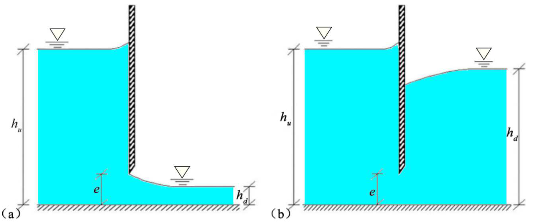
The flow through a line/polyline structure, e.g., a sluicegate, possibly free-surfaced or submerged [38], as illustrated in Figure 2. The discharge of a low flow or an overtopped high flow (i.e., free-surface flow unaffected by the structure) does not require any special treatment, i.e., directly calculating as uh or vh in Equation (2). The unit-width discharge q_HS affected by such a structure may be estimated using a discharge formula. For a sluicegate, an Energy-Momentum (E-M) formula [39] may be used to estimate the discharge, which is considered to be valid even when calibration data is not available [28,29].

For the flow through a sluicegate as shown in Figure 2, assuming a contraction coefficient of ε = 0.611 for both cases, the discharge under the free-flow condition may be calculated by [28]

$$q_{\mathrm{HS}}=\frac{\epsilon }{\sqrt{1+\frac{\epsilon e}{h_u}}}e\sqrt{2g{h}_u}$$

(6)

where h_u is the upstream water depth; h_c = εe is the flow depth at the vena contraction, with e being the gate opening.

With reference to h_c, the downstream subcritical flow depth h_c^# may be calculated using the Belanger’s equation as

$$h_c^{\#}=\frac{h_c}{2}\left(-1+\sqrt{1+8\frac{q_{\mathrm{HS}}^2}{g{h}_c^3}}\right)$$

(7)

If the downstream depth h_d > h_c^#, the flow is submerged and the discharge is then estimated by

$$q_{\mathrm{HS}}=\sqrt{\frac{1-\frac{H}{h_u}}{1-\frac{\epsilon e}{h_u}}}\frac{\epsilon }{\sqrt{1+\frac{\epsilon e}{h_u}}}e\sqrt{2g{h}_u}$$

(8)

with

$$H=h_u\left[\frac{2\left(\frac{h_u}{\epsilon e}-\frac{h_u}{h_d}\right)}{{\left(\frac{h_u}{\epsilon e}\right)}^2-1}+\sqrt{{\left(\frac{2\left(\frac{h_u}{\epsilon e}-\frac{h_u}{h_d}\right)}{{\left(\frac{h_u}{\epsilon e}\right)}^2-1}-1\right)}^2+{\left(\frac{h_d}{h_u}\right)}^2-1}\right]$$

(9)

For other types of line/polyline structures, the discharge formula may need to be adapted according to the structure type. For example, bridges and culverts are common types of hydraulic structures in urban cities and pressurized flow may develop when the water height rises to the low chord of the bridge or culvert. Under such a flow condition, the following discharge formula may be used [40]

$$q_{\mathrm{HS}}=C_d\sqrt{2g\left(H_0-\frac{Z}{2}\right)}$$

(10)

where the discharge coefficient C_d = 0.5 is commonly used in practice; H₀ is the total head upstream; and Z is the water depth from the low chord to the bed level z_b.

For point/polygon structures such as pumping stations, the flow discharge is determined according to the corresponding pumping capacity (e.g., maximum design discharge) and operation practice.

2.3. Coupling Approach

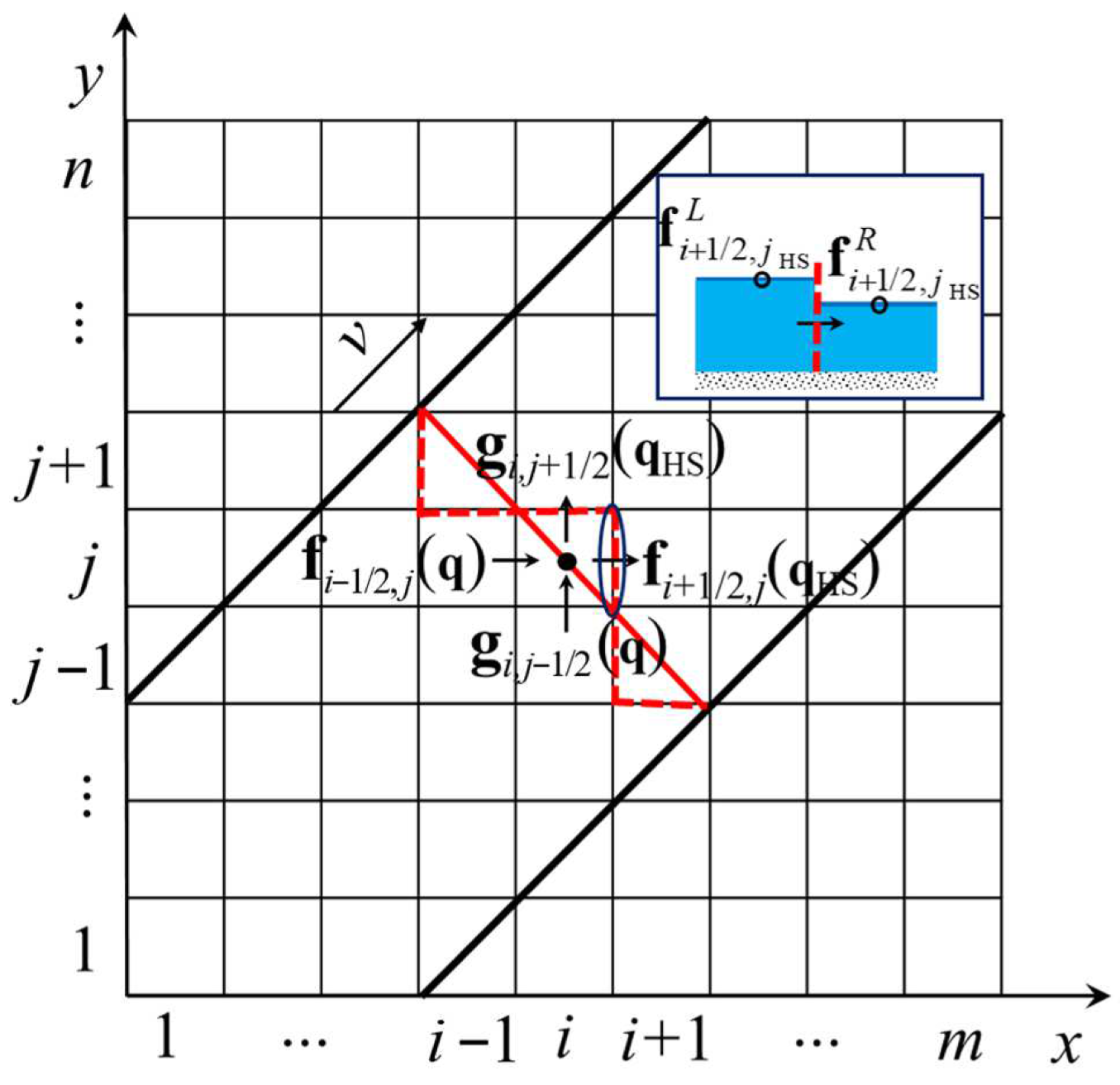
The flux-term and source-term coupling approaches [30] are both considered in this study to couple the hydraulic structure calculation module to the 2D SWE model. A flux-term coupling approach [24,27] was adopted to directly simulate the effect of a line/polyline hydraulic structure in the 2D SWE model. As shown in Figure 3, the two bold black lines are used to define a channel reach. The line/polyline hydraulic structure indicated by the red solid line is approximated by the red dotted lines in a stairs-case manner on the 2D computational grid. The cell edges that overlap with the red dotted lines are HS cell edges, and a cell containing a HS cell edge is regarded as a HS cell, differentiating from the normal cells and normal cell edges.

In a finite volume scheme, as adopted in this study, the flow variables q at HS cell (i, j) as shown in Figure 3 may be updated to a new time level as

$${\mathbf{q}}_{{\mathrm{HS}}_{i,j}}^{k+1}={\mathbf{q}}_{{\mathrm{HS}}_{i,j}}{}^k-\frac{\Delta t}{\Delta x}({\mathbf{f}}_{i+1/2,j}({\mathbf{q}}_{\mathrm{HS}})-{\mathbf{f}}_{i-1/2,j}(\mathbf{q}))-\frac{\Delta t}{\Delta y}({\mathbf{g}}_{i,j+1/2}({\mathbf{q}}_{\mathrm{HS}})-{\mathbf{g}}_{i,j-1/2}(\mathbf{q}))+\Delta t{\mathbf{S}}_{i,j}^k$$

(11)

where the superscript k is the time level, Δx and Δy represent the cell size in the x and y-directions; Δt is the time step; f_i+1/2,j (q_HS) and g_i,j+1/2 (q_HS) respectively denote the fluxes at the east and north cell edges of HS cell (i, j). Whilst the HLLC approximate Riemann solver is used to calculate the fluxes across a normal cell edge, the flux calculation at the left and right sides of the HS cell edge i + 1/2 is modified as:

• Under the free flow condition

  $${\mathbf{f}}_{i+1/2,j}^u=\left[\begin{array}{c}{q}_{\mathrm{HS}}\\ \frac{q_{\mathrm{HS}}^2}{h_{i,j}}+\frac{g}{2}\left({\eta }_{i,j}^2-2{\eta }_{i,j}{z}_{b_{i,j}}\right)\\ \frac{q_{\mathrm{HS}}}{h_{i,j}}vh\end{array}\right],{\mathbf{f}}_{i+1/2,j}^d=\left[\begin{array}{c}{q}_{\mathrm{HS}}\\ \frac{q_{\mathrm{HS}}^2}{h_c}+\frac{g}{2}\left({\eta }_c^2-2{\eta }_c{z}_{b_c}\right)\\ \frac{q_{\mathrm{HS}}}{h_c}vh\end{array}\right]$$

  (12)
• Under submerged flow condition

  $${\mathbf{f}}_{i+1/2,j}^u=\left[\begin{array}{c}{q}_{\mathrm{HS}}\\ \frac{q_{\mathrm{HS}}^2}{h_{i,j}}+\frac{g}{2}\left({\eta }_{i,j}^2-2{\eta }_{i,j}{z}_{b_{i,j}}\right)\\ \frac{q_{\mathrm{HS}}}{h_{i,j}}vh\end{array}\right],{\mathbf{f}}_{i+1/2,j}^d=\left[\begin{array}{c}{q}_{\mathrm{HS}}\\ \frac{q_{\mathrm{HS}}^2}{h_c}+\frac{g}{2}\left({\eta }_H^2-2{\eta }_H{z}_{b_H}\right)\\ \frac{q_{\mathrm{HS}}}{h_c}vh\end{array}\right]$$

  (13)
• Under partially pressurized flow

  $${\mathbf{f}}_{i+1/2,j}^u=\left[\begin{array}{c}{q}_{\mathrm{HS}}\\ \frac{q_{\mathrm{HS}}^2}{h_{i,j}}+\frac{g}{2}\left({\eta }_{i,j}^2-2{\eta }_{i,j}{z}_{b_{i,j}}\right)\\ \frac{q_{\mathrm{HS}}}{h_{i,j}}vh\end{array}\right],{\mathbf{f}}_{i+1/2,j}^d=\left[\begin{array}{c}{q}_{\mathrm{HS}}\\ \frac{q_{\mathrm{HS}}^2}{h_{i+1,j}}+\frac{g}{2}\left({\eta }_{i+1,j}^2-2{\eta }_{i+1,j}{z}_{b_{i+1,j}}\right)\\ \frac{q_{\mathrm{HS}}}{h_{i+1,j}}vh\end{array}\right]$$

  (14)

  where the unit-width discharge q_HS is calculated using Equations (6)–(10), depending on the flow conditions. The y-direction HS fluxes can be obtained similarly.

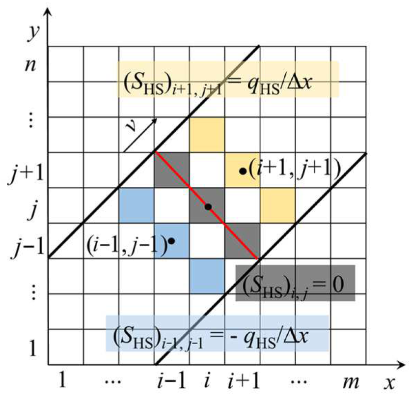
The source-term coupling approach [20] is applied to evaluate the effect of a point/polygon hydraulic structure. As shown in Figure 4, the location of point/polygon hydraulic structures inside the channel is indicated by the red solid line, with source cells ‘receiving’ mass flow marked in blue and the sink cells ‘providing’ mass flow marked in orange. The cells defining the hydraulic structure (marked in grey) allow zero flux to get through. The associated source/sink term is then calculated through

$$S_{\mathrm{HS}}=\left\{\begin{array}{c}-q_{\mathrm{HS}}/\Delta x\\ q_{\mathrm{HS}}/\Delta x\end{array}\right.\begin{array}{c}\mathrm{at}\mathrm{the}\mathrm{source}\mathrm{cell}\\ \mathrm{at}\mathrm{the}\mathrm{sink}\mathrm{cell}\end{array}$$

(15)

2.4. Flood Hazard and Risk Assessment

This framework assesses the flood hazard degrees of vehicles to critical infrastructures such as schools, bus stations and relevant disaster reduction centers. It also assesses the potential damage to individual objects such as buildings, farmlands and roads, which is an important component of flood risk management. In the proposed flood modeling and risk assessment framework, the spatially distributed flood simulation results are overlaid with spatial exposure data detailing the types and locations of different objects, e.g., vehicles, buildings, farmlands, and roads to assess flow impact. For vehicles, the hazard degree (HD) may be estimated using the following vehicle instability criteria [41]:

$$U_c={\alpha }_c{(\frac{d}{h_c})}^{{\beta }_c}\sqrt{2g{l}_c[{\rho }_c{h}_c/(\rho h_f-R_f)]}$$

(16)

$$\mathrm{HD}=\min (1.0,v/U_c)$$

(17)

where U_c represents the incipient velocity for a vehicle; α_c and β_c are empirical coefficients; l_c, b_c and h_c are the length, width and height of the vehicle under consideration; ρ_c is the vehicle density; h_f represents the floating depth and R_f = h_cρ_c/(ρh_k). A vehicle is considered to be safe if HD = 0 and if it will be in danger if HD approaches 1.0.

Flood damage assessment provides important information for flood risk management [42]. As the main land use types related to social economic development [43], buildings, farmlands, and roads are often highly vulnerable to flooding [44,45,46]. To assess flood damage to these objects, the depth-damage curves proposed by Huizinga et al. [47] for buildings, farmlands, and roads (Figure 5a–c) were adopted in this work. These curves have been widely applied in different countries and regions across the world [42,48,49].

3. Case Study

The application of the proposed flood modeling and risk assessment framework involves (1) collecting spatial data, hydro-meteorological data and information of hydraulic structures for model set up, and socio-economic data for risk/impact assessment; (2) simulating flooding process; and (3) overlaying the flood simulation results with spatial exposure data to quantify flood impact/risk. Herein, the Damaiyu Subdistrict of the Yuhuan City, China was selected as the case study to demonstrate the proposed framework for real-world application.

3.1. Study Area

Yuhuan City, China, is located on the southeast coast of Zhejiang province and is also the mid-point of the gold coastline (121° E, 28° N). The Damaiyu Subdistrict in Yuhuan is a highly urbanized area surrounded by mountain ridges except for the south side, which is open to the estuary of Qinglan River (Figure 6a). The study area has a subtropical monsoon climate characterized by an obvious marine climate, receiving an annual average rainfall of 1500 mm (China Meteorological Administration, http://www.cma.gov.cn/, accessed on 26 November 2021). The region is frequently affected by extreme rainfall and cyclonic storms, especially during the flood season (Chinese weather website, http://www.weather.com.cn/, accessed on 25 December 2021). The study site has been frequently hit by severe floods due to its geographic location and climate characteristics, and many of these flood events have a compound nature (http://www.yuhuan.gov.cn/, accessed on 26 November 2021). The local river system is regulated by ten control gates and two tidal gates (Figure 6b). Damaiyu Subdistrict, therefore, provides an ideal case study to investigate the multi-source flooding processes and the impact in a highly urbanized area including operation of hydraulic structures.

3.2. Model Setup

This section describes the key data used to model the flood events, including a high-resolution Digital Elevation Model (DEM), a land use map, and information on hydraulic structures, rainfall and tidal level.

• Digital Elevation Model

The Digital Elevation Model (DEM) is a regular grid structure with a grid resolution of 3 m, which was provided by the Zhejiang Institute of Hydraulics & Estuary. The values of DEM elevation vary from −3.5 to 332.2 m (Figure 6a). Areas labeled as A1~A6 in Figure 6a represent flooding areas (i.e., Chenbei village, Old town, Intersection of Xingzhong Road and Longshan Road, Xinmin community, Shiwumu village and Huanhai village), obtained by survey data.

2.

Land-use patterns

The land use data was extracted by OpenStreetMap (http://download.geofabrik.de/, accessed on 20 January 2021) and sub-meter imagery from ArcGIS Server (http://services.arcgisonline.com/arcgis/services/, accessed on 20 January 2021) includes roads, mountain areas, farmlands, buildings, water bodies and other built-up areas (Figure 6b).

The selection of model parameters, including Manning coefficients, infiltration parameters, and drainage capacity, corresponds to the relevant land use type. The selection of Manning coefficients is based on typical values as suggested by McCuen et al. [50]. The Manning coefficient is valued at 0.02 for roads, 0.08 for mountain areas and farmlands, 0.05 for buildings, 0.035 for rivers and other bare grounds in the high-resolution urban flood model. The parameters of the infiltration rate (i.e., hydraulic conductivity, wetting front metric potential and wetting front depth) for the Green-Ampt model are obtained by Brakensiek and Onstad [51]) and Rawls et al. [52]). The drainage loss is valued at a rate of 13.2 mm/h according to the Code for Design of Outdoor Wastewater Engineering (GB 50014-2021).

3.

Specific information on focused hydraulic structures

The study site has twelve sluicegates, including ten control gates and two tidal gates (Figure 6b). These sluicegates are located in Qinglantang River, Sangutang River, Liurong River, Gushun River and Caopitang River and Waitang River, respectively. Single-hole control gates (Chenyu, Sangutang and Gushun gates in Figure 6b) remain open, while other control gates in Figure 6b are usually closed, except if the upstream water level is higher than the downstream water level. For two tidal gates in Figure 6b, Yongfu and Mitongao gates, lifting them to release flooding when the upstream water level is higher than the water level of the inflow boundary, otherwise, closed them.

4.

Rainfall and tidal level

The rainfall and tidal level define the boundary conditions of the study domain. The boundary conditions drive the simulations to simulate a completely multi-source flood and well consider the urban conditions. More details will be introduced in the following Section 3.3.

In this work, all of the simulations are performed on a server computer equipped with Intel^® Xeon^® E5-2650 v3 processor (two Core, 2.3 GHz, 16 GB DDR4) and NVIDIA Tesla K80 GPU device (two Kepler GK210 GPUs).

3.3. Driving Force Data Availability and Processing

3.3.1. Typhoon Lekima (2019)

The powerful Typhoon Lekima (known as Typhoon Hanna in the Philippines) has led to 45 deaths and caused 45.38 billion Yuan RMB (USD 6.43 billion) of economic loss in Zhejiang province (https://en.wikipedia.org/wiki/Typhoon_Lekima, accessed on 25 December 2021). Figure 7a shows the time history of rainfall and accumulated rainfall recorded in a local rainfall station (Figure 6a). As shown in Figure 7a, Lekima directly brought heavy rainfall of over 200 mm in a few hours. Figure 7b shows the tidal level at the same time period in which the high tide actually coincided with maximum rainfall; the location of the tidal station can be shown in Figure 6a. The surveyed data provided by the Zhejiang Institute of Hydraulics & Estuary indicates that the severe flooding was mainly due to the typhoon-induced intense rainfall, but not the riverbank breaching. However, both the rainfall and tidal level were considered in the numerical model to obtain a better understanding of fully hydrodynamic processes during the event.

3.3.2. Extreme Designed Scenario

As precipitation is the external driving force of urban flooding, the information should be used as an input to flood hazard analysis. Most cities in China have their municipal models of Intensity-Duration-Frequency (IDF) relationships, accounting for local precipitation characteristics [45]. The Yuhuan Municipal Engineering Design Institute develops the Yuhuan rainstorm IDF formula. Rainfall intensities with a duration of one hour and a return period of 20, 50, 100, and 200 years were formulated to cover the probable inundation situations. The formula can be expressed as follows:

$$q=5.543(1+0.862\lg P)/{(t+5.116)}^{0.509}$$

(18)

where q is the rainfall intensity, P is the return period of rainfall, and t is the duration of rainfall.

Chicago Design Storm has been extensively applied in the design storm, as the pattern includes the average intensities of the rate-duration curve for all durations [45,53]. Chicago Design Storm is employed to calculate peak intensity and then redistribute the rainfall before and after the peak with the relevant spectrum of durations [53]. The parameter r (i.e., the ratio of time of the peak to the total) is empirically fixed at 0.4 in Yuhuan City according to the standards for local flooding prevention and control system planning published by the Department of Housing and Rural-Urban Development of Zhejiang Province (http://jst.zj.gov.cn/module/download/downfile.jsp?classid=0&filename=ba64fb090dd840b4a52ea52cb428f27a.pdf, accessed on 20 December 2020). In combination with Yuhuan IDF analysis, it enables the design of rainstorms corresponding to the defined return periods. The generated rainfall fields (Figure 8a) display a spatial uniformity and a 1-min temporal resolution. The equations of the Chicago method can be written as follows:

$$i_a=\frac{a\times \left[\frac{\left(1-c\right)\times t_a}{1-r}+b\right]}{{\left(\frac{t_a}{1-r}+b\right)}^{c+1}}$$

(19)

$$i_b=\frac{a\times \left[\frac{\left(1-c\right)\times t_b}{r}+b\right]}{{\left(\frac{t_b}{r}+b\right)}^{c+1}}$$

(20)

where i_a is the rainfall intensity after the peak (mm/min); i_b is the rainfall intensity before the peak (mm/min); t_a is the time after the peak (min); t_b is the time before the peak (min); a, b and c are the parameters function of the location and the frequency.

At the same time, information on the tidal level at the estuary of the study area should be used as an input to flood hazard analysis. In this work, the maximum surface elevation of Typhoon 9711 (Winnie) (Figure 8b) has been chosen as the time series of tidal levels for the boundary of Qinglan estuary. Typhoon 9711 generated the most significant storm surge (center of wind speed and pressure reaching 60 m/s and 920 hPa) at Haimen Station in Taizhou city since the creation of the People’s Republic of China (PRC). It caused 248 deaths, more than 5000 people were injured, and it caused a direct economic loss of 4.3 billion RMB [54].

4. Results and Discussion

To evaluate the model’s performance, simulated water depths are compared with the observed depths at the gauging points. The Nash-Sutcliffe Efficiency (NSE) coefficient [55] was adopted to quantify the discrepancy between simulated and observed water depth, which is defined as

$$NSE=1-\frac{{{\displaystyle \sum }}_1^N{\left(h_m^n-h_0^n\right)}^2}{{{\displaystyle \sum }}_1^N{\left(h_0^n-\overline{h_0}\right)}^2}$$

(21)

where $h_m^n$ and $h_0^n$ represent the simulated and observed water depth at time step n, respectively; h₀ denotes the mean observed water depth; and N is the total number of time steps. NSE ranges from −ꝏ to 1. NSE = 0 indicates that the model predictions are as accurate as the average of the observed data while NSE = 1 represents a perfect match between observations and predictions. Additionally, a better agreement between the predictions and observations is achieved when the value of NSE is closer to 1.

The Root-Mean-Squared Error (RMSE) is also adopted to assess the accuracy/difference of the simulation results. It is written as:

$$RMSE=\sqrt{\frac{1}{N}{{\displaystyle {\sum }_1^N\left(h_m^n-h_0^n\right)}}^2}$$

(22)

A lower RMSE indicates higher simulation accuracy, and a value of 0 means a perfect fit to the observed/referenced data.

F-statistics was chosen to quantify how well the simulated flood extent matches the observed one. Its expression is shown as follows:

$$F\left(\%\right)=\frac{A-B}{A+B+C}\times 100$$

(23)

where A represents the number of correctly predicted flooded cells, B counts the number of cells erroneously predicted as flooded, and C denotes the number of cells erroneously predicted as dry.

4.1. Model Validation

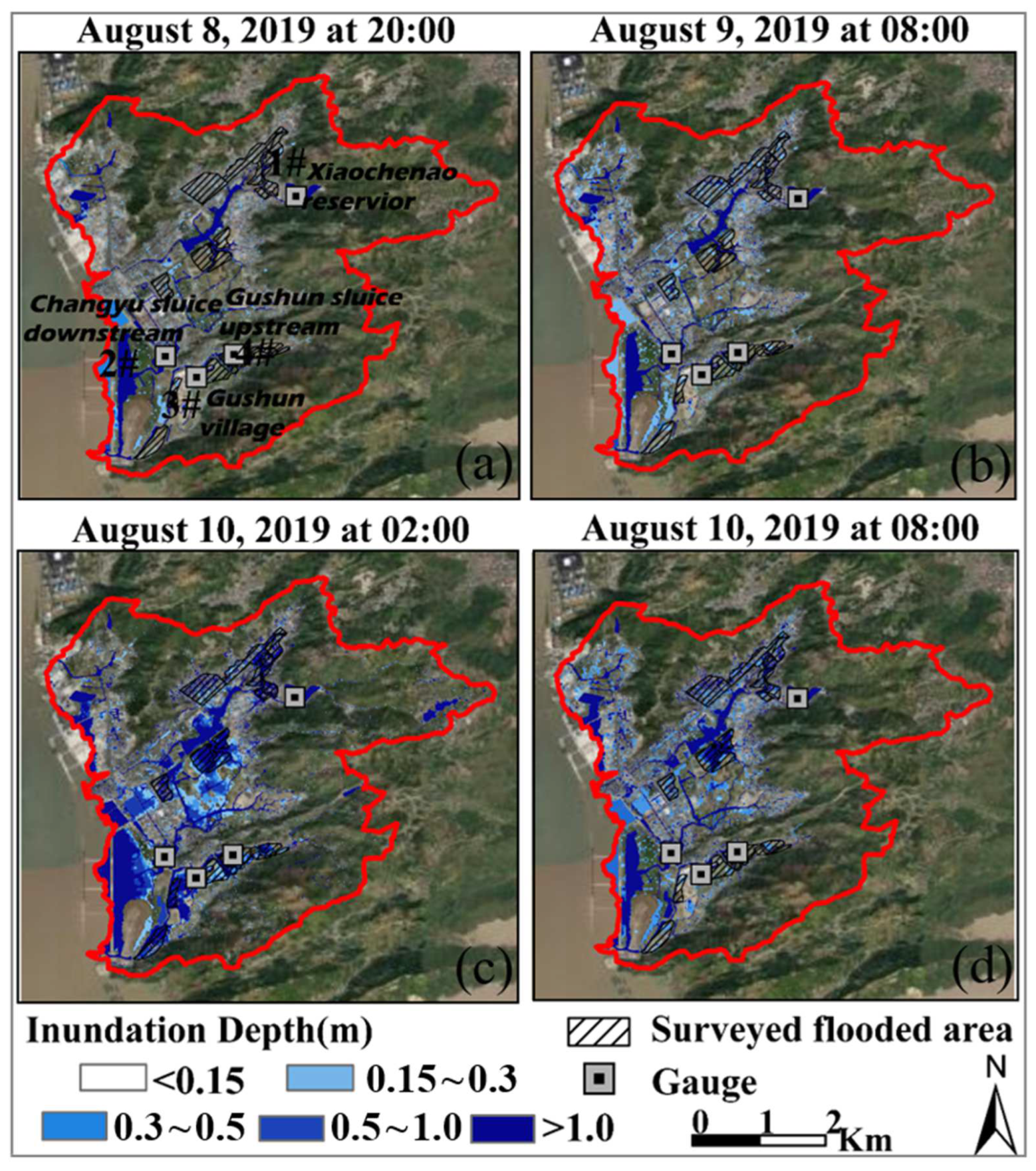
The validation is conducted by reproducing the flood event induced by Typhoon Lekima in Damaiyu Subdistrict, Yuhuan. The simulation was undertaken on the 3 m DEM for the entire 25.8 km² domain. Driven by the rainfall measured at the Gauge stations (Figure 8a) and tidal boundary conditions (Figure 8b), the simulation was run for 48 h between 08:00 a.m. on 8 and 08:00 a.m. on 10 of August. Figure 9 shows the predicted inundation extent and depth maps for the Damaiyu Subdistrict at different output times, compared with the surveyed flood extent as outlined by the thin black lines. At t = 12 h, as shown in Figure 9a, some low-lying areas. such as Chenbei Village, were inundated. 12 h later (t = 24 h, Figure 9b), water depths at most of the Damaiyu Subdistrict roads exceeded 0.15 m. Figure 9c presents the maximum inundation depths until t = 42 h, at which point the maximum extent was consistent with the surveyed flood extent. The F-statistics calculated for the predicted maximum extent against the post-event survey extent is 91.56%. After the rainfall peak has passed, flooding starts to retreat gradually, as shown in Figure 9d. The simulation results confirm the model’s capability for simulating and predicting urban flooding in high-density residential areas.

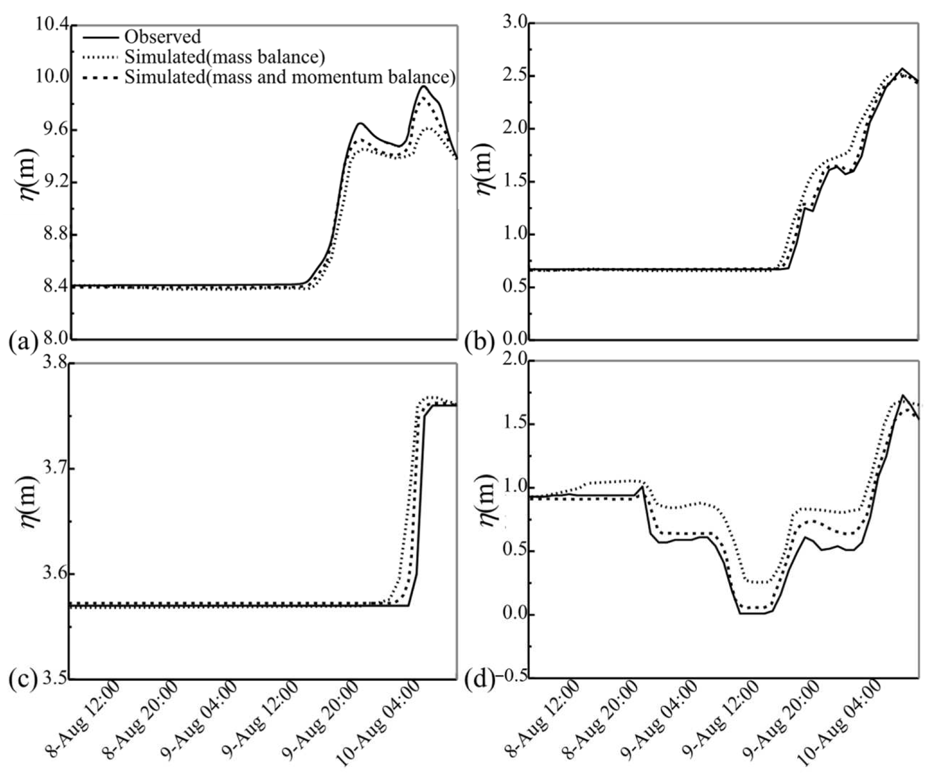
Results using both coupling approaches (i.e., source term coupling and flux term coupling) for sluicegates were further compared. Four gauge stations (named Guage 1#~4# in Figure 9) provided the time series of water levels during the flood event. As shown in Figure 10a–d, the numerical predictions from the flux term coupling approach (thin dashed line) and the source term coupling approach (thick dashed line) were compared with the observed data (solid line). It was observed that the simulation results (e.g., maximum water level and flooding arrival time) from the flux term coupling approach agreed favorably with the observed data at all of the four gauge points. The NSE and RMSE were listed in

Table 1. NSE and RMSE calculated for four gauge points.

Gauge	1#	2#	3#	4#
NSE/RMSE (source)	0.675/0.207	0.679/0.205	0.783/0.158	0.565/0.322
NSE/RMSE (flux)	0.892/0.084	0.825/0.079	0.913/0.081	0.786/0.140

. The NSE for the source term coupling approach was smaller than that for the flux term coupling approach by 14~28%. The RMSE from the flux term coupling approach was 2/5~3/5 smaller than that for the source term coupling approach. The results confirm that the flux term approach performs better than the source term coupling approach in representing hydraulic structures, such as sluicegates, as momentum exchange is effectively taken into account.

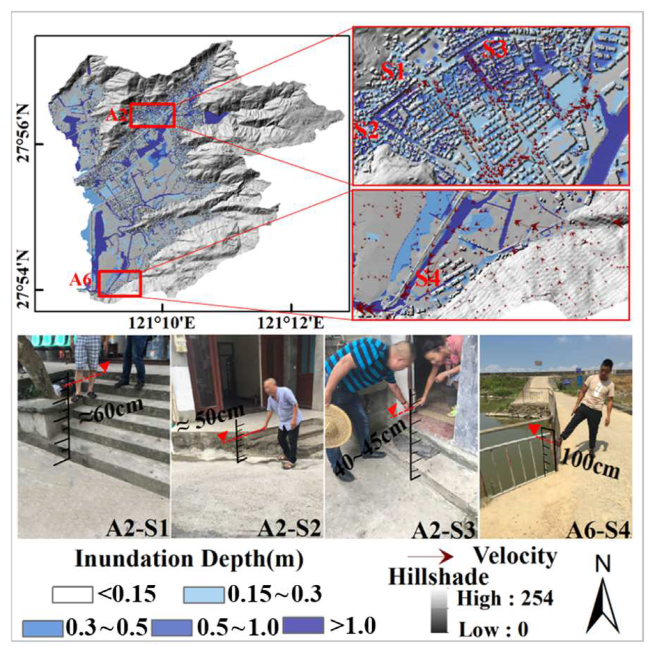
The maximum flood depths of low-lying areas surveyed by the Zhejiang Institute of Hydraulics & Estuary were used to examine the simulation. Figure 11 shows the comparison of the predicted maximum inundation depths with the surveyed depths. Both the old town and Qingfeng gate upstream in the Damaiyu Subdistrict have suffered from severe flooding, which is marked as A2 and A6 in Figure 6. The inundation depth of more than half of the road networks in the A2 area exceeded 0.3 m. Road networks would be disrupted, since the height of a car’s air inlet is 0.25~0.35 m. The maximum inundation depths at the surveyed flooding sites (S1~S4) were extracted from the maximum inundation map and listed in

Table 2. Comparison of the observed data with simulation results.

Location	Surveyed (m)	Simulated (m)
A2-S1	≈0.60	0.68
A2-S2	≈0.50	0.59
A2-S3	0.40~0.45	0.48
A2-S4	>1.00	1.39

. It was observed that the simulation results compared well with the surveyed data.

4.2. Scenario Simulations

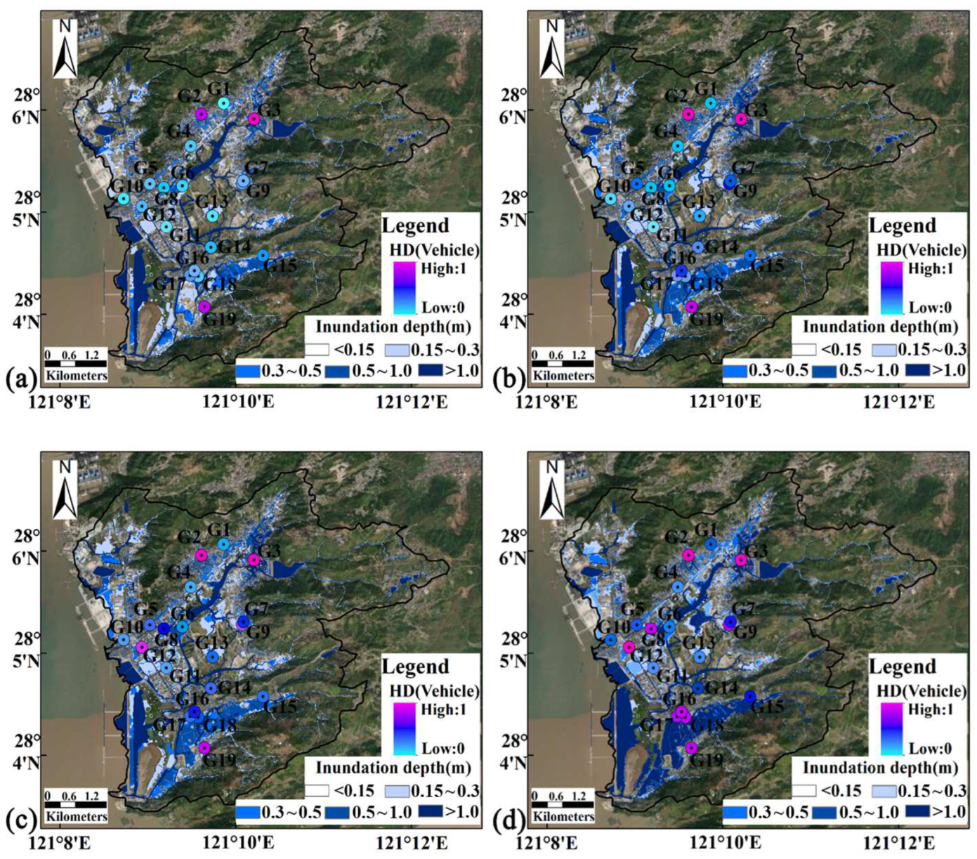
To assess the flood impact on individual objects, we constructed hydrological scenarios based on the Chicago rainfall processes, as shown in Figure 8a (i.e., 20-year, 50-year, 100-year and 200-year) combined with the “9711” tide level process (Figure 8b). The gauge points for monitoring the flood hazard risk to vehicles at certain locations (e.g., schools, bus stops, clinics and refuges) are shown in Figure 12, and their coordinates are listed in

Table 3. Information on Gauge points.

Gauge Point	Location	Lon(°)	Lat(°)
G1	Xinmin School	121.167	28.102
G2	Damaiyu Health Center	121.162	28.100
G3	Chenbei Village Bridge	121.173	28.099
G4	Damaiyu Police Station	121.160	28.095
G5	Chenyu Post Office	121.152	28.088
G6	Taizhou Customs Office (Yuhuan)	121.158	28.088
G7	Xinmin Community	121.171	28.089
G8	Damaiyu Tax Office	121.155	28.088
G9	Qinglan Community Center	121.171	28.088
G10	Damaiyu Port	121.147	28.086
G11	Yutai Disaster Relief Center	121.155	28.081
G12	Damaiyu Community	121.150	28.084
G13	Wuyi Village Economic Cooperative	121.165	28.083
G14	Wuyi Village Home Elderly Care Center	121.164	28.077
G15	Aoli Village Committee	121.175	28.076
G16	Gushun Health Service Center	121.161	28.073
G17	Gushun Bus Station	121.160	28.072
G18	Gushun Middle School	121.162	28.072
G19	Shiwumu Village Committee	121.163	28.067

. The exposure of individual objects (e.g., roads, buildings) can be spatially identified by overlaying the predicted flood inundation (extent and depth).

The flood hazard risk to vehicles at the above gauge points was assessed using Equations (16) and (17). Figure 12 presents the maximum inundation depths over the whole domain and the hazard degree of vehicles at the gauge points under the above extreme scenarios. Among all of the scenarios under consideration, the least and worst serious scenario is clearly given by the 20-year Chicago rainfall processes and 100-year Chicago rainfall processes, respectively. In general, the maximum inundations are gradually increased with rainfall intensify. As shown in Figure 12a, severe flooding would potentially hit most of the whole study domain under the scenario with a 20-year return period. The hazard degree of Gauge G2, G3 and G19 (i.e., Damaiyu Health Center, Chenbei Village Bridge and Shiwumu Village Committee) in Figure 12a is approaching 1.0. At the same time, half of the gauge points are at risk of vehicle instability under the scenario with a 200-year return period. It is worth mentioning that vehicles at gauge point G11 (i.e., Yutai Disaster Relief Center) could escape from severe flooding under each scenario. Table 3 lists the predicted statistical results for impacted road length under different return period floods. A critical threshold (i.e., 30 cm) is used to describe the relationship between inundation depth and road disruptions [56]. When the inundation depth exceeds the critical threshold, road flooding would occur and then cause transportation to be affected. As expected, flooding’s impact on transportation is directly related to the magnitude of precipitation. With the increase in return periods, the impacted road length gradually increased.

According to the field survey, the category of affected buildings in the study area is residential houses, industrial plants, and shops on the first floor. The average height of the buildings on the first floor is about 15 cm above the ground, according to Code for Design of Residential Buildings (GB 50096-2011). The new coupled model treats internally submerged houses as exposed, using the submerged water level minus the house’s height above ground (sill and step heights). The number of residential houses exposed to different inundation depths is shown in

Table 4. Statistics on length (m) (percentage %) of roads for different inundation depth under normal case.

	P (year)	20	50	100	200
h (m)
<0.15		246.4 (77.9)	229.6 (72.6)	218.3 (69.0)	210.7 (66.6)
0.15–0.3		23.4 (7.4)	25.0 (7.9)	26.6 (8.4)	29.7 (9.4)
0.3–0.5		18.3 (5.8)	23.7 (7.5)	25.9 (8.2)	26.6 (8.4)
0.5–1.0		16.5 (5.2)	19.6 (6.2)	23.7 (7.5)	25.9 (8.2)
>1.0		11.7 (3.7)	18.4 (5.8)	21.8 (6.9)	23.4 (7.4)

. The maximum number of impacted buildings from the scenario with a 200-year return period is estimated to be approximately 35% more than in the scenario with a 20-year return period. Results show that the number of affected buildings obviously increased with the increase in the rainfall return period.

Simulation result comparison from various flood scenarios brings three main findings. Firstly, the inundation depth may exceed traffic critical threshold while the hazard degree is low at most of the gauge points. Flooding may affect transportation but not pose a direct threat to vehicles themselves. Secondly, the interrupted length of road networks under the worst scenario is approximately two times more than that due to the least serious scenario. This indicates that the transportation system and associated moving vehicles on affected roads may be easily subject to the direct inundation impact of low-frequency floods. Lastly,

Table 5. Statistics on the number (percentage %) of buildings for different inundation depth under normal case.

	P (year)	20	50	100	200
h (m)
<0.15		5678 (81.6)	5601 (80.5)	5490 (78.9)	5232 (75.2)
0.15–0.3		362 (5.2)	383 (5.5)	424 (6.1)	494 (7.1)
0.3–0.5		348 (5.0)	362 (5.2)	390 (5.6)	473 (6.8)
0.5–1.0		299 (4.3)	313 (4.5)	334 (4.8)	404 (5.8)
>1.0		271 (3.9)	299 (4.3)	320 (4.6)	355 (5.1)

indicates that the number of affected buildings under the least serious scenario is 1/3 less than the impacted building number under the worst scenario, demonstrating a nonlinear relationship between inundation extents and the number of affected buildings.

4.3. Pre-Discharge Analysis

Pre-discharge of sluicegates should be basedon the premise of avoiding waterlogging, lift the gates to release flooding into the downstream of channel in advance according to scheduling operation [57]. To investigate the effects of pre-discharge on flood mitigation, simulations are conducted on different sluice schedule schemes The sluice gates in the study area often pre-discharge 1 h after receiving flood warning messages. Therefore, 1-h pre-discharge of sluice gates could be considered as a normal/reference case for baseline simulation. Besides, two more cases (i.e., in-advance 0.5 h pre-discharge and delayed 0.5 h pre-discharge) are considered. The new flood model is applied to predict the flood impact on certain objects under three sluicegate pre-discharge scenarios.

4.3.1. Pre-Discharge Results

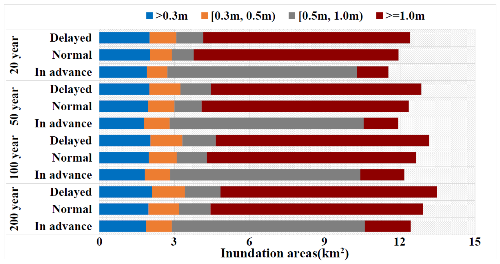
The inundation areas of three pre-discharge cases under different scenarios were shown in Figure 13. The maximum inundation extent resulting from in-advance 0.5 h pre-discharge under the least serious flood scenario is estimated to be 1.25 km², with the corresponding averaged of maximum inundation depth being 1.42 m. Twelve percent areas would be inundated with a maximum depth greater than 1 m. Furthermore, delayed 0.5 h pre-discharge of sluicegates under the worst flood scenario would lead to a much larger inundation area of 8.64 km², with an average maximum depth of 2.56 m. The whole domain inundated, exceeding 5 m, would increase fivefold to 65%.

RMSE and F-statistics of the maximum inundation extents under advance and delayed cases in each designed scenario are listed in

Table 6. RMSE and F-statistics calculated for the predictions under different pre-discharge cases in the each designed scenarios.

Pre-Discharge Case	In Advance/Delayed
Return Period (Year)	20	50	100	200
RMSE (m)	0.419/0.495	0.372/0.407	0.294/0.365	0.199/0.312
F-statistic (%)	51.75/36.89	58.63/43.92	67.19/45.37	71.36/48.69

. Under each scenario, the RMSEs increase and F-statistics decrease when the pre-discharge case transforms from advance to delayed. Under the worst scenario, the F-statistics calculated for the advanced and delayed case is about 71% and 49%, respectively. This may directly demonstrate that the flood impact due to postponing the implementation of the scheduling scheme would be greater than the preventable impact of pre-discharge in advance. However, the F-statistics obtained for the advanced case under the least serious and worst scenario is about 52% and 71%, indicating that the effectiveness of pre-discharge becomes smaller as the return period increases. Meanwhile, the RMSEs obtained from the advanced and delayed case under the worst scenario are 0.199 and 0.312. The inundation depth would be aggravating under the delayed case. The pre-discharge of sluicegates before the arrival of urban flooding plays significant role in mitigating flood risk.

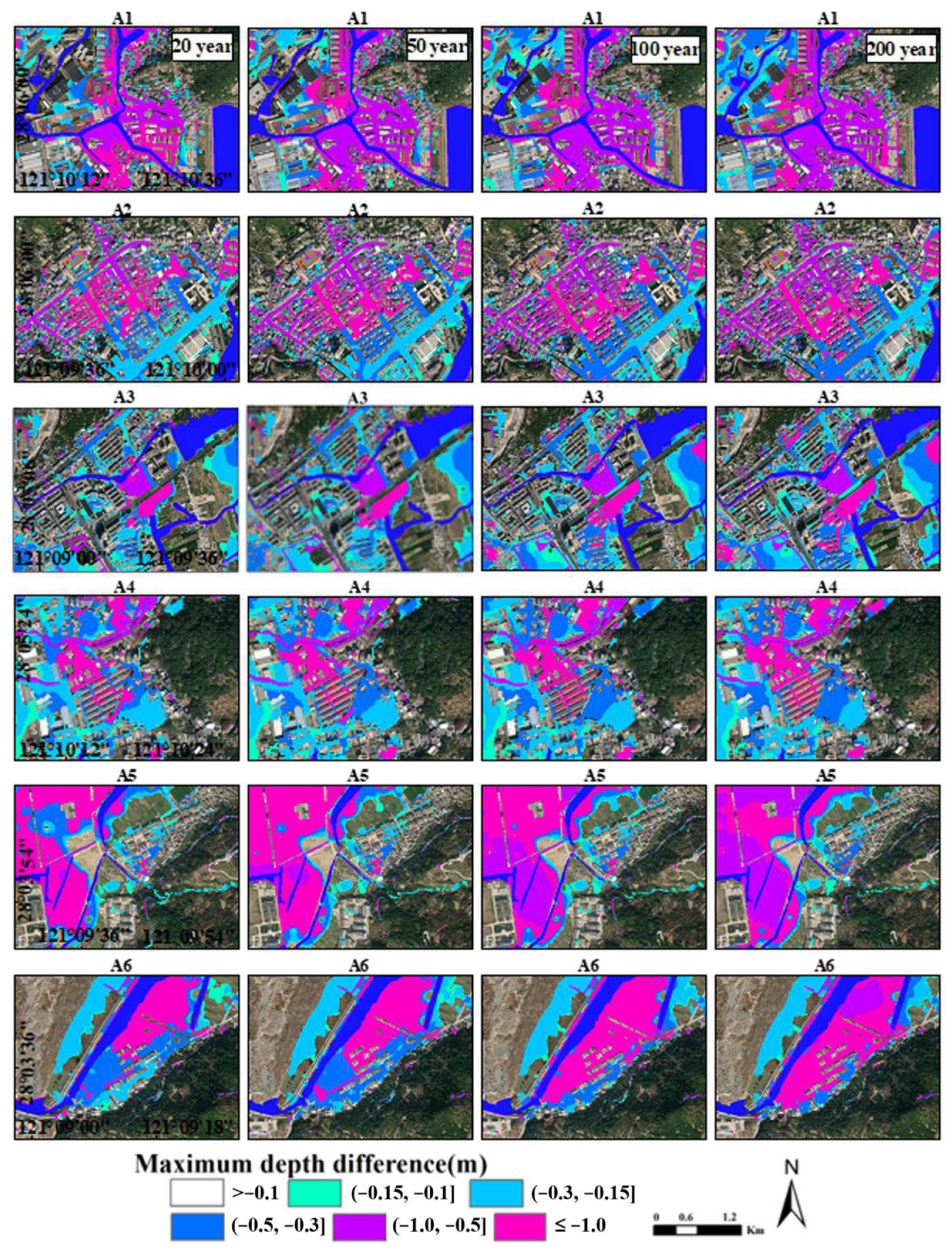
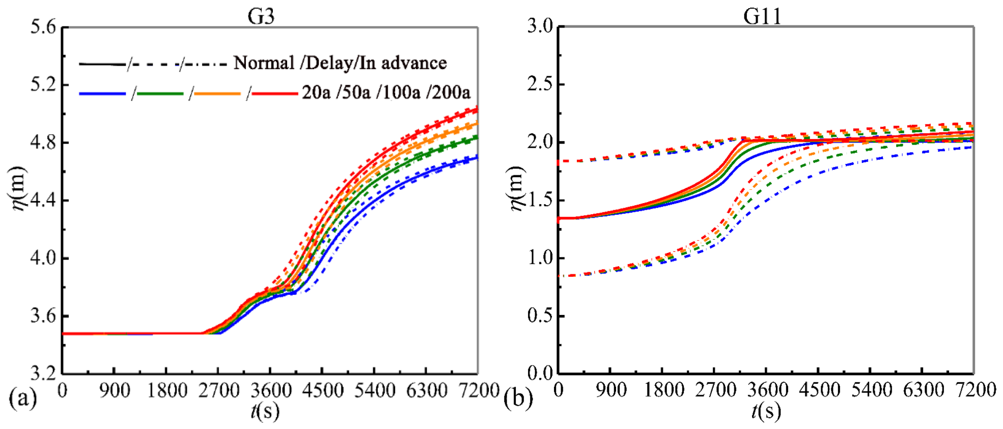
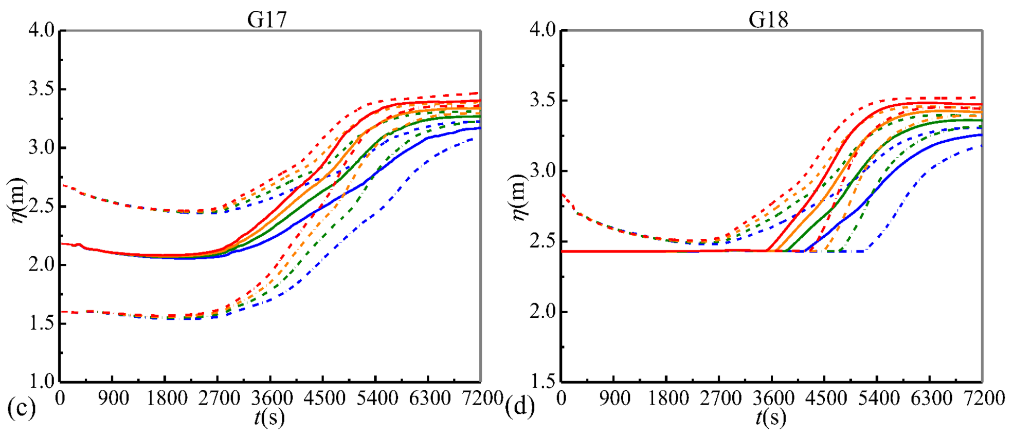
Figure 14 presents the spatial distribution of maximum depth difference on pre-discharge of sluicegates for the zoom-in surveyed flooding areas (i.e., labeled as A1~A6 in Figure 6a) throughout the simulations for each scenario. In general, the derived depth difference patterns are characterized by a high degree of consistency among the six surveyed flooding areas, albeit with various magnitudes corresponding to different rainfall return periods. By contrast, the maximum inundation (extent and depth) differences in those two more cases against the reference case are not obviously sensitive to the low-frequency flood scenarios. The results indicate that the drainage capacity of sluicegates may be subject to high rainfall-runoff in the surveyed flooding areas. Figure 15 shows the time series of water levels for certain objects at G3, G11, G17 and G18 (i.e., Chenbei Village Bridge, Yutai Disaster Relief Center, Gushun Bus Station, Gushun Middle School) under different pre-discharge cases for each designed rainfall return period. Rainfall return periods with varying pre-discharge cases may produce significantly different hydrographs for each gauge point. The maximum water level and arrival time-varying with the pre-discharge cases for each return period at those four gauge points. However, the effect of pre-discharge of sluicegates is gradually weakened as the arrival time of the maximum inundation extent. Thus, high rainfall-runoff with poor drainage systems would induce concern for urban flooding in residential areas.

4.3.2. Exposure Assessment

The predicted flood characteristics under the three pre-discharge cases mentioned above are integrated with the road, building, and facility datasets to evaluate the potential exposures, respectively. The exposure of individual objects can be spatially identified using the approaches introduced in Section 2.4. The objects exposed to different pre-discharge cases are summarized in

Table 7. Exposure estimations under two more cases against the reference case.

Case		Pre-Discharge 1 h				Pe-Discharge 0.5 h in Advance				Delayed Pre-Discharge 0.5 h
		20a	50a	100a	200a	20a	50a	100a	200a	20a	50a	100a	200a
Road (km)		46.5	61.7	71.4	75.9	32.3	57.2	69.8	73.6	53.9	69.7	76.6	80.2
Building		1280	1357	1468	1726	1065	1336	1367	1671	1369	1779	1830	1905
Public facility	G1												✓
	G4			✓	✓			✓			✓	✓	✓
	G5		✓	✓	✓			✓	✓		✓	✓	✓
	G18			✓	✓			✓	✓	✓	✓	✓	✓
Health facility	G2	✓	✓	✓	✓		✓	✓	✓	✓	✓	✓	✓
	G11											✓	✓
	G14			✓	✓			✓			✓	✓	✓
	G16		✓	✓	✓		✓	✓	✓	✓	✓	✓	✓
Traffic facility	G3	✓	✓	✓	✓		✓	✓	✓	✓	✓	✓	✓
	G17	✓	✓	✓	✓			✓	✓	✓	✓	✓	✓
Commercial facility	G6												✓
	G8		✓	✓	✓		✓	✓	✓		✓	✓	✓
	G10		✓	✓	✓			✓	✓	✓	✓	✓	✓
	G13			✓	✓			✓	✓	✓	✓	✓	✓
Residential facility	G7	✓	✓	✓	✓			✓	✓	✓	✓	✓	✓
	G9	✓	✓	✓	✓			✓	✓	✓	✓	✓	✓
	G12		✓	✓	✓		✓	✓	✓		✓	✓	✓
	G15	✓	✓	✓	✓			✓	✓	✓	✓	✓	✓
	G19	✓	✓	✓	✓		✓	✓	✓	✓	✓	✓	✓

. From the estimation results in the worst scenario, the inundated roads have been decreased by 3.0% but increased by 5.7% against the reference case, under the advance case and delayed case, respectively. Similarly, the exposure buildings can also be spatially identified. Nearly 30% of buildings were affected under the delayed case in the worst scenario. The number of affected buildings was reduced by almost 1/3 under the advance case in the scenario with 20-years return period.

Exposure analysis data at sensitive areas (e.g., the certain public, health, traffic, commercial and residential facilities) are summarized in Table 7. From the results, the exposure extent of the facilities changes correspondingly with the adoption of pre-discharge cases for each return period. For example, G2 (in health facilities), G3 and G17 (in traffic facilities), G7, G9, G15 and G19 (in residential facilities) are impacted in the scenario with a 20-year return period under the normal case. However, the scenario with a 20-year return period, as considered, may avoid affecting all the gauge points under the pre-discharge 0.5 h in the advanced case. Similarly, all of the gauge points may be hit under the delayed case in the scenario with a 200-year return period. However, G1 and G4 (in public facilities), G11 and G14 (in traffic facilities) may avoid the predicted flooding resulting from the scenario under the pre-discharge 0.5 h in the advanced case.

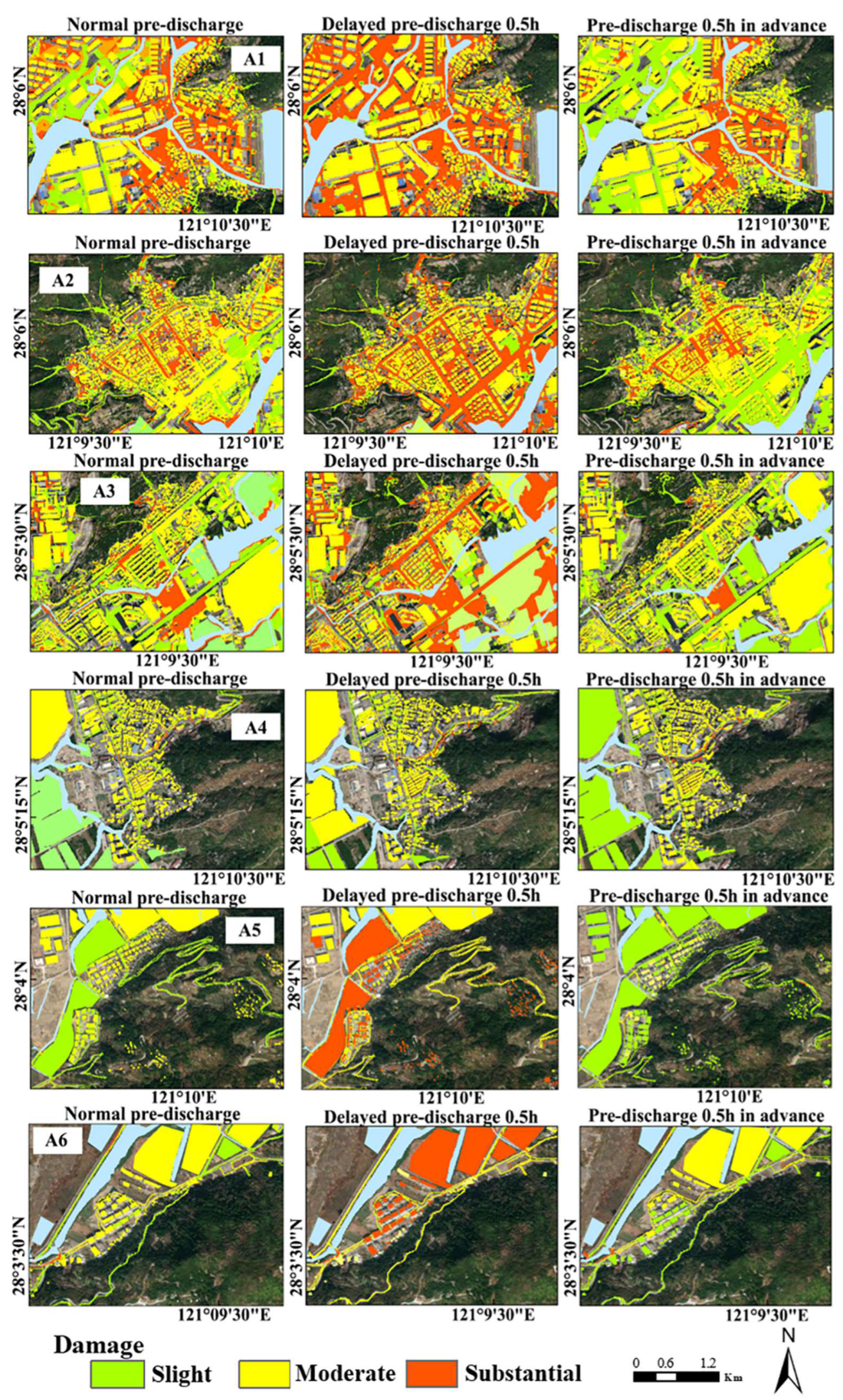
4.3.3. Damage Assessment

Based on depth-damage curves in Figure 5, the effects of hydraulic structures on individual objects are further quantified. Classification Criteria of slight, moderate and substantial damage proposed by FEMA [58] in the Hazus Flood Model are 1–10%, 11–50%, and 50–100% of damage, respectively.

The damage extents estimated for individual objects such as roads, buildings and farmland in enlarged surveyed flooding areas (i.e., labelled as A1~A6 in Figure 6a) are shown in Figure 16. In general, most of the object damage was reduced from substantial to moderate or slight damage when the case changed from the delayed case to the advanced case. The results demonstrate the indispensable effect of pre-discharge in urban flooding.

Table 8. Damage assessment under two more cases against the reference case under the worst scenario.

Case		Pre-Discharge 1 h	Pe-Discharge 0.5 h in Advance	Delayed Pre-Discharge 0.5 h
Road (km)	Slight	261.1	280.1 (+7%)	253.1 (−3%)
	Moderate	30.6	18.5 (−39%)	36.4 (+19%)
	Substantial	24.6	17.7 (−28%)	26.8 (+9%)
Building	Slight	4045	5169 (+28%)	3061 (−24%)
	Moderate	2118	1211 (−43%)	2797 (+32%)
	Substantial	793	576 (−27%)	1098 (+38%)
Farmland (km2)	Slight	1.0	1.6 (+60%)	0.5 (−50%)
	Moderate	1.2	0.7 (−42%)	1.6 (+33%)
	Substantial	0.6	0.5 (−17%)	0.7 (+17%)

presents the damage extents estimated for roads, buildings and farmlands under two more pre-discharge cases compared with the reference case. For road networks that suffered from substantial damage, against the reference case, the length of affected roads in the advance case decreased by 48% but increased by 19% under the delayed case. Regarding buildings, more than 60% of the affected buildings escaped from suffering at least moderate damage under the advanced case while adding more than 2/3 of the number of affected buildings under the delayed case. Meanwhile, for farmlands, the area of affected farmlands under the delayed case is nearly two times more than the area of affected farmlands under the advanced case. It further demonstrates the importance of the timely pre-discharge of sluicegates in urban flood risk management.

Urban flooding has become one of the most common natural hazards threatening people’s lives and assets globally due to climate change and rapid urbanization. Hydraulic structures, e.g., sluicegates and pumping stations, can directly influence flooding processes and should be represented in flood modeling and risk assessment. This study aims to present a robust numerical model incorporating a hydraulic structure simulation module to accurately predict the highly transient flood hydrodynamics interrupted by operation of hydraulic structures to support object-level risk assessment. Source-term and flux-term coupling approaches were applied and implemented to represent different types of hydraulic structures in the model. For hydraulic structures such as a sluicegate, the flux-term coupling approach may lead to more accurate results, as indicated by the calculated values of NSE and RMSE for different test cases. The model is further applied to predict different design flood scenarios with rainfall inputs created using Intensity-Duration-Frequency relationships, Chicago Design Storm, and surveyed data. The simulation results were combined with established vehicle instability formulas and depth-damage curves to assess the flood impact on individual objects in an urbanized case study area in Zhejiang Province, China.

5. Conclusions

This paper proposes a high-resolution urban flood model incorporating hydraulic structures simulation modules to accurately predict the highly transient flood hydrodynamics interrupted by operation of hydraulic structures for object-level risk assessment. An urbanized case study area in Zhejiang Province, China showed that the model can efficiently simulate multi-source flooding process induced by intense rainfall, upstream high flow and storm surge and interrupted by hydraulic structures. The key conclusions from this study are summarized as follows:

• The proposed high-resolution model successfully reproduced a flood event induced by Typhoon Lekima in Yuhuan. The flux term coupling approach for simulating the sluicegates can obtain more accurate results. The RMSE and NSE of water depths are 2/5~3/5 and 14~28% less than that from the source term coupling approach, respectively.
• The modeling framework presented here can be used to understand the effect of sluicegates on urban flood mitigation in extreme weather conditions. The simulation analysis indicates that the urban flood risks depend not only on driving force extent (e.g., rainfall intensity) but also on local drainage capacity and topographic characteristics.
• The effect of hydraulic structures on object-level hazard exposure/damage assessment using the proposed model can be estimated. The results show that a significant nonlinear relationship between inundation extents and affected build number exists and can be enhanced by the pre-discharge measures.
• Pre-discharge should be appropriately scheduled for maximizing the flood mitigation efficiency. Cases in Yuhuan show that earlier pre-discharge (e.g., 0.5 h in advance) could prevent 6.6 km of road networks, 234 buildings, 8 key facilities including schools, bus stops, clinics and refuges in a scenario with a 200-year flood return period. The substantial damage of 27% of affected buildings, 17% of inundated agricultural land and 28% of impacted road networks would be reduced.

Currently, the modeling framework proposed in this work has the potential to evaluate the impact of normal/extreme floods at the object level considering operation of hydraulic structures during floods caused by multiple sources, such as intense rainfall, high upstream flows, or storm surges. However, other relevant factors, such as drainage systems and pollutants, may influence the development process of urban flooding, which should be further considered and incorporated into the modeling framework in the future.

References

- Wang, G.; Wang, D.; Trenberth, K.E.; Erfanian, A.; Yu, M.; Bosilovich, M.G.; Parr, D.T. The peak structure and future changes of the relationships between extreme precipitation and temperature. Nat. Clim. Chang. 2017, 7, 268–274. [Google Scholar] [CrossRef]
- Fowler, H.J.; Lenderink, G.; Prein, A.F.; Westra, S.; Allan, R.P.; Ban, N.; Barbero, R.; Berg, P.; Blenkinsop, S.; Do, H.X. Anthropogenic intensification of short-duration rainfall extremes. Nat. Rev. Earth Environ. 2021, 2, 107–122. [Google Scholar] [CrossRef]
- Mal, S.; Singh, R.; Huggel, C.; Grover, A. Introducing linkages between climate change, extreme events, and disaster risk reduction. In Climate Change, Extreme Events and Disaster Risk Reduction; Springer: Berlin/Heidelberg, Germany, 2018; pp. 1–14. [Google Scholar]
- Ahmadalipour, A.; Moradkhani, H. A data-driven analysis of flash flood hazard, fatalities, and damages over the CONUS during 1996–2017. J. Hydrol. 2019, 578, 124106. [Google Scholar] [CrossRef]
- Hallegatte, S.; Green, C.; Nicholls, R.J.; Corfee-Morlot, J. Future flood losses in major coastal cities. Nat. Clim. Chang. 2013, 3, 802–806. [Google Scholar] [CrossRef]
- Yin, J.; Ye, M.; Yin, Z.; Xu, S. A review of advances in urban flood risk analysis over China. Stoch. Environ. Res. Risk Assess. 2015, 29, 1063–1070. [Google Scholar] [CrossRef]
- Headquarters, N.F.C. Heavy Rain in Zhengzhou Breaks through the Historical Extreme Value of Hourly Rainfall in Mainland My Country. Available online: https://m.gmw.cn/baijia/2021-07/28/1302438171.html (accessed on 1 December 2021).
- DW. Floods in Germany. Available online: https://www.dw.com/en/floods-in-germany/ (accessed on 4 November 2021).
- IPCC. Climate Change 2022: Impacts, Adaptation and Vulnerability; IPCC: Geneva, Switzerland, 2022. [Google Scholar]
- Ogie, R.; Holderness, T.; Dunbar, M.; Turpin, E. Spatio-topological network analysis of hydrological infrastructure as a decision support tool for flood mitigation in coastal mega-cities. Environ. Plan. B Urban Anal. City Sci. 2016, 44, 718–739. [Google Scholar] [CrossRef]
- Adnan, M.S.G.; Haque, A.; Hall, J.W. Have coastal embankments reduced flooding in Bangladesh? Sci. Total Environ. 2019, 682, 405–416. [Google Scholar] [CrossRef]
- Dazzi, S.; Vacondio, R.; Mignosa, P. Internal boundary conditions for a GPU-accelerated 2D shallow water model: Implementation and applications. Adv. Water Resour. 2020, 137, 103525. [Google Scholar] [CrossRef]
- Tingsanchali, T. Urban flood disaster management. Procedia Eng. 2012, 32, 25–37. [Google Scholar] [CrossRef] [Green Version]
- Ogie, R.I.; Holderness, T.; Dunn, S.; Turpin, E. Assessing the vulnerability of hydrological infrastructure to flood damage in coastal cities of developing nations. Comput. Environ. Urban Syst. 2018, 68, 97–109. [Google Scholar] [CrossRef] [Green Version]
- Ferrari, A.; Dazzi, S.; Vacondio, R.; Mignosa, P. Enhancing the resilience to flooding induced by levee breaches in lowland areas: A methodology based on numerical modelling. Nat. Hazards Earth Syst. Sci. 2020, 20, 59–72. [Google Scholar] [CrossRef] [Green Version]
- Echeverribar, I.; Morales-Hernández, M.; Brufau, P.; García-Navarro, P. Use of internal boundary conditions for levees representation: Application to river flood management. Environ. Fluid Mech. 2019, 19, 1253–1271. [Google Scholar] [CrossRef] [Green Version]
- Ratia, H.; Murillo, J.; García-Navarro, P. Numerical modelling of bridges in 2D shallow water flow simulations. Int. J. Numer. Methods Fluids 2014, 75, 250–272. [Google Scholar] [CrossRef]
- Maranzoni, A.; Dazzi, S.; Aureli, F.; Mignosa, P. Extension and application of the Preissmann slot model to 2D transient mixed flows. Adv. Water Resour. 2015, 82, 70–82. [Google Scholar] [CrossRef]
- Luo, P.; Mu, D.; Xue, H.; Ngo-Duc, T.; Dang-Dinh, K.; Takara, K.; Nover, D.; Schladow, G. Flood inundation assessment for the Hanoi Central Area, Vietnam under historical and extreme rainfall conditions. Sci. Rep. 2018, 8, 12623. [Google Scholar] [CrossRef]
- Angeloudis, A.; Falconer, R.A.; Bray, S.; Ahmadian, R. Representation and operation of tidal energy impoundments in a coastal hydrodynamic model. Renew. Energy 2016, 99, 1103–1115. [Google Scholar] [CrossRef] [Green Version]
- Innovyze. Integrated Catchment Modelling—InfoWorks ICM. Available online: https://www.innovyze.com/ (accessed on 24 March 2014).
- Agency, E.P. Environmental Fluid Dynamics Code (EFDC). Available online: https://www.epa.gov/ceam/environmental-fluid-dynamics-code-efdc (accessed on 10 November 2022).
- Brunner, G.W. Hec-ras (river analysis system). In North American Water and Environment Congress & Destructive Water; American Society of Civil Engineers: New York, NY, USA, 2002; pp. 3782–3787. [Google Scholar]
- Zhao, D.; Shen, H.; Tabios III, G.; Lai, J.; Tan, W. Finite-volume two-dimensional unsteady-flow model for river basins. J. Hydraul. Eng. 1994, 120, 863–883. [Google Scholar] [CrossRef]
- Riadh, A.; Cedric, G.; Jean, M. Telemac Modeling System: 2d Hydrodynamics Telemac-2d Software Release 7.0 User Manual; R&D, Electricite de France: Paris, France, 2014; Volume 134. [Google Scholar]
- DHI. MIKE 21—DHI. Available online: https://www.mikepoweredbydhi.com/ (accessed on 7 July 2016).
- Morales-Hernández, M.; Murillo, J.; García-Navarro, P. The formulation of internal boundary conditions in unsteady 2-D shallow water flows: Application to flood regulation. Water Resour. Res. 2013, 49, 471–487. [Google Scholar] [CrossRef]
- Cozzolino, L.; Cimorelli, L.; Covelli, C.; Della Morte, R.; Pianese, D. The analytic solution of the Shallow-Water Equations with partially open sluice-gates: The dam-break problem. Adv. Water Resour. 2015, 80, 90–102. [Google Scholar] [CrossRef]
- Sepúlveda, C.; Gómez, M.; Rodellar, J. Benchmark of discharge calibration methods for submerged sluice gates. J. Irrig. Drain. Eng. 2009, 135, 676–682. [Google Scholar] [CrossRef]
- Cui, Y.; Liang, Q.; Wang, G.; Zhao, J.; Hu, J.; Wang, Y.; Xia, X. Simulation of hydraulic structures in 2D high-resolution urban flood modeling. Water 2019, 11, 2139. [Google Scholar] [CrossRef] [Green Version]
- Xing, Y.; Liang, Q.; Wang, G.; Ming, X.; Xia, X. City-scale hydrodynamic modelling of urban flash floods: The issues of scale and resolution. Nat. Hazards 2018, 96, 473–496. [Google Scholar] [CrossRef] [Green Version]
- Toro, E.F. Shock-Capturing Methods for Free-Surface Shallow Flows; Wiley-Blackwell: New York, NY, USA, 2001. [Google Scholar]
- Toro, E.F.; Spruce, M.; Speares, W. Restoration of the contact surface in the HLL-Riemann solver. Shock. Waves 1994, 4, 25–34. [Google Scholar] [CrossRef]
- Liang, Q.; Smith, L.S. A High-Performance Integrated hydrodynamic Modelling System for urban flood simulations. J. Hydroinform. 2015, 17, 518. [Google Scholar] [CrossRef] [Green Version]
- Xia, X.; Liang, Q.; Ming, X. A full-scale fluvial flood modelling framework based on a high-performance integrated hydrodynamic modelling system (HiPIMS). Adv. Water Resour. 2019, 132, 103392. [Google Scholar] [CrossRef]
- Xia, X.; Liang, Q. A new efficient implicit scheme for discretising the stiff friction terms in the shallow water equations. Adv. Water Resour. 2018, 117, 87–97. [Google Scholar] [CrossRef]
- Xia, X.; Liang, Q.; Ming, X.; Hou, J. An efficient and stable hydrodynamic model with novel source term discretization schemes for overland flow and flood simulations. Water Resour. Res. 2017, 53, 3730–3759. [Google Scholar] [CrossRef]
- Henderson, F.M. Open Channel Flow; Macmillan: New York, NY, USA, 1996. [Google Scholar]
- Henry, H. Discussion of Diffusion of submerged jets. Trans. Proc. ASCE 1950, 115, 687–694. [Google Scholar]
- Shearman, J.; Kirby, W.; Schneider, V.; Flippo, H. Bridge Waterways Analysis Model; Federal Highway Administration: Washington, DC, USA, 1986.
- Xia, J.; Falconer, R.A.; Lin, B.; Tan, G. Numerical assessment of flood hazard risk to people and vehicles in flash floods. Environ. Model. Softw. 2011, 26, 987–998. [Google Scholar] [CrossRef]
- Chen, H.; Zhao, J.; Liang, Q.; Maharjan, S.B.; Joshi, S.P. Assessing the potential impact of glacial lake outburst floods on individual objects using a high-performance hydrodynamic model and open-source data. Sci. Total Environ. 2021, 806, 151289. [Google Scholar] [CrossRef]
- Cao, R.; Zhu, J.; Tu, W.; Li, Q.; Cao, J.; Liu, B.; Zhang, Q.; Qiu, G. Integrating aerial and street view images for urban land use classification. Remote Sens. 2018, 10, 1553. [Google Scholar] [CrossRef] [Green Version]
- Xiong, Y.; Liang, Q.; Park, H.; Cox, D.; Wang, G. A deterministic approach for assessing tsunami-induced building damage through quantification of hydrodynamic forces. Coast. Eng. 2019, 144, 1–14. [Google Scholar] [CrossRef] [Green Version]
- Chen, H.; Liang, Q.; Liang, Z.; Liu, Y.; Xie, S. Remote-sensing disturbance detection index to identify spatio-temporal varying flood impact on crop production. Agric. For. Meteorol. 2019, 269–270, 180–191. [Google Scholar] [CrossRef]
- Yin, J.; Yu, D.; Yin, Z.; Liu, M.; He, Q. Evaluating the impact and risk of pluvial flash flood on intra-urban road network: A case study in the city center of Shanghai, China. J. Hydrol. 2016, 537, 138–145. [Google Scholar] [CrossRef] [Green Version]
- Huizinga, J.; de Moel, H.; Szewczyk, W. Global Flood Depth-Damage Functions: Methodology and the Database with Guidelines; EUR 28552 EN; Publications Office of the European Union: Luxembourg, 2017. [Google Scholar]
- Yang, Y.; Ng, S.T.; Zhou, S.; Xu, F.J.; Li, H. A physics-based framework for analyzing the resilience of interdependent civil infrastructure systems: A climatic extreme event case in Hong Kong. Sustain. Cities Soc. 2019, 47, 101485. [Google Scholar] [CrossRef]
- Ahmad, S.S.; Simonovic, S.P. Spatial and temporal analysis of urban flood risk assessment. Urban Water J. 2013, 10, 26–49. [Google Scholar] [CrossRef]
- McCuen, R.H.; Johnson, P.A.; Ragan, R.M. Highway Hydrology: Hydraulic Design Series No. 2; National Highway Institute: Washington, DC, USA, 1996.
- Brakensiek, D.; Onstad, C. Parameter estimation of the Green and Ampt infiltration equation. Water Resour. Res. 1977, 13, 1009–1012. [Google Scholar] [CrossRef]
- Rawls, W.J.; Brakensiek, D.L.; Miller, N. Green-Ampt infiltration parameters from soils data. J. Hydraul. Eng. 1983, 109, 62–70. [Google Scholar] [CrossRef] [Green Version]
- Keifer, C.J.; Chu, H.H. Synthetic storm pattern for drainage design. J. Hydraul. Div. 1957, 83, 1332-1–1332-1325. [Google Scholar] [CrossRef]
- Pan, Z.-h.; Liu, H. Extreme storm surge induced coastal inundation in Yangtze Estuary regions. J. Hydrodyn. 2019, 31, 1127–1138. [Google Scholar] [CrossRef]
- Nash, J. River flow forecasting through conceptual models, I: A discussion of principles. J. Hydrol. 1970, 10, 398–409. [Google Scholar] [CrossRef]
- Pregnolato, M.; Ford, A.; Wilkinson, S.M.; Dawson, R.J. The impact of flooding on road transport: A depth-disruption function. Transp. Res. Part D Transp. Environ. 2017, 55, 67–81. [Google Scholar] [CrossRef]
- Zheng, S.; Zhong, Z.; Zou, Q.; Ding, Y.; Yang, L.; Luo, X. Study on Countermeasures for Risks of Flood Resources Utilization in the Three Gorges Project. In Flood Resources Utilization in the Yangtze River Basin; Springer: Singapore, 2021; pp. 325–345. [Google Scholar]
- FEMA. Multi-Hazard Loss Estimation Methodology, Flood Model, HAZUS, Technical Manual; FEMA, Mitig Div: Washington, DC, USA, 2013; Volume 569.
Figure 1.
Framework for object-level assessment of flood impact, considering the operation of hydraulic structures.
Figure 2.
Flow through a sluicegate: (a) free flow; (b) submerged flow.
Figure 3.
Calculating fluxes through a line/polyline hydraulic structure using a flux-term coupling approach on a 2D computational grid.
Figure 4.
Diagram of the source coupling approach for point/polygon hydraulic structures.
Figure 5.
Adopted water depth-damage curves for different objectives considered in this work: (a) Building; (b) Farmland; (c) Road.
Figure 6.
Detailed map of the study area illustrating (a) location of the domain, DEM and surveyed flooding area, (b) land use and location of sluice gates.
Figure 7.
Time series of driving forces during Typhoon Lekima (2019): (a) hourly and accumulated rainfall; (b) tidal level at the Qinglan Estuary.
Figure 8.
The driving forces of the model under extreme scenarios: (a) rainfall; (b) tidal level.
Figure 9.
Predicted inundation extent and depth maps in the study area: (a) t = 12 h; (b) t = 24 h; (c) the maximum inundation map; (d) t = 48 h.
Figure 10.
Comparison of the simulation results from the source coupling approach and flux coupling approach with observed data at gauge stations: (a) 1#; (b) 2#; (c) 3#; (d) 4#.
Figure 11.
Comparison of simulated results and survey data of maximum inundation depth in the study area.
Figure 12.
HD at each gauge point and inundation maps for different rainfall periods: (a) 20 year; (b) 50 year; (c) 100 year; (d) 200 year.
Figure 13.
Inundation extents of three pre-discharge cases under different scenarios.
Figure 14.
Difference between the maximum inundation depth difference on pre-discharge 0.5 h in advance and delayed pre-discharge 0.5 h case calculated against the prediction under the normal case in the zoom-in surveyed flooding areas: A1 (Chenbei village), A2 (Old town), A3 (Intersec-tion of Xingzhong Road and Longshan Road), A4 (Xinmin community), A5 (Shiwumu village) and A6 (Huanhai village).
Figure 15.
Time series of water levels of the different pre-discharge cases under different designed scenarios at (a) G3; (b) G11; (c) G17; (d) G18.
Figure 16.
Object-based damage assessment for different pre-discharge cases under the worst scenario in the zoom-in surveyed flooding areas: A1 (Chenbei village), A2 (Old town), A3 (Intersec-tion of Xingzhong Road and Longshan Road), A4 (Xinmin community), A5 (Shiwumu village) and A6 (Huanhai village).