1. Introduction
The OPF is still a significant subject in the community of power-system researchers since it began almost half a century ago. The OPF is considered a nonlinear, multi-dimensional, and large-scale problem in the operation of power systems. The primary purpose of the OPF is to optimize a particular objective function by meeting a group of operational and physical restrictions mandated by equipment and power system restrictions. The objective function can be divided into single- and multi-objective functions. Examples of objective functions include the fuel costs for generators, their emission rates, the electricity grid’s losses, and the security index of the voltage. Equality and inequality constraints involve power-balance equations and limitations on all state and control variables. The control variables involve the active power of the generator, the bus voltage of the generator, the transformer tap ratios, and the VAR (volt–ampere reactive) compensators, whereas the state variables include the reactive power outputs from the generators, the bus load voltages, and the network line flow. Consequently, the electric utilities use the OPF issue as an essential tool to describe secure and economically advantageous operational conditions for power systems.
The earliest OPF problem was solved using traditional mathematical programming techniques, successfully proving their viability [
1]. Conventional methods of optimization are used for solving the OPF problem, such as the method of Newton [
1], the method of gradient projection [
2], the method of linear programming [
3], and the method of interior point [
4]. The conventional optimization methods are accompanied by many difficulties reported in [
5]. Due to the continuously developing optimization issues, several techniques have been established to solve the OPF; artificial intelligence techniques and meta-heuristic, search-based optimization methods have been developed for solving the OPF issue. Search-based optimization methods have been recently used for solving the OPF problem, such as the particle swarm optimizing algorithm (PSO) [
6,
7], genetic algorithms method (GA) [
8], enhanced genetic algorithms method [
9], differential evolution algorithm method [
10,
11], gravitational searching algorithm method (GSA) [
12,
13], improving colliding bodies algorithm [
14], multi-phase searching optimization algorithm [
15,
16], improved PSO [
17], fuzzy-based hybrid PSO approach [
18], biogeography-based optimizing algorithm [
19], black-hole optimization algorithm [
20], harmony search optimization algorithm [
21], imperialist competitive optimization algorithm [
22], grey wolf optimization [
23], PSO hybrid with GSA algorithm [
24], and the bee colony optimization algorithm [
25]. Several multi-objective functions for the OPF problem were introduced in [
11,
17,
18,
23].
Currently, there is an increase on the grid in the use of RESs such as solar and wind energy [
26,
27]. Although RESs have benefits such as lowering pollution and saving resources, the consequent rise in load uncertainty and associated uncertainty in power production have created new difficulties in the operation and distribution of power networks. To successfully integrate those sources into the grid and provide a secure and lucrative power market, it is critical to manage them properly [
26,
28]. Therefore, their stochastic nature must be considered while integrating these sporadic RESs into the grid. Solving the OPF problem has been significantly difficult because of the uncertainties of the added RESs to the system. Furthermore, solving the OPF is computationally intensive and impractical because it necessitates running numerous simulations to consider most of the possible operating conditions. Both traditional and intelligence-based techniques (deterministic techniques) for solving the OPF issue have been mentioned in the previous paragraph. Still, the probabilistic techniques must be considered to address the uncertainty of the RESs.
Probabilistic techniques can offer improved solutions and appropriate accuracy when considering uncertainties [
29,
30]. Therefore, it is preferred that the POPF problem is solved using a probabilistic approach rather than the deterministic point of view, as thoroughly reviewed by Ramadhani et al. in [
31] and Prusty and Jena in [
32,
33]. In power systems with numerous PV and wind units, many probabilistic techniques are used in solving the OPF issue. To obtain the PDF of the PV system’s output power, the two-point estimate method (2PEM), dependent on the moments’ technique, was introduced in [
34]. However, the moments’ method sometimes produces estimates which do not fall within the parameter space, resulting in the solution becoming unreliable. The Cornish–Fisher expansion was presented in [
35] to handle the uncertainties of the PV sources Still, this method does not produce accurate estimations when handling problems that contain non-continuous return functions and complex structures [
36]. A POPF problem with wind power inserted into the system was presented in [
37], and the heuristic approach was used to calculate the PDF of the wind speed. However, real data must be available to calculate the PDF accurately. The kernel-density estimation technique estimated the wind speed probability distribution [
38]. However, this approach is impractical since the density estimate depends on where the bins are when they are initially placed. The number of bins increases exponentially as the number of dimensions increases. According to the Latin hypercube random sampling technique, the mean–variance skewness methodology for stochastic and nonconvex OPF incorporating wind energy was developed in [
39]. However, this approach is hampered by the sample points’ statistical dependencies, and it does not appear to be noticeably better than other random sample methods for sensitive analysis. To obtain the PDF of the power produced from a wind energy system, the Monte Carlo Simulation (MCS) and its variations were taken into consideration in [
40,
41]. The MCS technique was used to develop an OPF issue for a power system with PV and WE units [
42].
This study formulates and solves the POPF issue with a hybrid power system that contains wind and solar energy sources. These are the primary contributions made in this paper:
Implement and solve the POPF approach while allowing RESs to become more integrated into the electricity grid using Artificial Gorilla Troops Optimization (GTO).
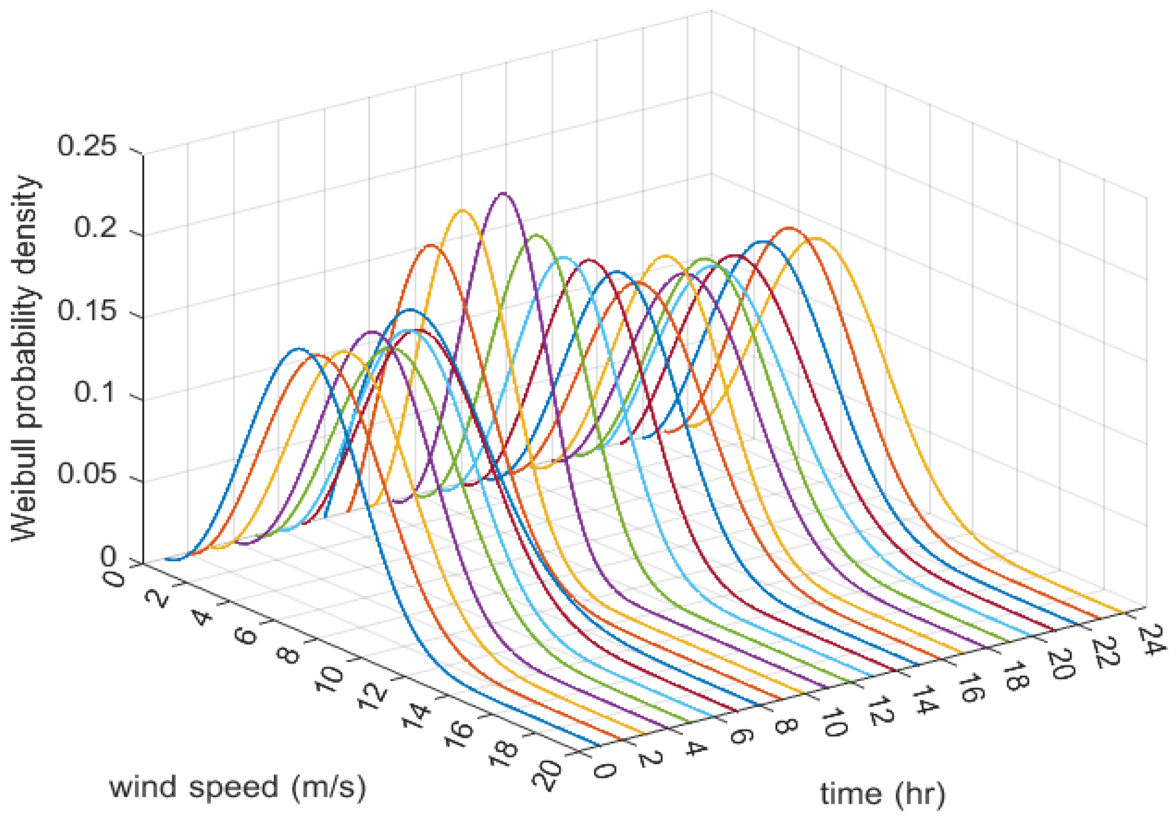
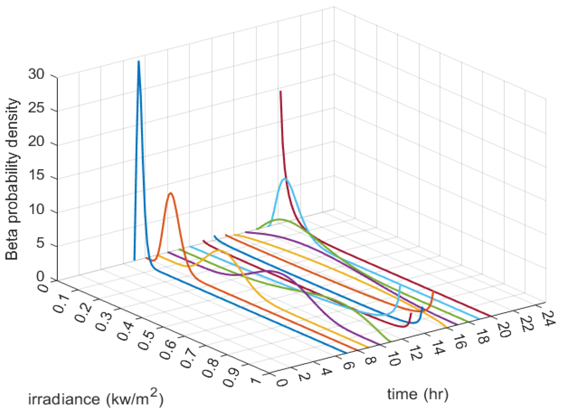
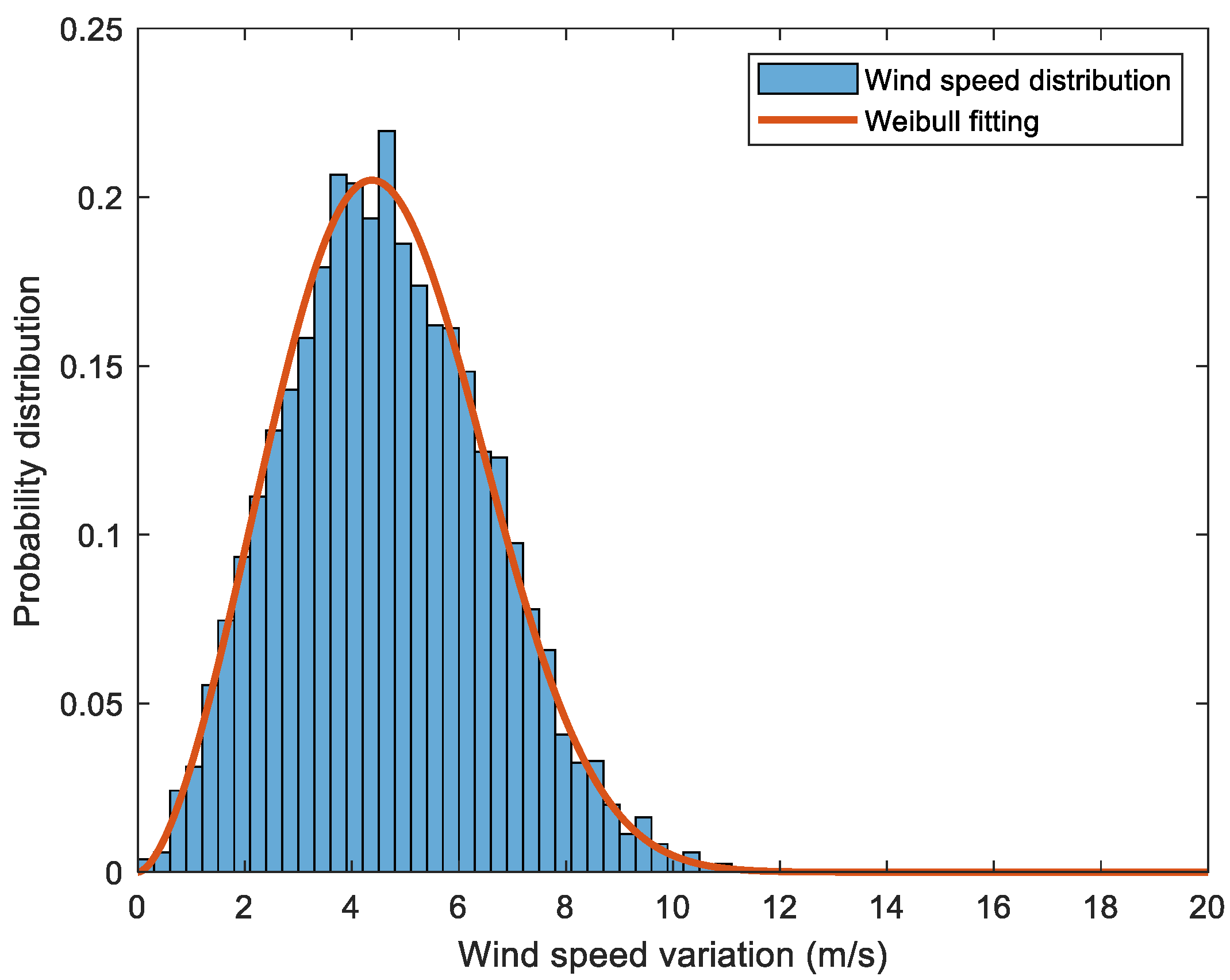
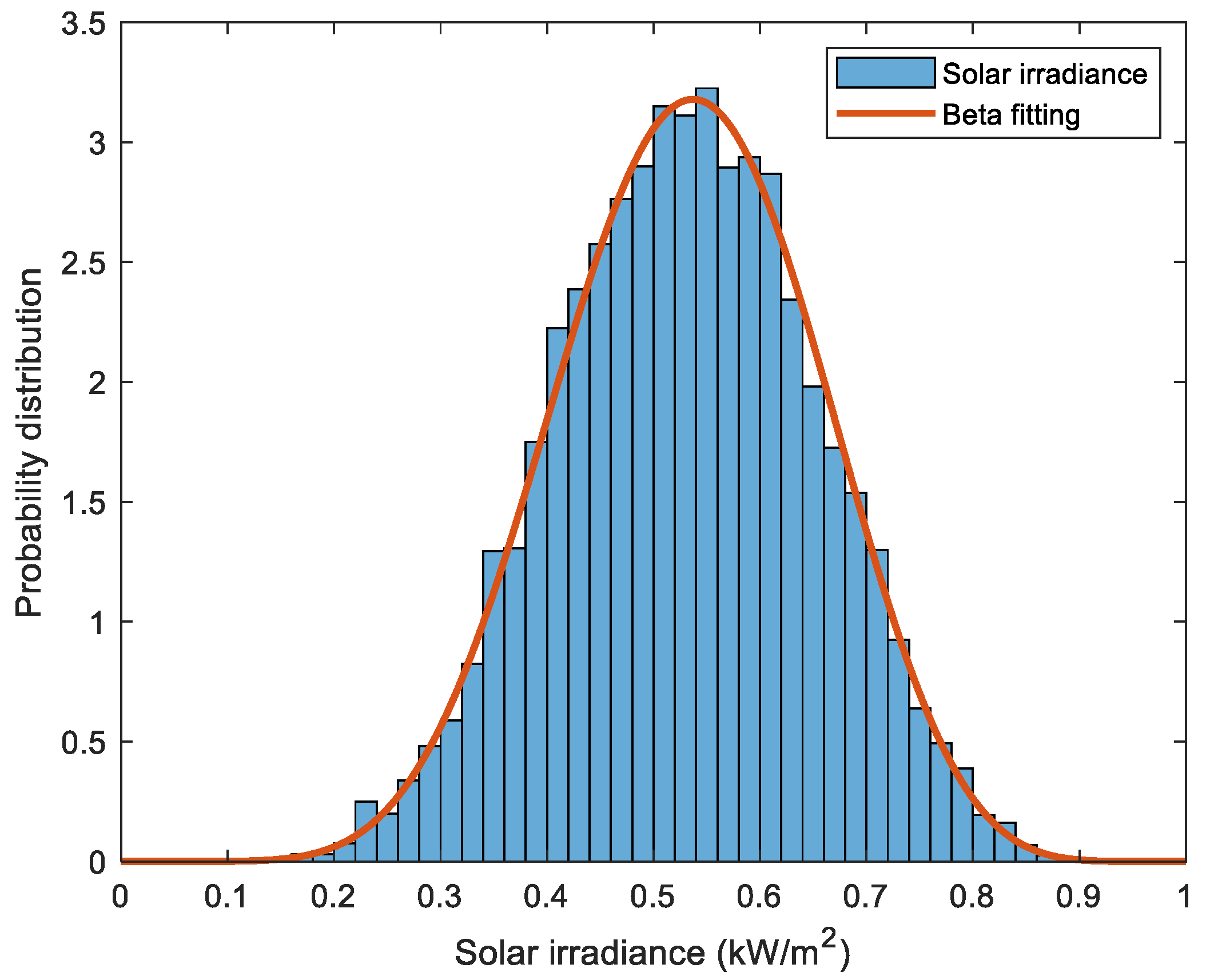
Obtain actual historical data for the summers of four years (2018, 2019, 2020, and 2021). The whole data are used to mimic a more accurate 24-h summer day and provide curve-fitting for each hour of data for PV and wind using the Beta and Weibull PDFs, respectively.
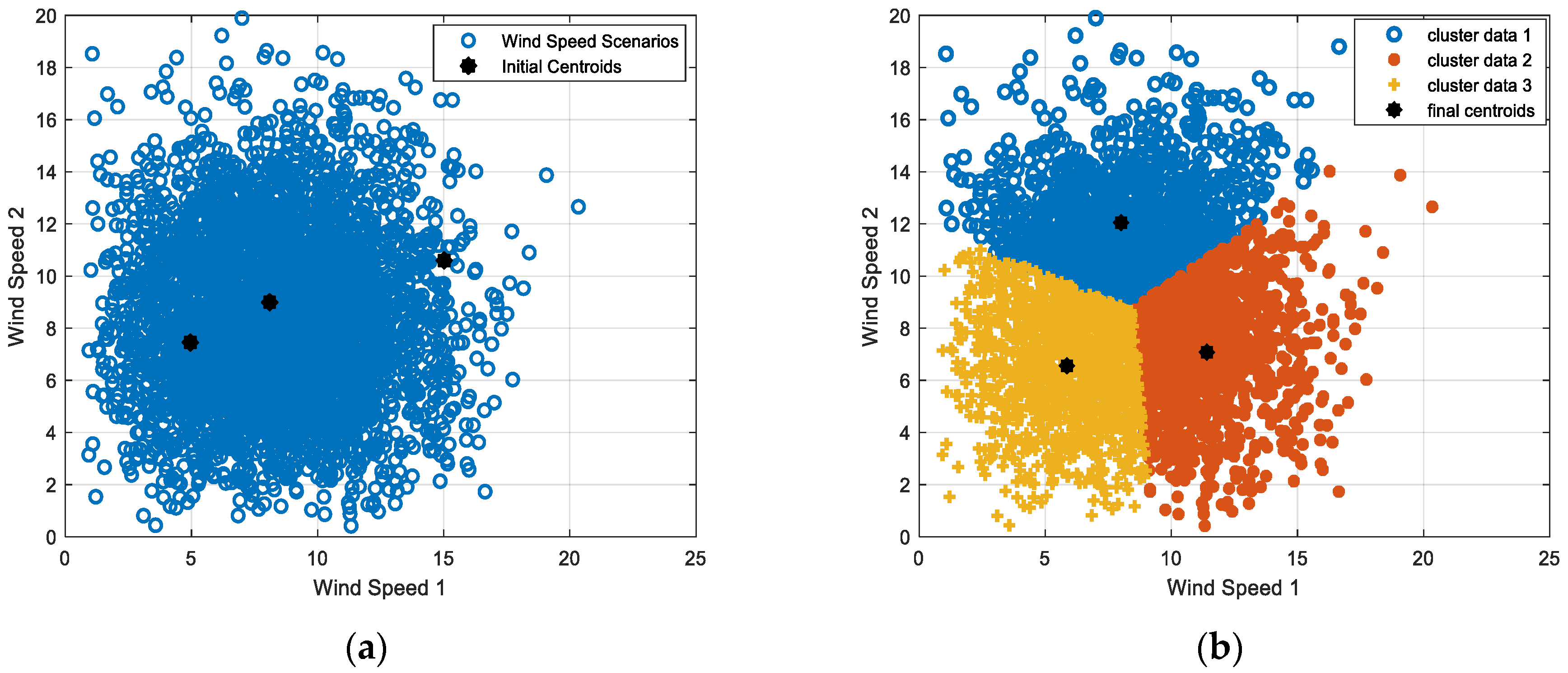
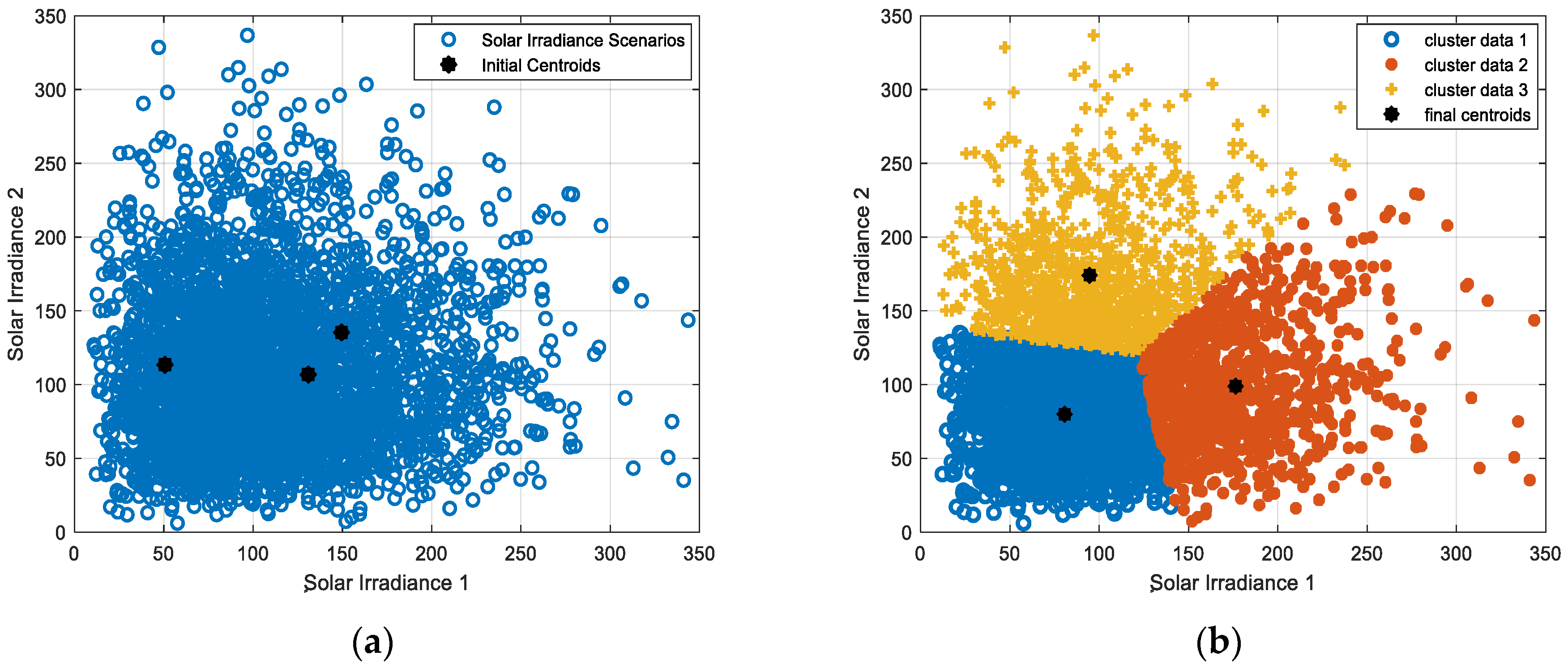
Combine the MCS with the K-means clustering method to reduce the significant computational time.
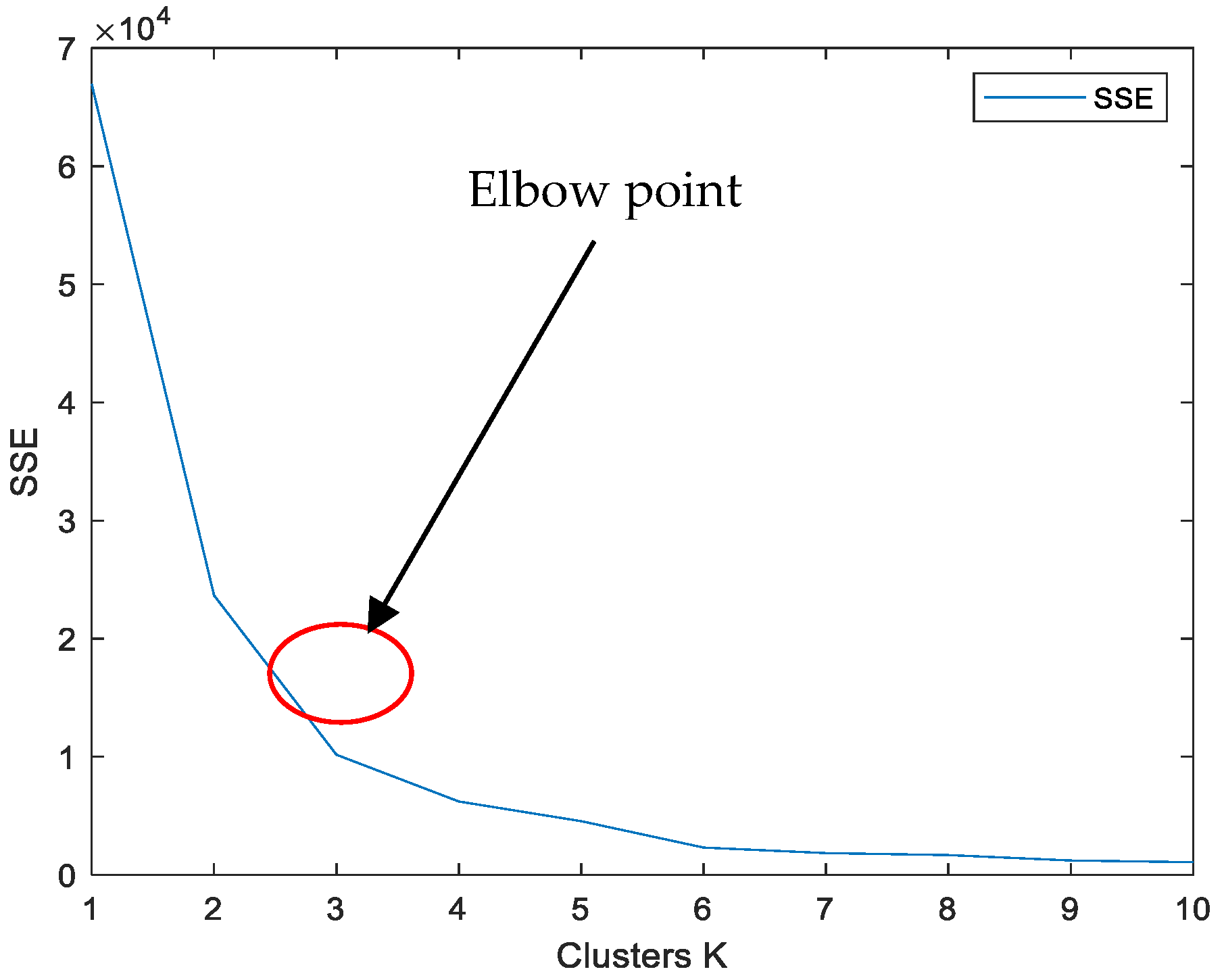
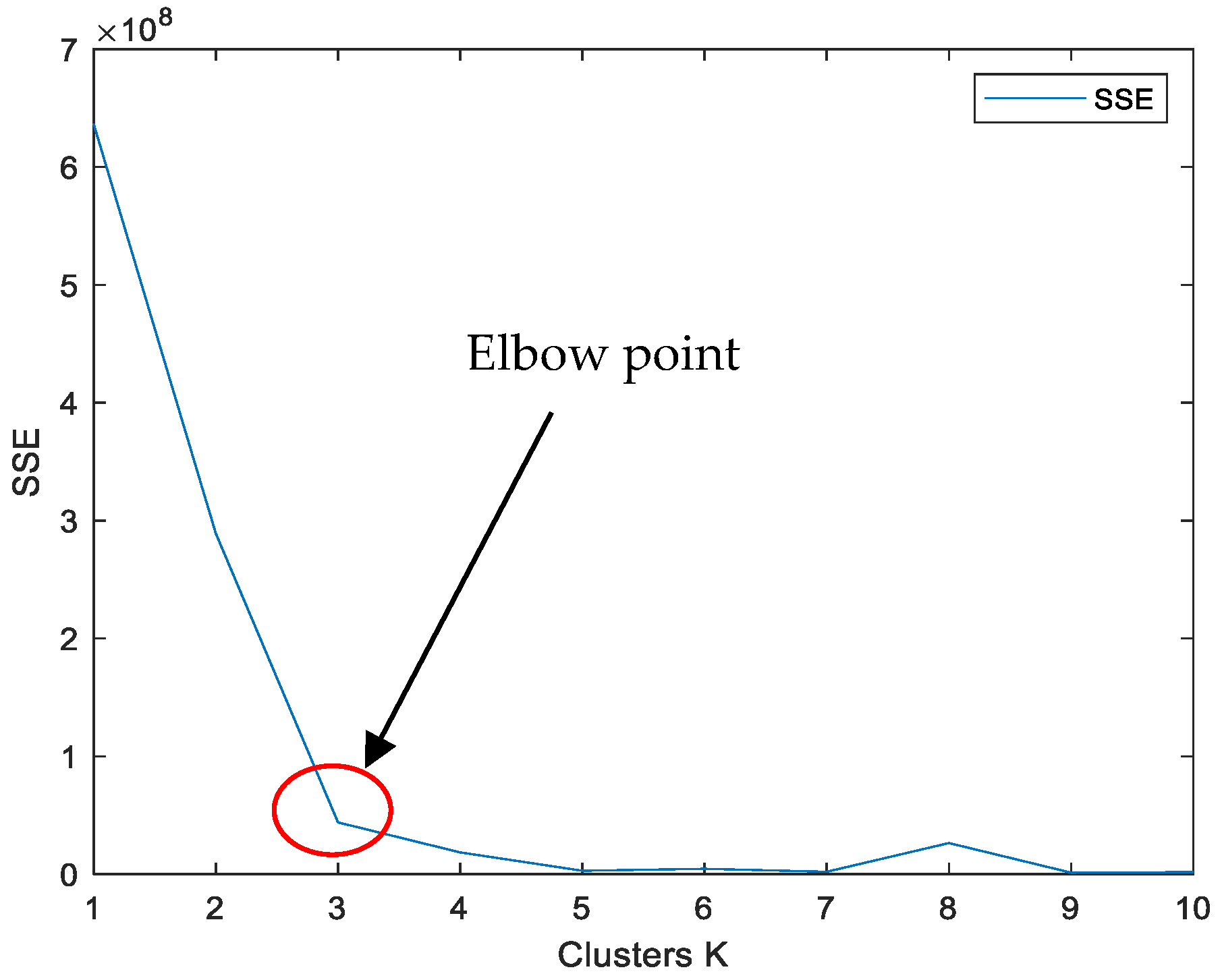
Apply the Elbow method to the K-means clustering method to find the optimal initial number of clusters and reduce the computational time.
Solve the POPF for a variable load of a weekend day in summer using the GTO.
The following portions of this paper are arranged:
Section 2 presents the problem formulation, the POPF, and its restrictions and penalty terms.
Section 3 introduces the mathematical models of the RESs. The Monte Carlo Simulation method combined with the K-means clustering method and the Elbow method is introduced in
Section 4.
Section 5 offers the Artificial Gorilla Troops optimization algorithm. The simulation results from the suggested optimization technique applied to the standard IEEE 30- and 118-bus systems are shown in
Section 6, along with a comparison study on several optimization techniques reported in this paper. Finally,
Section 7 concludes the whole study.
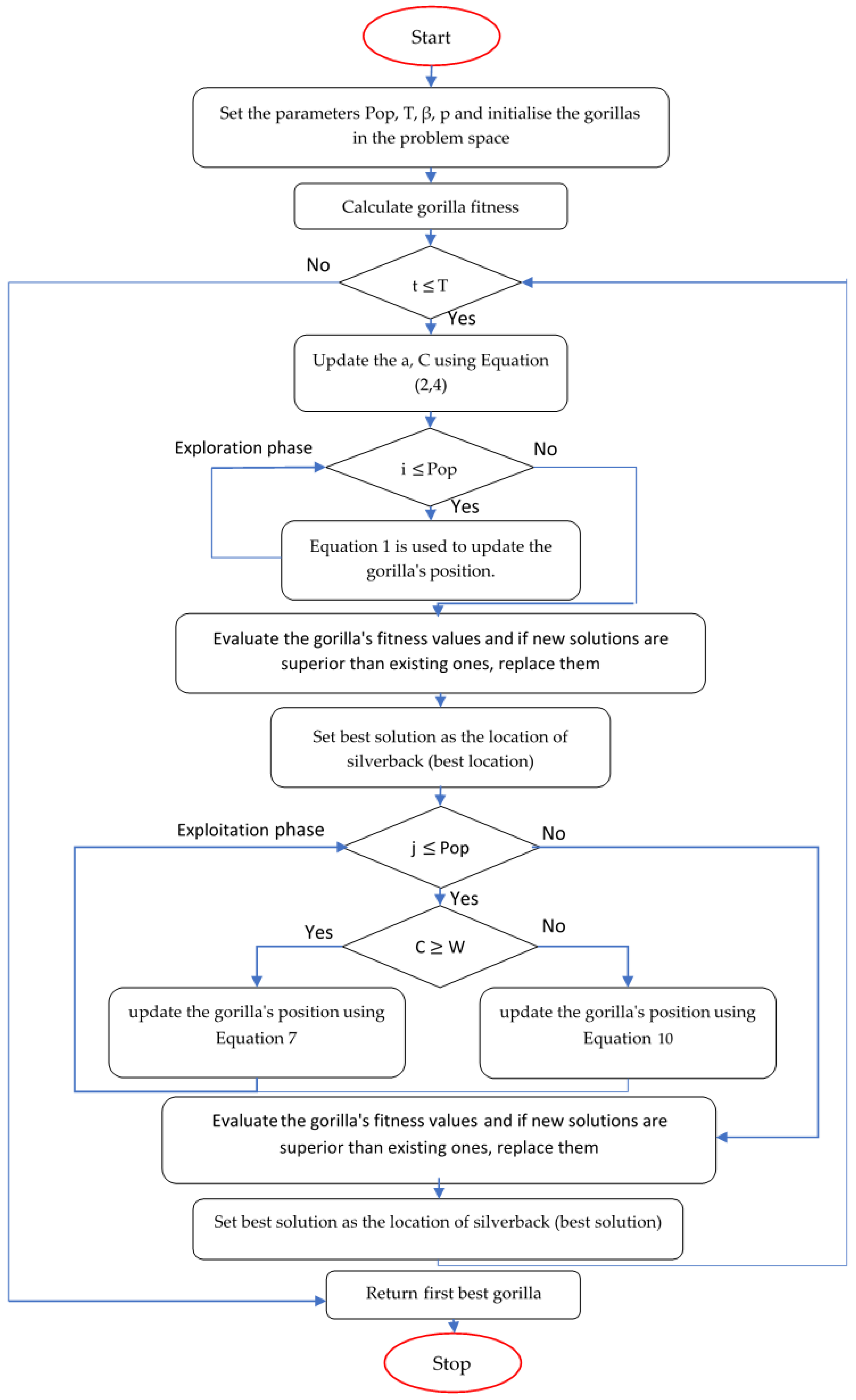
6. Simulation Results and Discussion
This paper proposed a solution for the OPF and POPF issues by applying the GTO algorithm. To verify the viability and performance of the suggested GTO-based OPF and POPF problem, the IEEE 30-bus and 118-bus systems were applied.
Table 3 lists the details of these two power systems [
36]. The effectiveness of the suggested algorithm is compared with GA (Genetic Algorithm) [
57], PSO (Particle Swarm Optimization) [
58], SFO (Sunflower Optimization) [
59], HHO (Novel Harris Hawk Optimization) [
60], and HFPSO (Hybrid Firefly Particle Swarm Optimization) [
61] for a classical OPF. Algorithms used as competitors were the HHO and SFO for the POPF, including renewable energy. The control parameter of the OPF issue wasre the active power output from the thermal generators. The iteration number was selected to achieve good performance for the suggested GTO technique.
The selection of the controlling parameter of the GTO method was such as any metaheuristic optimization technique. The trial-and-error method was used to choose these parameters with many independent trials and finally to check the algorithm’s performance. Many various cases have been shown to demonstrate the efficacy of the proposed algorithm. All scenarios were ran for fixed and variable loads. The fixed load is the standard load for the standard test systems mentioned in this paper. The variable load is the load of an available summer weekday and is presented in [
62].
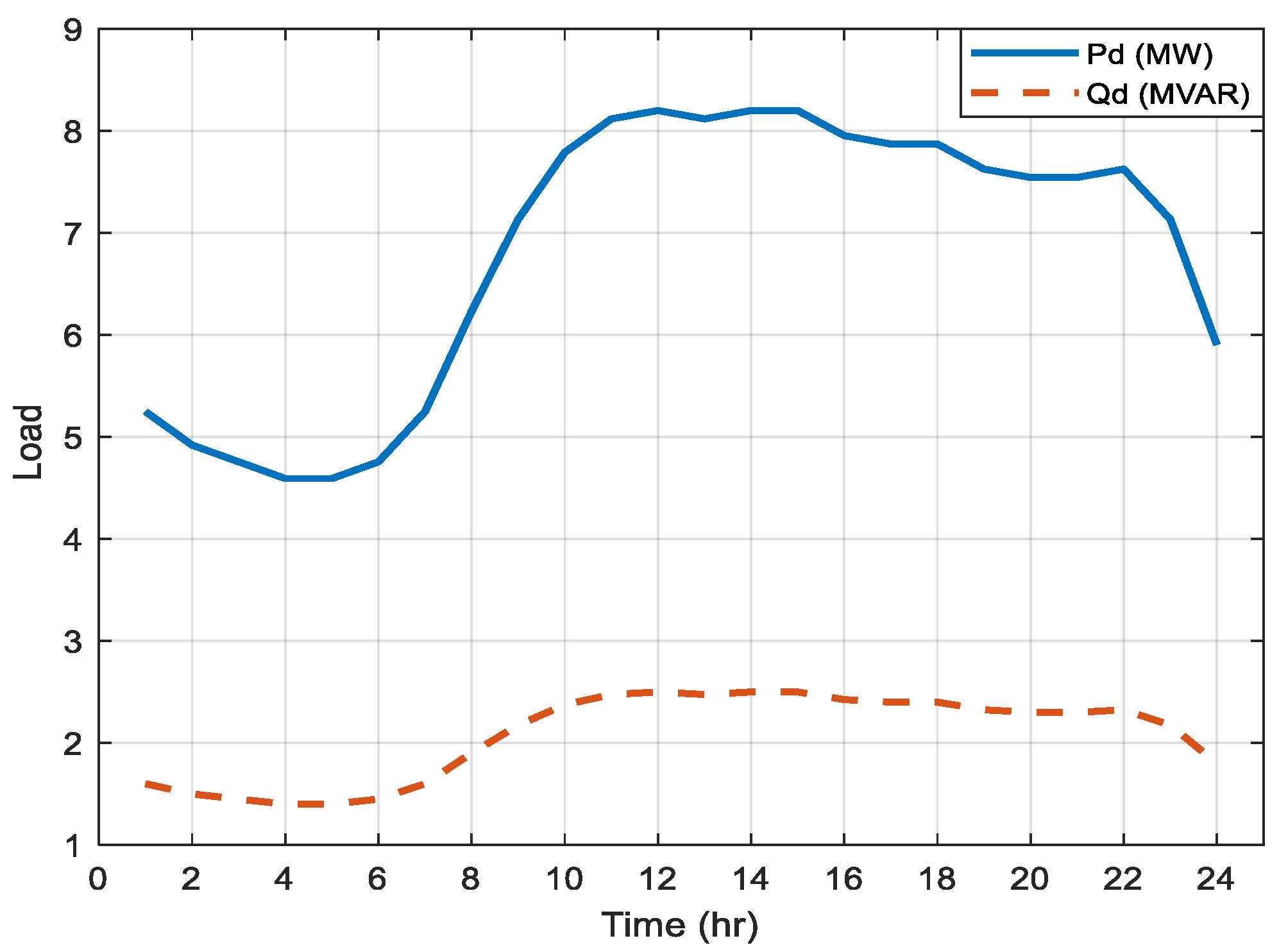
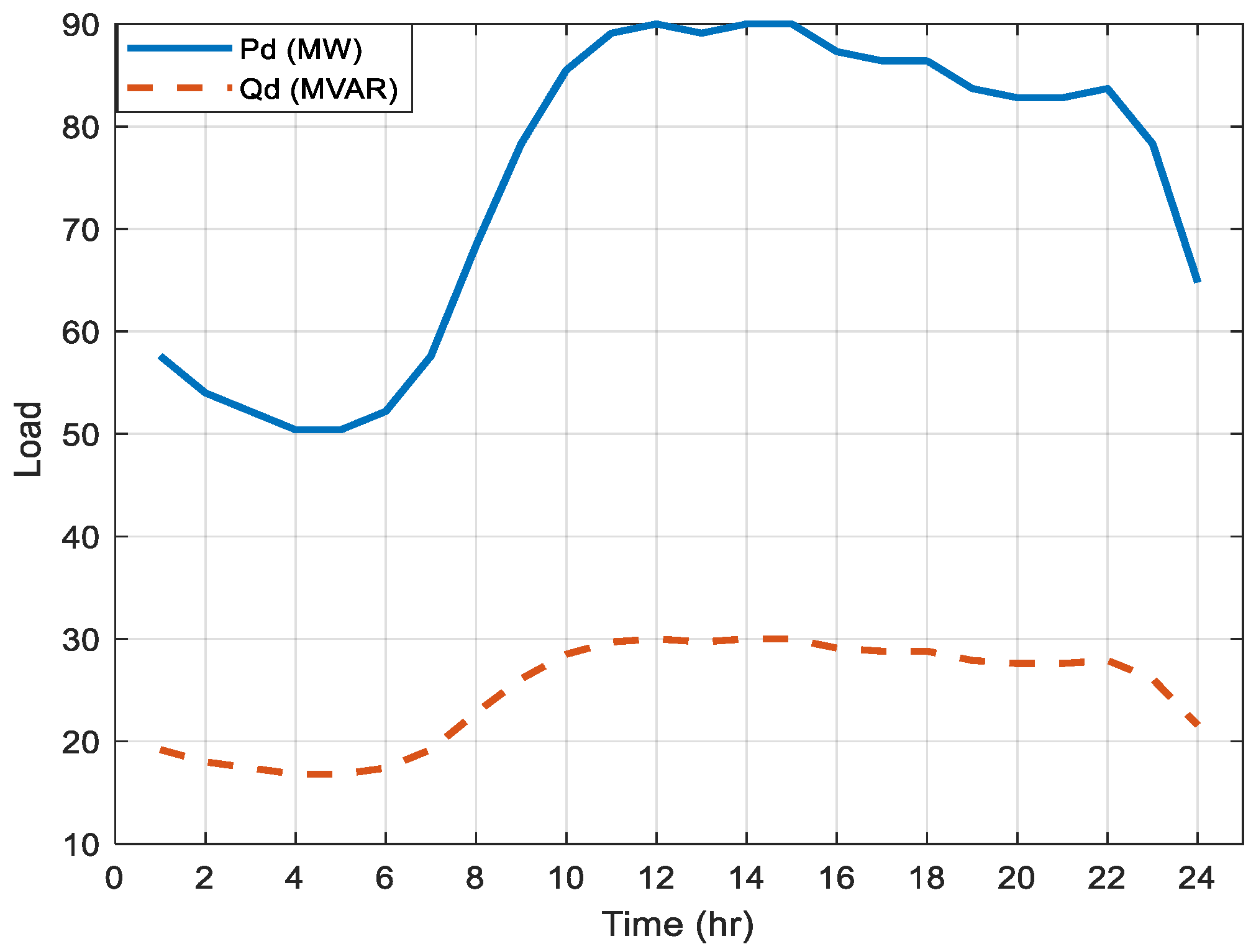
Figure 10 and
Figure 11 show an example of the variable load curve over a summer day at bus 15 for the IEEE 30-bus and IEEE 118 systems, respectively. To prove the efficacy of the proposed approach for OPF and POPF problems, three different scenarios were considered, as are shown in
Table 4. The performance and efficacy of the proposed GTO algorithm have been confirmed by comparison with the other chosen approaches.
6.1. The IEEE 30-Bus System
The small-scale power system was used to verify the proposed algorithm’s performance. The classical OPF problem with no RESs and the POPF with PV & wind generators at the optimal bus locations were solved. The results were compared to those from other algorithms reported in this paper to confirm their viability. Finally, the proposed algorithm was used to investigate how adding PV and wind generators would affect the system’s overall operating costs.
6.1.1. Case 1: Classical OPF
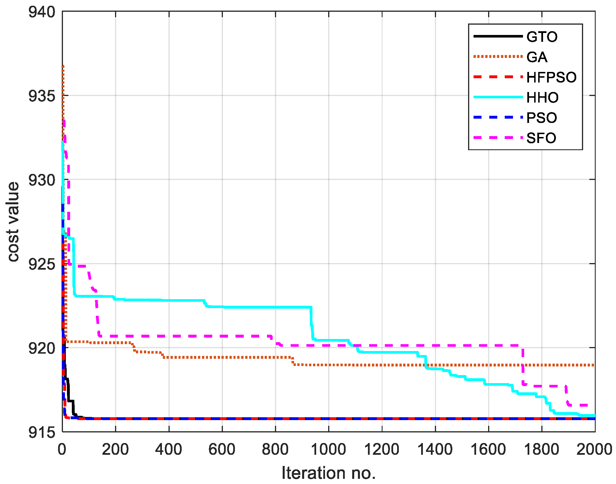
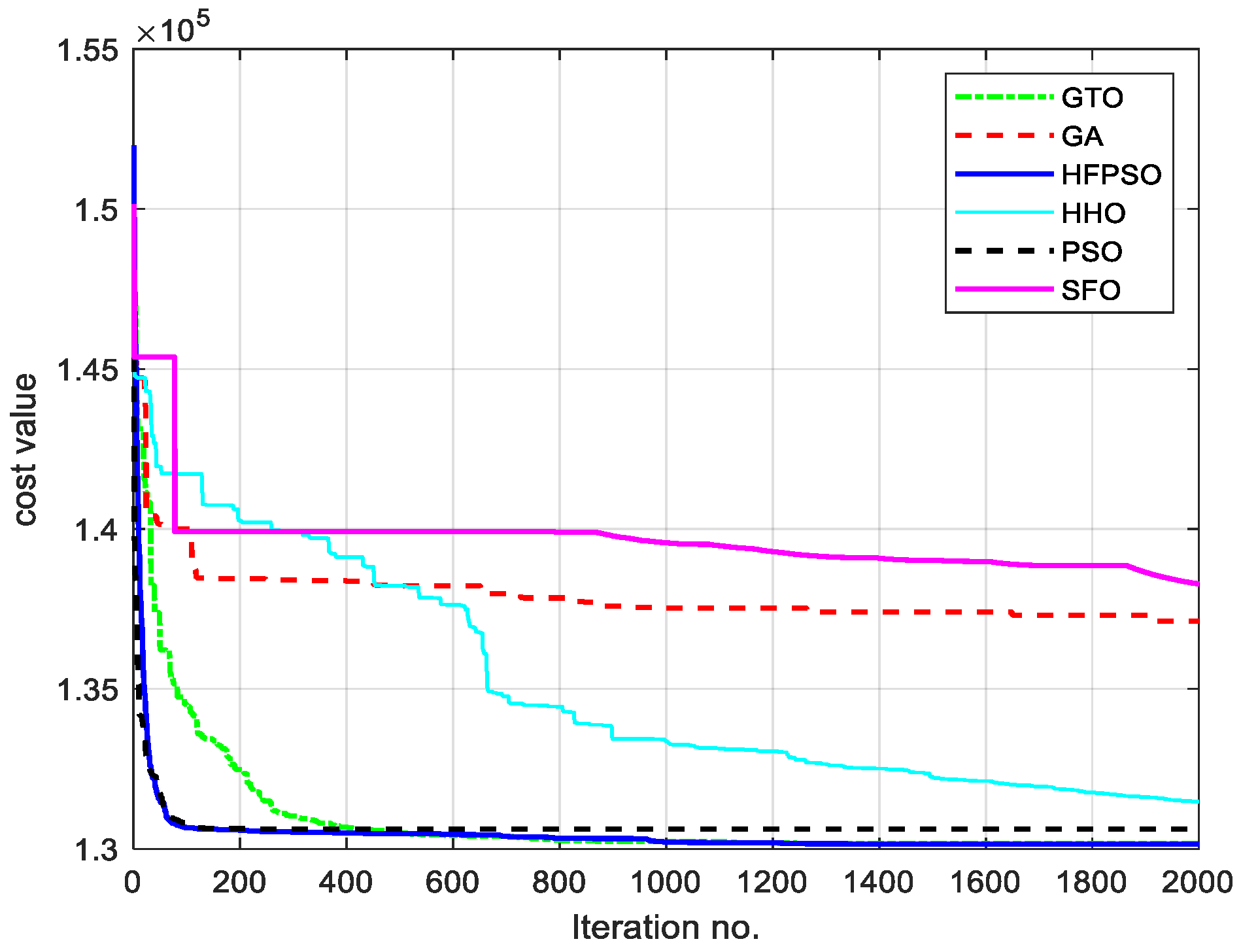
In this case, the proposed technique was used for solving the classical OPF with the fixed load. Its results were then compared to the GA, PSO, SFO, HHO, and HFPSO to verify the performance of the suggested technique. The objective function was to reduce the thermal generator’s cost function with no renewable energy added to the system. For all algorithms, the sizes of the population were set at 30. The number of iterations for all algorithms was set at 2000. The optimized control variables and the objective function calculated by GTO are compared to the results from other algorithms in
Table 5.
Figure 12 shows a comparison of the conversion curve of the objective function for the different algorithms. It is clear from
Figure 12 that the GTO outperforms the other techniques in finding the minimum cost with fewer iterations.
6.1.2. Case 2: POPF with RESs
In this case, the PV and wind generators were inserted into the optimal bus locations [
64], as is shown in
Table 6. The rating of the added PV and wind generators were 20 MW and 30 MW, respectively, and were selected such that the total capacity of the RESs represented 17.6% of the total load of the IEEE 30-bus systems. The sizes of the population for all algorithms were set as 15. The number of iterations for all algorithms was set at 200. The proposed technique was used for solving the POPF for fixed and variable loads. The suggested approach’s results were then compared to the other chosen algorithms such as the PSO and HHO. The time-varying load is shown in
Figure 10 for the standard 30-bus system. Due to changes in irradiance and wind speed, the active power production from the wind and PV generators varied. Therefore, the RESs’ uncertainty was considered when forecasting the RESs’ output power.
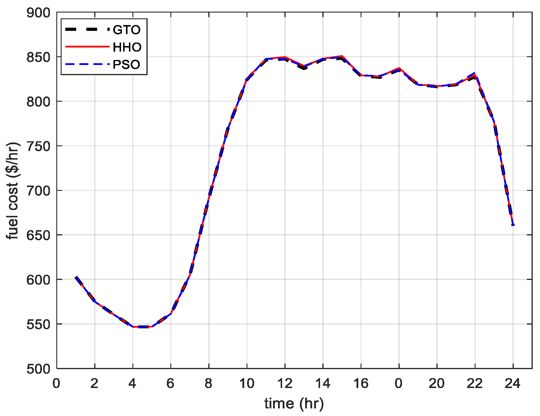
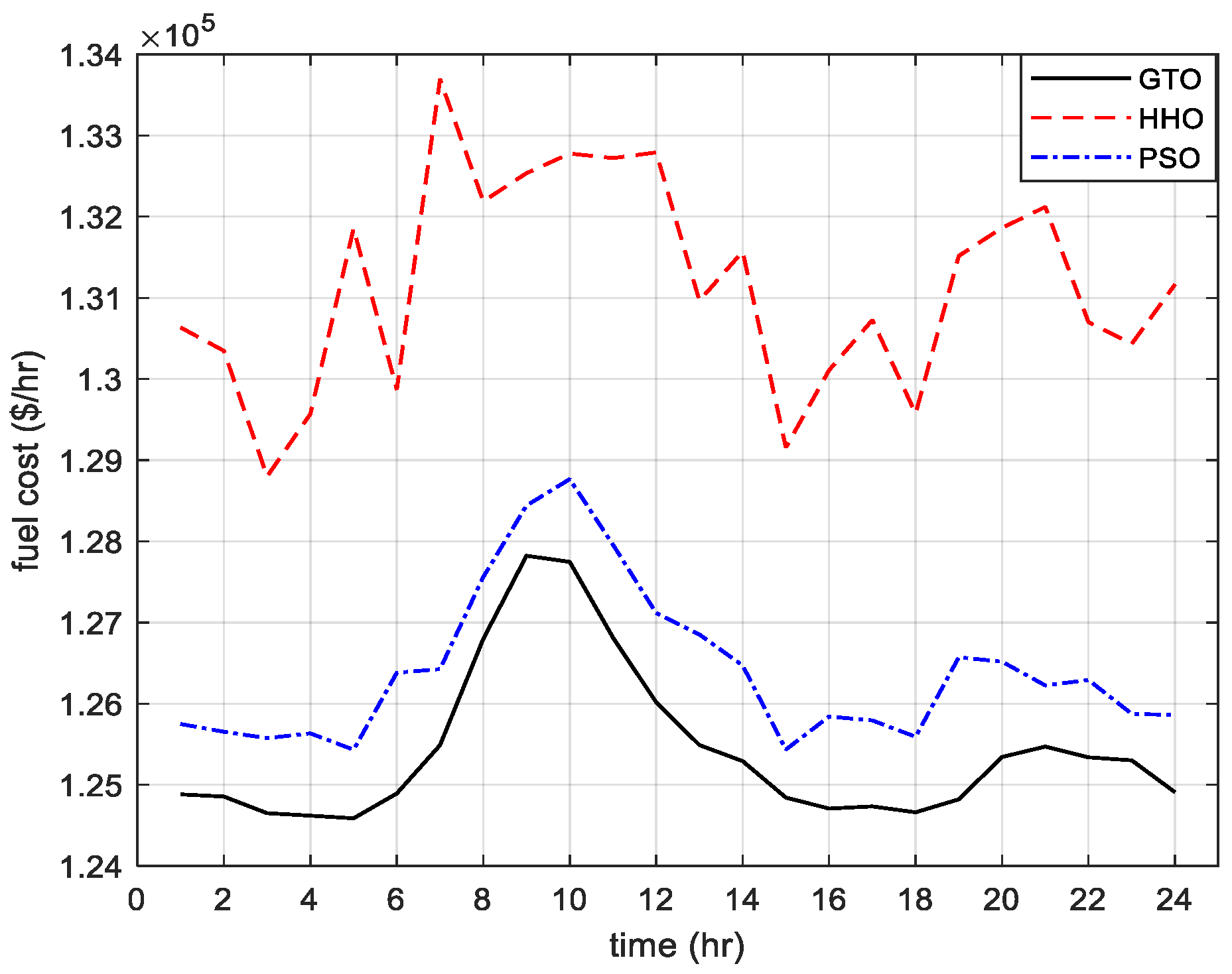
Figure 13 and
Figure 14 show the convergence of the objective function for the proposed GTO algorithm against the HHO and PSO techniques under fixed and variable loading, respectively. The results indicated that the fuel cost calculated by the GTO is relatively less than the other two algorithms for fixed and variable loads. The results from the proposed approach are significantly superior to results from the other algorithms for fixed load, but for a variable load the results are very similar.
6.1.3. Case 3: Effects of Adding the RES on the Total Cost
After confirming that the suggested algorithm successfully founds the optimal results for either the classical OPF or the POPF, the effect of adding the RESs on the system’s total operating cost was considered. The proposed algorithm was used for solving the POPF problem considering the uncertainties of the RESs for fixed and time-varying loads. The ratings of the PV, rating of the wind generators, population size, and the number of iterations were kept the same as in the previous case study.
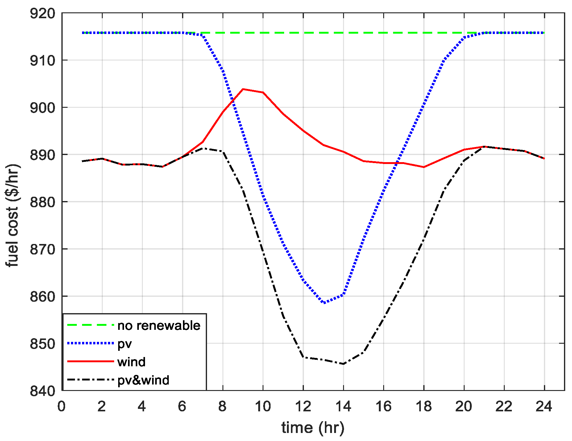
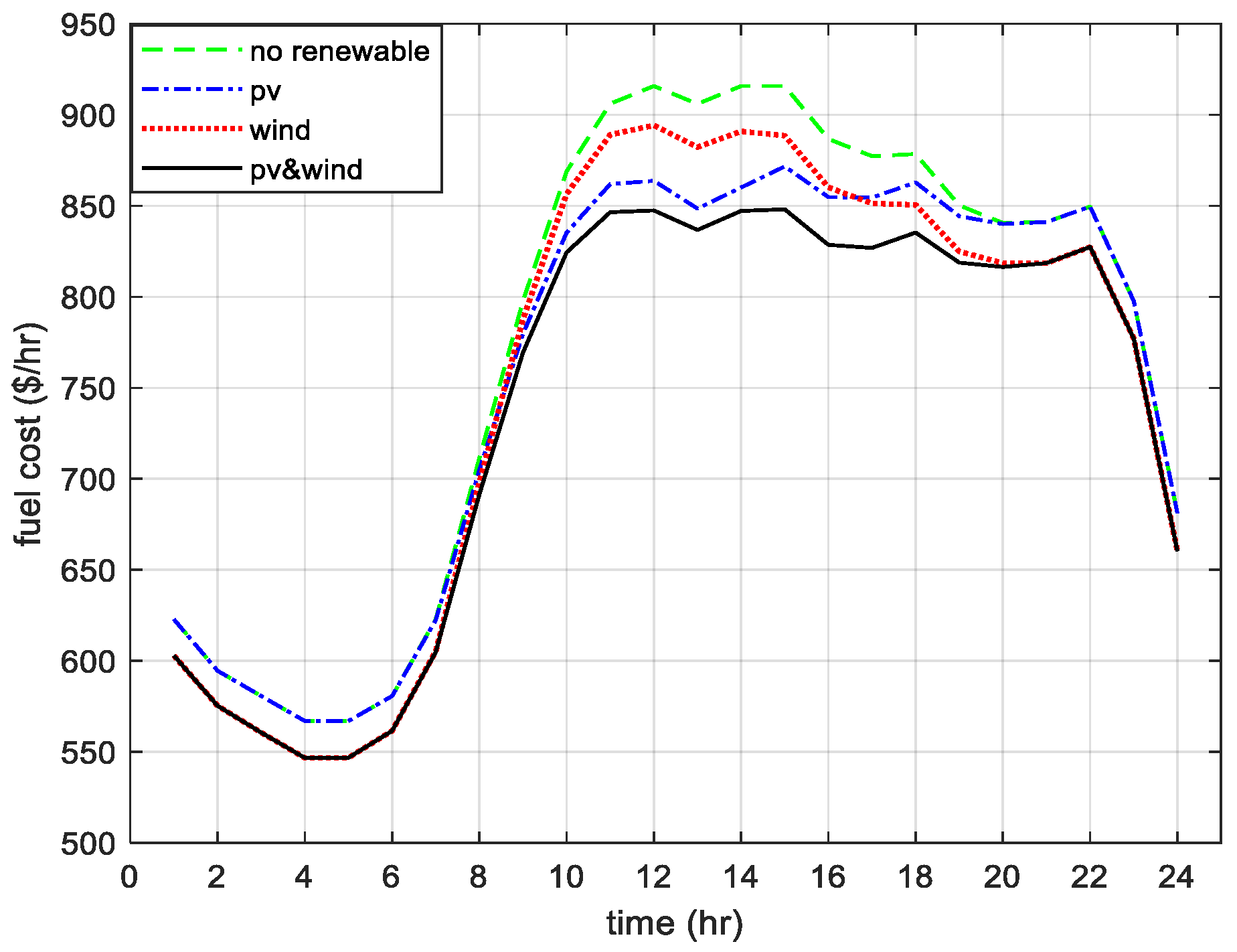
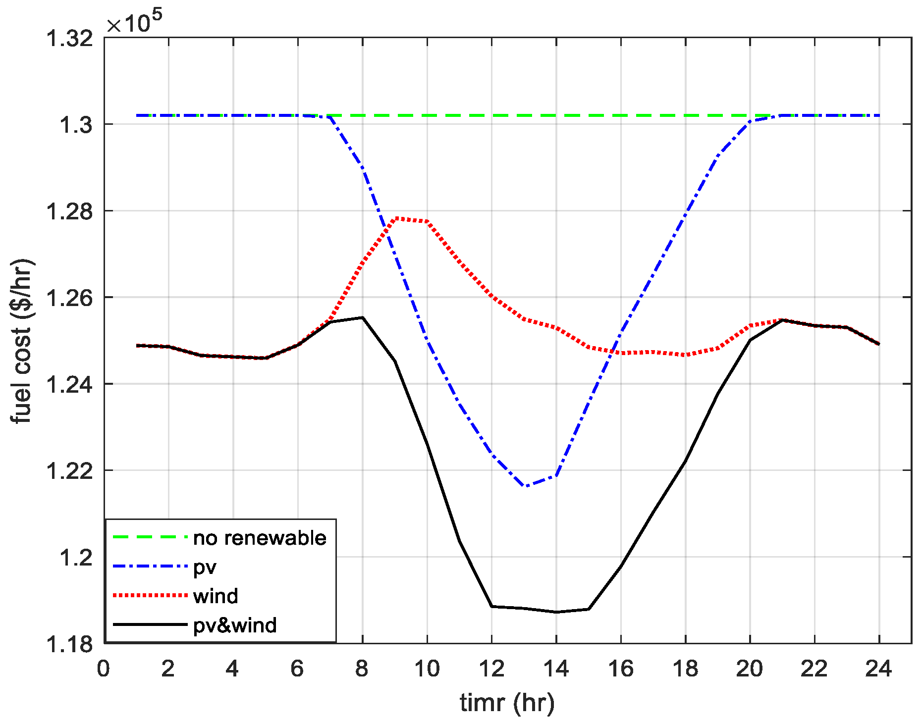
Figure 15 and
Figure 16 show the effect of adding the RESs to the optimal bus locations on the system’s total operating cost. For the fixed and variable loads, adding the PV generators to the system reduced the total cost from hour 7 to hour 20 (as the solar irradiance existed only during this period), while adding the wind generators reduced the total cost throughout the day. Extreme cost reduction occurred when adding both PV and wind generators simultaneously.
Table 7 and
Table 8 summarize the cost reduction percentage from adding PV and wind generators for each hour during the equivalent summer day with fixed and time variable loads, respectively.
6.2. The IEEE 118-Bus System
The proposed algorithm’s performance was evaluated using the large-scale power system. The classical OPF with no RESs and the POPF with PV and wind generators at the optimal bus locations were solved. The results of the suggested approach were compared with those of the other selected algorithms to confirm its viability. Then, the proposed algorithm was used to study the effect of inserting the PV and wind generators on the system’s total operating cost.
6.2.1. Case 4: Classical OPF
The proposed approach was used for solving the classical OPF with the fixed load and then comparing its results with the GA, PSO, SFO, HHO, and HFPSO methods to verify the effectiveness of the suggested technique. The objective function was to reduce the thermal generator’s cost function with no renewable energy added to the system. The sizes of the population for all algorithms were set at 30. The number of iterations in all algorithms was set as 2000. The best results of the control variables and the objective function calculated by GTO are compared to the results from other algorithms in
Table 9.
Figure 17 compares the conversion curve of the objective function for the different algorithms. Comparing other algorithms verified that the GTO algorithm is capable of finding a more advantageous solution.
6.2.2. Case 5: POPF with RESs
In this case, the PV and wind generators were inserted into the optimal bus locations [
64], as is shown in
Table 6. The rating of the added PV and wind generators were 250 MW and 500 MW, respectively. The total capacity of the RESs represents 17.6% of the total system load, such that the percentage of penetration of the RESs was kept the same for the standard 30-bus and 118-bus systems. The sizes of the population for all algorithms were set at
30. The number of iterations for all algorithms was set at
400. The proposed approach was used to solve the POPF, including the RESs, to minimize the fuel cost for fixed and variable loads and to compare the suggested approach with the other chosen algorithms, such as PSO and HHO. The time-varying load is shown in
Figure 11 for the standard 118-bus system.
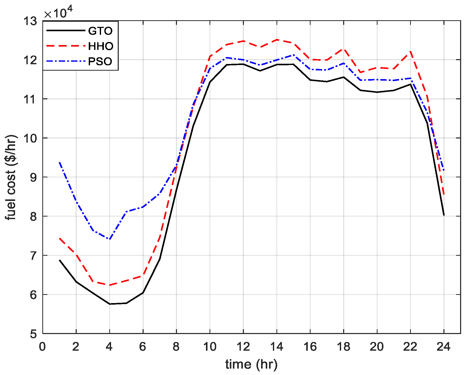
Figure 18 and
Figure 19 show the convergence curves of the objective function under fixed and variable loading, respectively. The results indicated that the fuel cost calculated by the GTO was less than the other two algorithms for fixed and variable loads, respectively. The results from the proposed approach were significantly superior to results from the other chosen algorithms mentioned in the literature for both fixed and variable loading conditions.
6.2.3. Case 6: Effects of Adding RESs on the Total Cost
After confirming the performance of the suggested approach in finding the optimal solution, whether for classical OPF or POPF in the large-scale system, the effect of adding the RESs on the overall system cost was considered. The proposed approach was used for solving the POPF problem considering the uncertainties of the RESs for fixed and time-varying loads. The ratings of PV generators, wind generators, the size of the population, and the number of iterations were kept the same as in the previous case studies.
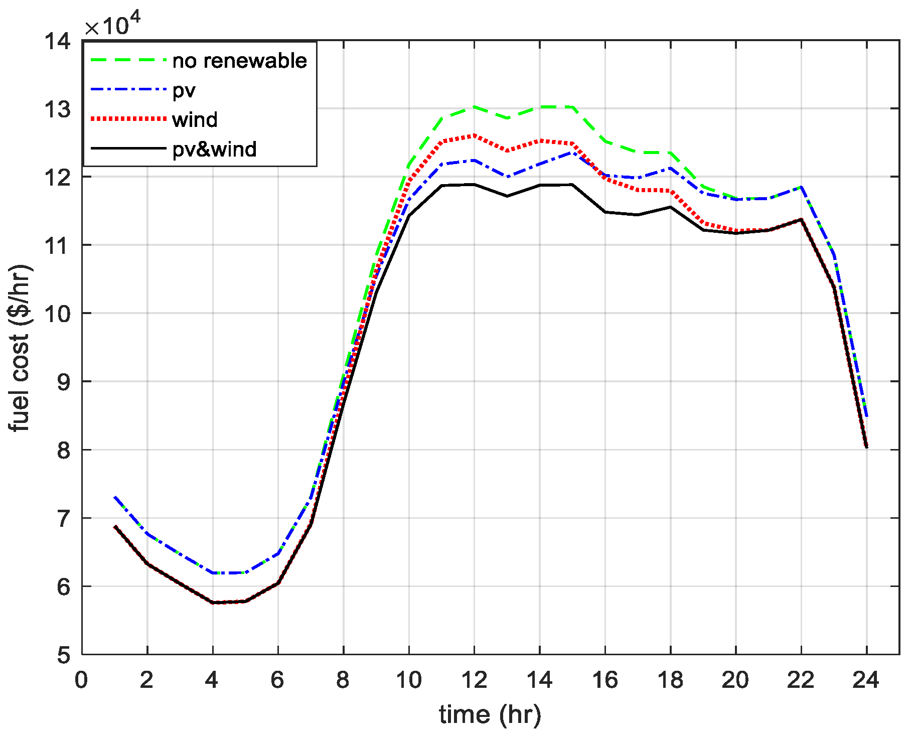
Figure 20 and
Figure 21 show how adding the RESs to the optimal bus locations affects the overall system cost. For the fixed and variable loads, adding the PV generators to the system reduces the total cost from hour 7 to hour 20, as solar irradiance exists only during this period. Adding the wind generators reduces the total cost all over the day, and extreme cost reduction occurs when adding both PV and wind generators simultaneously.
Table 10 and
Table 11 show the cost reduction percentages from adding PV and wind generators for each hour during the equivalent summer day with fixed and variable time loads, respectively. The percentage reduction can be higher for higher RES penetration levels. These reductions happened when only 17.6% of DGs were inserted.

 ,
, 


