Sustainable Supply Chain System for Defective Products with Different Carbon Emission Strategies

Abstract

Many nations have created ecological policies and regulations to prevent industries from emitting excessive amounts of carbon emissions into the environment. While significant progress has been achieved in the direction of sustainable growth, many nations still rely on nonrenewable energy sources. This study explores the viability of investing in green technology to achieve the optimal decisions (lot sizes, lead time, and green investment amount) in a two-echelon supply chain system by considering human error with two carbon emission strategies: carbon taxes and limited carbon emissions. It entails the inspection of every shipped lot by the buyer to identify defective products that could have resulted from the vendor’s production process. We show a constrained non-linear program and design a calculus-optimization technique to solve it. The methodology used in this research is the quantitative method, which is based on the principles of operations research, and the models are built on mathematically oriented inventory theory. The results imply that an outsized ecological carbon footprint can be reduced without compromising customer service by designing optimal inventory strategies. The findings also confirm that green investment is the greatest economical method for reducing carbon emissions and system costs.

1. Introduction

The normal practice in a multinational venture is to have an integrated sustainable supply chain (SC) system, which is beneficial for both producer and buyer. The entire production–distribution inventory system generates carbon at every stage. Increased human habits have led to a rise in greenhouse gases in the air over the last 150 years. The biggest cause of carbon emitted into the atmosphere is the burning of fossil fuels for power, warmth, and transport. Burning fossil fuels for power and the greenhouse gases produced by the chemical processes that make things from raw materials are the principal sources of carbon pollution from industry. The greatest security threat that contemporary humanity has ever faced in the current century is climate change. The leading contributor to climate change caused by humans is greenhouse gases (GHG), mainly carbon emission. All industries must consider the necessity of reducing carbon emission in order to combat climate change and implement the Paris Agreement. It’s crucial for a manufacturing business to understand where carbon emissions occur and what variables have the most impact on carbon emission, if it wants to minimize them. Carbon emissions from industry can be reduced by appropriate managerial decisions, economical inventory control, high-potential technologies, and energy-efficient warehousing. In view of this, today there are a lot of disputes for governments and firms.

The carbon regulatory authorities in different industrialized countries have adopted different policies to lower the emissions from industries. The main policies are limited carbon emissions and carbon taxation, which are often adopted by governments. One more policy exists in some countries such as the USA, China, etc., called carbon cap and trade, which is not discussed in this paper. In this scheme, companies will be taxed if they produce a higher level of carbon emissions than their permitted allowances. Limited carbon emissions and carbon taxation policies have been implemented in many developing and developed countries. However, pursuing a reduction in carbon emissions regardless of economic growth is not practical for developing countries. Instead, most developing countries would have to face a tradeoff between environmental protection and economic growth. As a result, this study focuses on inventory strategy in an SC, while taking into account the two distinct carbon emission regulations described above. Most relevant research previously studied this topic from the perspective of a single firm, without considering human error and inventory lead time, which cannot achieve overall SC optimization. This study, thus, offers an integrated approach from the perspectives of both ends of an SC with carbon emission, human error, and variable lead time concern, which is the major difference from the related studies in the literature.

1.1. Literature Review

Trade parties develop a strategic alliance to maximize profit and decrease costs, while exchanging information to achieve greater advantages. Numerous authors have recently explored an integrated SC system in various problem situations (see [1,2,3]). Das et al. [4] discussed the random credit period within their model. The manufacturer offered extra time for retailers to pay. Nezamoddini et al. [5] illustrated an artificial neural network and genetic algorithm for the optimization of risk-based SC management. Priyan and Mala [6] developed an inventory policy for pharmaceutical products. They found a game approach for the quality degradation of perishable products. Product quality has quickly become a crucial competitive factor. Buying businesses frequently conduct inspections to guarantee that external raw materials and products are of excellent quality [7]. Although new technologies are being created that may help with quality-appraisal mechanization, most companies still depend on human supervisors. One of the most important elements impacting logistics efficiency and inventory systems is human error. The operator may classify the industrial batches as perfect or imperfect.

Khan et al. [7] documented an inventory system for defective commodities and the human errors that occurred during the inspection. Priyan and Uthayakumar [8] designed mathematical models and techniques for handling two-stage multi-constraints inventory issues with quality-review flaws. Zhou et al. [9] examined a model for synergic economic order quantity with scarcities, trade credits, flawed condition, and verification errors. Khan et al. [10] addressed inspection error and defective products in the SC by assuming that the buyer has the choice of having the faulty items repaired by a local producer or getting new items locally to replace them. Taheri et al. [11] derived a model for faulty goods, preventative maintenance, inspection errors, and partial backlogging in uncertain situations. Tiwari et al. [12] studied the influence of human errors on an SC model. Feng et al. [13] developed joint economic lot-size problem models that include faulty items, where the producer is in authority of the production process and inspection and reworking procedures. Wakhid [14] provided a mathematical model for an inventory system in a closed-loop SC system made of a producer and many sellers. In contrast to the aforementioned papers, Subhajit et al. [15] used control theory to solve an imperfect production problem in an interval ecosystem by a carbon-emission-investment approach.

Lead time is another issue with inventory interaction between buyers and sellers. When the SC is caused by uncertain demand, the reduction in lead time and backorder price discounts becomes substantial. Liao and Shyu [16] examined the varying lead times. They suggested an inventory model using the assumption entailing the possibility of breaking down the lead time into various linear parts, which differ in their linear continuity with regards to crashing costs, whereby the crashing costs component may be reduced by the consideration of a normally distributed lead-time demand. Another study by Pan and Yang [17] was based on the idea that the seller would reduce the lead time if the consumer requested it. Hoque [18] studied the impact of batch sizes and shorter lead times on stock renewal methods in the supplier–purchaser relationship. Modak and Kelle [19] mentioned an SC where the customer can shop online or at DFA-derived shops. On the other hand, Priyan and Mala [6] proposed a healthcare SC model that considers different quality traits for raw materials and completed products as well as lead-time and service-level constraints.

Over the last few years, the literature on carbon emissions in the inventory system has exploded. Benjaafar et al. [20] wrote one of the leading papers in this field. Hammami et al. [21] created an inventory model with regulation for the carbon tax and cap. Li et al. [22] described the creation of two optimal models for SC systems that included carbon emissions. Tang et al. [23] derived the (R, Q) inventory policy for lowering the emissions and inventory management in the transportation industry. Halat and Hafezalkoto [24] used a game-theory technique to study the cause of harmonization, the control of emissions and costs, and the empirical responsibility of governments. Huang et al. [25] examined carbon policies and green technologies on the SC by considering carbon emission during product production, transportation, and storage. Trade-credit policy (Tiwari et al., [26]) and fuzzy decision-making (Yadegaridehkordi et al., [27]) are both contributions to the development of sustainability. Later, several authors (see [28,29,30,31]) worked on emissions and the carbon footprint to reduce the carbon in the ecosystem. Yuqiang et al. [31] proposed an emission cap and trade system to limit carbon emissions.

Table 1. Review of the literature.

Author(s)	Multi-Echelon Model	Human Error	Carbon Emission	Green Investment	Limited Carbon Emission and Carbon Taxation	Controllable Lead Time
Khanra et al. [3]	✓
Das et al. [4]	✓
Priyan and Mala [6]	✓					✓
Priyan and Uthayakumar [8]	✓	✓
Khan et al. [10]	✓	✓
Taheri-Tolgari et al. [11]	✓	✓
Tiwari et al. [12]	✓	✓
Pan and Yang [17]	✓					✓
Hoque [18]	✓					✓
Hammami et al. [21]			✓	✓	✓
Li et al. [22]	✓		✓		✓
Tang et al. [23]			✓
Halat and Hafezalkoto [24]	✓		✓
Huang et al. [25]	✓		✓	✓	✓
Yang et al. [28]			✓	✓
Md. Rakibul [29]			✓	✓	✓
Biswajit et al. [30]	✓		✓		✓
Yuqiang et al. [31]	✓		✓
This paper	✓	✓	✓	✓	✓	✓

offers the relative similarities and differences to compare some of the previous works with this study.

As can be seen in Table 1, most of the studies did not take all the important aspects into consideration. The major contribution of this study to the literature is that the proposed integrated model deals with the inventory management for both sides of the SC, regarding the two carbon emissions policies and green investment. Carbon emissions can be from the processes of production, delivery, and storage, and the investment in green technology is expected to reduce such carbon emissions. Based on the above discussions, the objective of this study is to minimize the total related costs in the SC by setting the optimal delivery quantity, number of deliveries, lead time, and amount of green investment under the two different carbon emissions policies.

1.2. Research Motivations and Contributions

Small errors can quickly escalate into major catastrophes. The Mars Climate Orbiter destroyed a USD 327.6 million spacecraft due to a measurement conversion error [32]. Ask any manufacturer how a counting error, or a misread label forced them to shut down an entire production line. According to a study by Vanson Bourne, manufacturers realize the agony of accidental downtime caused by human error better than any other industry. The study added that human error is responsible for 23% of all unexpected downtime in production. This compares to an average of 9% in other industries including oil and gas, energy, medicine, and logistics. The report also claims that almost half of manufacturers (45%) recognize that there is space for improvement when it comes to preventing asset concerns in their company. According to reports, 82% have experienced unanticipated downtime at least once in the last three years [32]. A DOE report’s main finding is that a range of circumstances outside the control of front-line personnel impacts behavior and results. Human errors in production are becoming more obvious every day as technology progresses. Human error accounts for more than 80% of all failures and faults [33].

Scrap items due to human errors and imperfect production traders will become more important than ever as the planet’s resources come to an end and the risk of climate change forces power conservation. The generation of waste is rising constantly, creating a large opportunity for recycling, which protects power and reduces GHG emissions. The Environment Directorate of the Organization for Economic Co-operation and Development (OECD) said that “the paucity of virgin materials may soon become a concern” [34]. According to the OECD, annual source extraction will climb to 80 billion tons by 2020, roughly twice what it was in 2002, and 100 billion tons by 2030. This presents a significant potential for the recycling business, but it also represents a major difficulty. According to research conducted by Imperial College London, recycling trash saves 354,000 tons of carbon dioxide, one of the major GHG, per 100,000 tons of aluminum generated. “The 500,000 tons or more of GHG emissions avoided via recycling are worth $40 or more per ton,” Nicholas Stern, the author of fundamental climate change research, stated [34]. The recycling industry already saves the equivalent of 1.8% of global fossil fuel emissions. The author added that the recycling business saves nearly as much energy as the aviation industry.

Keeping the benefits of recycling in mind, the implications of green technology and human error on a complex SC system, by examining two emission options, carbon taxes and limited carbon emissions, have been explored in this article. This paper involves combining research streams such as controllable lead time, an integrated two-echelon SC model, green investment in different carbon emission policies, and human error in inspection into one research frame. Therefore, this study entails an integrated production inventory, considering human errors and carbon emissions. The assumption is that carbon emissions result from production, transportation, and storage. From this assumption and a model setting, the following questions are answered: (1) What would be the industry’s economic inventory strategy if lead time demand is unpredictable under various carbon emission policies? (2) To reduce carbon emissions, what would be the exact green investment? (3) What are the consequences of misclassification errors on decision-making?

The rest of the article is organized as follows: Notations and assumptions are listed in Section 2. Section 3 contains the mathematical formulations of the inventory issue as well as the solution process. The topic of sensitivity and numerical analysis is found in Section 4. The summary of the paper is discussed in Section 5.

2. Notation and Assumptions

The subsequent terminology is utilized for this proposed study.

Assumptions

(i)

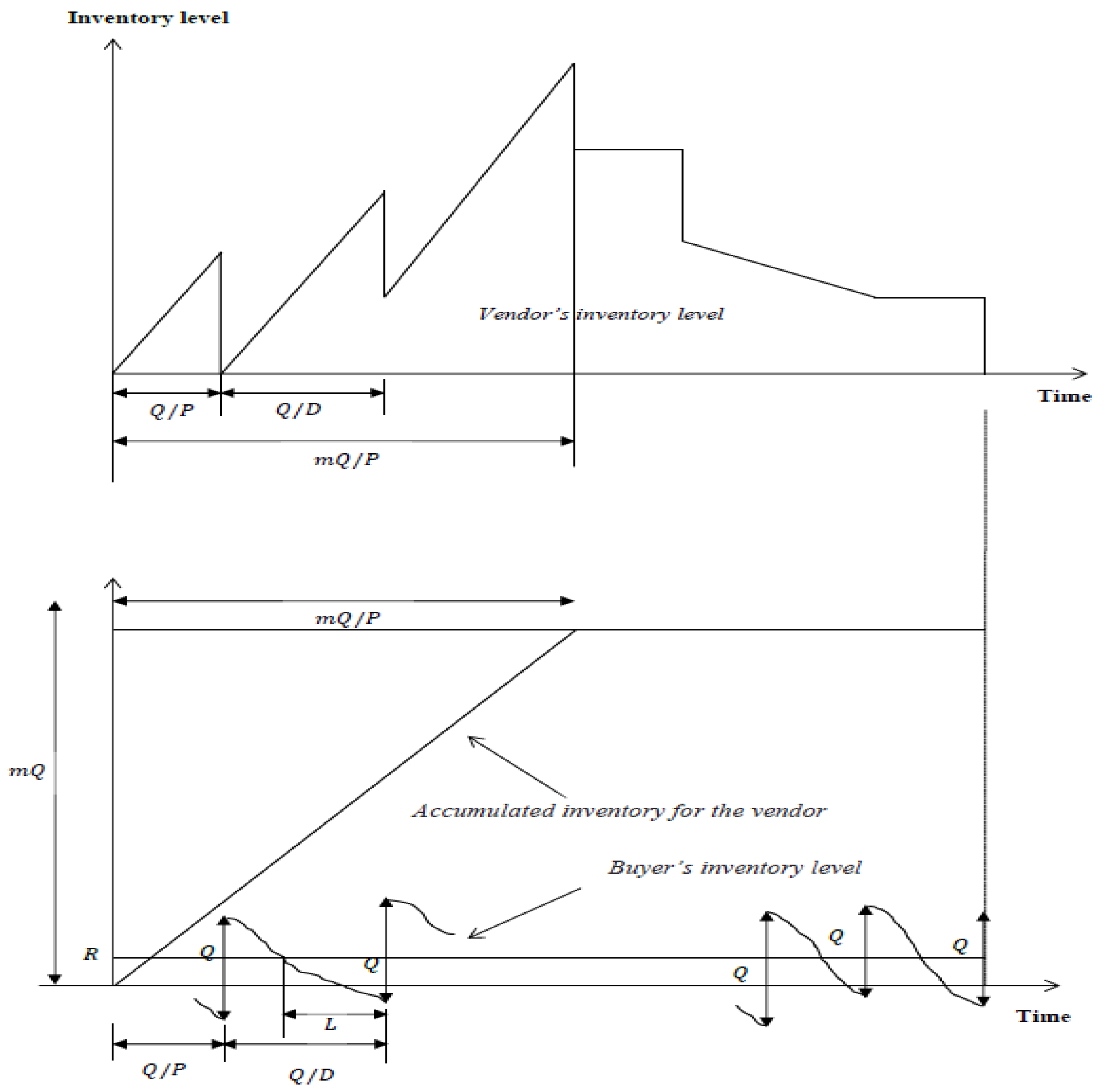
A single form of an item is used for the production–inventory model. The buyer can place order Q to be shipped in n number of equal-sized deliveries once the inventory reaches r.

(ii)

The lead-time demand X follows a normal probability distribution function $f_X \left(x\right)$, with mean $DL$ and standard deviation $\sigma \surd L$. The r is defined as r $=DL+k\sigma \surd L$, where $k$ signifies the safety component. The L comprises m jointly autonomous modules, whereby the ith module has a normal period $b_i$, a least period $a_i$, and a crashing cost $u_i$. These are rearranged conveniently to give $u_i$, such that $u_1<u_2<\cdots <u_m$. $L$ constituents are crashed at some point in time, beginning with the first element due to its lowest unit-crashing cost, followed by the next element, and then the subsequent elements afterwards.

(iii)

Let $L_0={\displaystyle \sum }_{i=1}^m{b}_i,$ and $L_i$ be the span of $L$ with modules $1,2,\cdots ,i$ crashed to their lowest period; then $L_i$ can be stated as $L_i=L_0-{\displaystyle \sum }_{j=1}^i\left(b_j-a_j\right), i=1,2,\cdots m;$ and the crashing cost for $L$ per cycle is B $B\left(L\right)=u_i\left(L_{i-1}-L\right)+{\displaystyle \sum }_{j=1}^{i-1}{u}_j\left(b_j-a_j\right), L\in \left[L_i,L_{i-1}\right]$.

(iv)

The manufacturing sector produces defective items due to use of a long-run system. Thus, after a certain time, this system starts to produce defective items. The fraction of faulty items is found in all lots, and, thus, all lots are immediately screened at a constant rate $s_r$, which is higher than $D$.

(v)

Carbon emissions arise in the process of manufacturing, transportation, and storage. To reduce emissions from the system, additional investment is used. According to Huang et al. [25], to reduce carbon emissions, investment in green technology can be utilized. The green technology function for reducing emissions is presented as $R\left(G\right)=\alpha G-\beta G^2$.

3. Model Development

The vendor delivers the products to the buyer, who places an order of $Q$ units, which are received as n number of shipments. Every lot delivered has y percentage of defective items. Therefore, the buyer does an inspection for each received lot upon arrival of each shipment at a given continuous screening rate of $s_r$, to remove faulty commodities. Nevertheless, during the buyer-verification process, two forms of error (Type I and Type II) can occur. Type I happens when products that are not faulty are classified as faulty products, while Type II occurs when faulty products are classified as non-faulty items. Hence, the fraction of faulty products identified by assessors are given as $y_e=p_1\left(1-y\right)+y\left(1-p_2\right)$, where $\left(1-y\right)p_1$ and $\left(1-p_2\right)y$ are the respective fractions for Type II and Type I screening errors.

The inspection process and the faulty rate are naturally random, and, therefore, it is considered that $y$, $p_1$, and $p_2$ are random independent variables. Hence, the buyer’s expected value of an observed imperfect item is $E\left[y_e\right]=\left(1-E\left[y\right]\right)E\left[p\right]+E\left[y\right]\left(1-E\left[p_2\right]\right)$(Tiwari et al., 2020). Simply, it is notified by $E\left[y_e\right]$ as $y_e$. Therefore, the order-cycle length of the buyer is $\frac{Q\left(1-Y_e\right)}{D}$.

3.1. Model without Considering Carbon Emissions

3.1.1. Modeling for Buyer

The buyer continuously assesses its inventory, and when it reaches $r$, the buyer places an order of $Q$ units, which is received in $n$ number of deliveries by the vendor. Shortages happen when $X>r$. Consequently, at the end of the cycle, the buyer’s expected shortages are derived by $E{\left(X-r\right)}^{+}={\displaystyle {{\displaystyle \int }}_r^{\infty }}\left(x-r\right)f_x\left(x\right)=\sigma \sqrt{L}\Psi \left(k\right)$, where $\Psi \left(k\right)=\phi \left(k\right)-k\left[1-\Phi \left(k\right)\right]>0; \phi \mathrm{and} \Phi$ are p.d.f. and c.d.f., respectively. Hence, the expected back-order quantity is given by $\gamma \sigma \sqrt{L}\mathsf{\Psi }\left(k\right)$. The expected loss of sale is $\left(1-\gamma \right)\sigma \sqrt{L}\mathsf{\Psi }\left(k\right)$, and the shortage cost is $\left[{\pi }_x\gamma +{\pi }_0\left(1-\gamma \right)\right]\sigma \sqrt{L}\mathsf{\Psi }\left(k\right)$ per cycle. Therefore, over the given cycle, the expected faulty inventory items are $\frac{Q\left(1-Y_e\right)}{2}+\mathrm{safety}\mathrm{stock}+\mathrm{previous}\mathrm{cycle}\mathrm{lost}\mathrm{sale}$. Thus, the cost of non-faulty and faulty goods per unit of time for the customer’s aggregate holding cost is $h_b\left[\frac{Q\left(1-Y_e\right)}{2}+\frac{DQ{Y}_e}{s_r\left(1-Y_e\right)}+k\sigma \sqrt{L}+\left(1-\gamma \right)\sigma \sqrt{L}\mathsf{\Psi }\left(k\right)\right]$.

Some miscalculation costs are incurred by the buyer because of errors in inspection, and these are the costs for the falsely accepted faulty products and the non-faulty items that are falsely rejected. The cost for miscalculation of a Type I error, which is the cost of incorrectly banned perfect commodities, is ${\mu }_{0}Q\left(1-E\left[y\right]\right)E\left[p_1\right]$, whereas the miscalculation cost for a type II error, which is the cost of incorrectly acknowledged perfect commodities, is $\mu QE\left[y\right]E\left[p_2\right]$. Henceforth, the cost of aggregate miscalculation per unit of time is designed by $\frac{D}{1-Y_e}\left[\mu E\left[y\right]E\left[p_2\right]+{\mu }_0\left(1-E\left[y\right]\right)E\right[p_1]$. Also, the number of faulty items that are found correctly is $QE\left[y\right](1-E\left[p_2\right]$. Hence, the buyer’s cost for scraping is $\frac{C_{0}D}{1-Y_e}E\left[y\right]\left(1-E\left[p_2\right]\right)$.

The aggregate expected cost for the customer represents the summation of misclassification, holding, screening, ordering, and backorder costs. That is,

$$\begin{array}{ll}T{C}_B\left(Q,L\right)& =\frac{AD}{\left(1-Y_e\right)Q}+h_b\left[\frac{\left(1-Y_e\right)Q}{2}+\frac{DQ{Y}_e}{s_r\left(1-Y_e\right)}+k\sigma \sqrt{L}+\left(1-\gamma \right)\sigma \sqrt{L}\mathsf{\Psi }\left(k\right)\right]\\ & +\frac{D}{Q\left(1-Y_e\right)}\left[{\pi }_x\gamma +{\pi }_0\left(1-\gamma \right)\right]\sigma \sqrt{L}\mathsf{\Psi }\left(k\right)+\frac{\mu D}{1-Y_e}E\left[y\right]E\left[p_2\right]+\frac{{\mu }_{0}D}{1-Y_e}\left(1-E\left[y\right]\right)E\left[p_1\right]\hfill \\ & +\frac{C_{s}D}{1-Y_e}+\frac{DB\left(L\right)}{\left(1-Y_e\right)Q}+\frac{C_{0}D}{1-Y_e}E\left[y\right]\left(1-E\left[p_2\right]\right)\end{array}$$

3.1.2. Modeling for Vendor

The setup cost per unit of time for the vendor is $\frac{SD}{nQ\left(1-Y_e\right)}$. Here, $F$ is the unit transport cost, and $d$ is the delivery distance. Then, the vendor’s yearly transportation cost is $\frac{D}{Q\left(1-Y_e\right)}Fd$.

On the other hand, the average inventory for a vendor is the difference between the accumulated inventories of the vendors and buyers (Figure 1), i.e., $\frac{D}{nQ}\left[\left\{nQ\left(\frac{Q}{P}+\frac{Q}{D}\left(n-1\right)\right)-\frac{n^2{Q}^2}{2p}\right\}-\left\{\frac{Q^2}{D}\left(1+2+3+\dots +\left(n-1\right)\right)\right\}\right]=\frac{Q}{2}\left[\left(n-1\right)-\frac{D}{P}\left(n-2\right)\right]$.

Hence, the vendor’s holding cost is $\frac{h_{v}Q}{2\left(1-Y_e\right)}\left[\left(n-1\right)-\frac{D}{P}\left(n-2\right)\right]$. The joint expected total inventory cost is $ETC\left(Q,n,L\right)=T{C}_B\left(Q,L\right)+T{C}_V\left(Q,n\right)$. It is mathematically expressed as:

$$\begin{array}{ll}JETC\left(Q,n,L\right)& =\frac{AD}{Q\left(1-Y_e\right)}+h_b\left[\frac{Q\left(1-Y_e\right)}{2}+\frac{DQ{Y}_e}{s_r\left(1-Y_e\right)}+k\sigma \sqrt{L}+\left(1-\gamma \right)\sigma \sqrt{L}\mathsf{\Psi }\left(k\right)\right]\\ & +\frac{D}{Q\left(1-Y_e\right)}\left[{\pi }_x\gamma +{\pi }_0\left(1-\gamma \right)\sigma \sqrt{L}\mathsf{\Psi }\left(k\right)\right]+\frac{\mu D}{1-Y_e}E\left[y\right]E\left[p_2\right]+\frac{{\mu }_{0}D}{1-Y_e}\left(1-E\left[y\right]\right)E\left[p_1\right]\\ & +\frac{C_{s}D}{1-Y_e}+\frac{DB\left(L\right)}{\left(1-Y_e\right)Q}+\frac{C_{0}D}{1-Y_e}E\left[y\right]\left(1-E\left[p_2\right]\right)+\frac{SD}{\left(1-Y_e\right)nQ}+\frac{D}{Q\left(1-Y_e\right)}Fd\\ & +\frac{h_{v}Q}{2\left(1-Y_e\right)}\left[\left(n-1\right)-\left(n-2\right)\frac{D}{P}\right]\end{array}$$

3.2. Carbon Emission Policies with Green Investments

Here, $P$ is the constant production rate, $E_P$ and $E_S$ are the emissions from the production of a unit of product and the setup of the production cycle, respectively. Then, each year, the emissions from the production process are $D{E}_P+\frac{D}{nQ\left(1-Y_e\right)}{E}_S$. Here, $E_T$ is the carbon emission from transporting a vehicle at a unit distance.

Therefore, the carbon emission from transportation is $\frac{D}{Q\left(1-Y_e\right)}{E}_{T}d$. Now, $E_h$ is the carbon emission from storing a unit of product for both the buyer and vendor.

Hence, the yearly carbon emissions from holding products by the buyer and vendor are $E_h\left[\frac{Q\left(1-Y_e\right)}{2}+\frac{DQ{Y}_e}{s_r\left(1-Y_e\right)}+k\sigma \sqrt{L}+\left(1-\gamma \right)\sigma \sqrt{L}\mathsf{\Psi }\left(k\right)+\frac{Q}{2\left(1-Y_e\right)}\left\{\left(n-1\right)-\left(n-2\right)\frac{D}{P}\right\}\right]$.

It is assumed that green technology can be invested to reduce emissions. By Assumption 5, $R\left(G\right)=\alpha G-\beta G^2$ is the green cost in the SC investment. Consequently, the joint predictable total inventory cost of the system and the amount of carbon emissions are given by

$$\begin{array}{ll}JETC\left(Q,n,L,G\right)& =\frac{AD}{Q\left(1-Y_e\right)}+h_b\left[\frac{Q\left(1-Y_e\right)}{2}+\frac{DQ{Y}_e}{s_r\left(1-Y_e\right)}+k\sigma \sqrt{L}+\left(1-\gamma \right)\sigma \sqrt{L}\mathsf{\Psi }\left(k\right)\right]\\ & +\frac{D}{Q\left(1-Y_e\right)}\left[{\pi }_x\gamma +{\pi }_0\left(1-\gamma \right)\right]\sigma \sqrt{L}\mathsf{\Psi }\left(k\right)+\frac{\mu D}{1-Y_e}E\left[y\right]E\left[p_2\right]+\frac{{\mu }_{0}D}{1-Y_e}\left(1-E\left[y\right]\right)E\left[p_1\right]\\ & +\frac{C_{s}D}{1-Y_e}+\frac{DB\left(L\right)}{Q(1-Y_{e)}}+\frac{C_{0}D}{1-Y_e}E\left[y\right]\left(1-E\left[p_2\right]\right)+\frac{SD}{nQ\left(1-Y_e\right)}+\frac{D}{Q\left(1-Y_e\right)}Fd\\ & +\frac{h_{v}Q}{2\left(1-Y_e\right)}\left[\left(n-1\right)-\left(n-2\right)\frac{D}{P}\right]+G\end{array}$$

and

$$E\left(Q,n,L,G\right)=D{E}_P+\frac{D}{nQ\left(1-Y_e\right)}(E_S+n{E}_{T}d)-\left(\alpha G-\beta G^2\right)$$

$$+E_h\left[\frac{Q\left(1-Y_e\right)}{2}+\frac{DQ{Y}_e}{s_r\left(1-Y_e\right)}+k\sigma \sqrt{L}+\left(1-\gamma \right)\sigma \sqrt{L}\mathsf{\Psi }\left(k\right)+\frac{Q}{2\left(1-Y_e\right)}\left\{\left(n-1\right)-\left(n-2\right)\frac{D}{P}\right\}\right]$$

respectively.

3.2.1. Carbon Taxation

The carbon tax is indicated as $C_t$ from the unit emissions. Both parties are willing to invest in green technology and a carbon price to reduce emissions. Therefore, the integrated expected total cost for this scenario is the sum of the buyer’s ordering cost, the vendor’s production setup cost, the product’s transport cost, both parties’ holding costs, a carbon tax for the holding inventory for both parties’ carbon tax for production setup, a carbon tax for the production process, the buyer’s backorder cost, a misclassification cost, a screening cost, a crashing cost, a scrapping cost, and the green cost minus the emissions reduction efficiency.

This is mathematically expressed as

$$JET{C}_t\left(Q,n, L,G\right)=\frac{D}{nQ\left(1-Y_e\right)}\left[nA+S+C_t{E}_s\right]+\frac{D}{Q\left(1-Y_e\right)}\left[F+C_t{E}_T\right]d$$

$$\begin{gathered} +\left(h_b+C_t{E}_h\right)\left[\frac{Q\left(1-Y_e\right)}{2}+\frac{DQ{Y}_e}{s_r\left(1-Y_e\right)}+k\sigma \sqrt{L}+\left(1-\gamma \right)\sigma \sqrt{L}\mathsf{\Psi }\left(k\right)\right] \\ \hspace{1em}\hspace{1em}\hspace{1em}\hspace{1em}\hspace{1em}\hspace{1em}+\left(h_v+C_t{E}_h\right)\frac{Q}{2\left(1-Y_e\right)}\left\{\left(n-1\right)-\left(n-2\right)\frac{D}{P}\right\}+C_{t}D{E}_P \end{gathered}$$

$$\begin{gathered} +\frac{D}{Q\left(1-Y_e\right)}\left[{\pi }_x\gamma +{\pi }_0\left(1-\gamma \right)\right]\sigma \sqrt{L}\mathsf{\Psi }\left(k\right)+\frac{\mu D}{1-Y_e}E\left[y\right]E\left[p_2\right]+\frac{{\mu }_{0}D}{1-Y_e}\left(1-E\left[y\right]\right)E\left[p_1\right]+\frac{C_{s}D}{1-Y_e} \\ +\frac{DB\left(L\right)}{Q(1-Y_{e)}}+\frac{C_{0}D}{1-Y_e}E\left[y\right]\left(1-E\left[p_2\right]\right)-C_t\left(\alpha G-\beta G^2\right)+G \left(1\right) \end{gathered}$$

(1)

Lemma 1: 

For fixed $n$, $L$, and $G$, $JET{C}_t\left(Q,n,L,G\right)$ is convex in $Q$.

Proof. 

Evaluating the first- and second-order derivatives of $JET{C}_t\left(Q,n,L,G\right)$ with respect to

(w.r.t) $Q$, we obtain

$$\frac{\partial JET{C}_t\left(Q,n,L,G\right)}{\partial Q}=-\frac{D}{n{Q}^2\left(1-Y_e\right)}\left[nA+S+C_t{E}_s\right]-\frac{D}{Q^2\left(1-Y_e\right)}\left[F+C_t{E}_T\right]d$$

$$+\left(h_b+C_t{E}_h\right)\left[\frac{\left(1-Y_e\right)}{2}+\frac{D{Y}_e}{s_r\left(1-Y_e\right)}\right]+\left(h_v+C_t{E}_h\right)\frac{1}{2\left(1-Y_e\right)}\left\{\left(n-1\right)-\left(n-2\right)\frac{D}{P}\right\}$$

$$-\frac{D}{Q^2\left(1-Y_e\right)}\left[{\pi }_x\gamma +{\pi }_0\left(1-\gamma \right)\right]\sigma \sqrt{L}\mathsf{\Psi }\left(k\right)-\frac{DB\left(L\right)}{Q^2\left(1-Y_e\right)}$$

(2)

and

$$\frac{{\partial }^{2}JET{C}_t\left(Q,n,L,G\right)}{\partial Q^2}=\frac{2D}{n{Q}^3\left(1-Y_e\right)}\left[nA+S+C_t{E}_s\right]+\frac{2D}{Q^3\left(1-Y_e\right)}\left[F+C_t{E}_T\right]d$$

$$+\frac{2D}{Q^3\left(1-Y_e\right)}\left[{\pi }_x\gamma +{\pi }_0\left(1-\gamma \right)\sigma \sqrt{L}\mathsf{\Psi }\left(k\right)\right]+\frac{2DB\left(L\right)}{Q^3\left(1-Y_e\right)}>0$$

Therefore, for a fixed value of $n$, $L$, and $G$, $JET{C}_t\left(Q,n,L,G\right)$ is convex in $Q$. $⯀$

Result 1: For a fixed $n$ and $G$, Equation (2) is set to zero, and the subsequent optimal $Q_t$ for the buyer is found.

$$Q_t^{*}={\left\{\frac{\frac{D}{\left(1-Y_e\right)}\left[A+\frac{1}{n}\left(S+C_t{E}_s\right)+d\left(F+C_t{E}_T\right)+\left[{\pi }_x\gamma +{\pi }_0\left(1-\gamma \right)\right]\sigma \sqrt{L}\mathsf{\Psi }\left(k\right)+B\left(L\right)\right]}{\left(h_b+C_t{E}_h\right)\left[\frac{1-Y_e}{2}+\frac{D{Y}_e}{s_r\left(1-Y_e\right)}\right]+\left(h_v+C_t{E}_h\right)\frac{1}{2\left(1-Y_e\right)}\left[\left(n-1\right)-\left(n-2\right)\frac{D}{P}\right]}\right\}}^{\frac{1}{2}}$$

(3)

Lemma 2: 

For fixed $Q$, $L$, and $G$, $JET{C}_t\left(Q,n,L,G\right)$ is convex in $n$.

Proof. 

Evaluating the first- and second-order derivatives of $JET{C}_t\left(Q,n,L,G\right)$ w. r. t. $n$, we obtain

$$\frac{\partial JET{C}_t\left(Q,n,L,G\right)}{\partial n}=-\frac{D}{Q{n}^2\left(1-Y_e\right)}\left[S+C_t{E}_s\right]+\left(h_v+C_t{E}_h\right)\frac{Q}{2\left(1-Y_e\right)}\left(1-\frac{D}{P}\right)$$

and

$$\frac{{\partial }^{2}JET{C}_t\left(Q,n,L,G\right)}{\partial n^2}=\frac{2D}{Q{n}^3\left(1-Y_e\right)}\left[S+C_t{E}_s\right]>0$$

Hence, for the fixed value of $Q$, $L$, and $G$, $JET{C}_t\left(Q,n,L,G\right)$ is convex in $n$. $⯀$

Lemma 3: 

For fixed $Q$, $n$, and $L$, $JET{C}_t\left(Q,n,L,G\right)$ is convex in $G$.

Proof. 

Evaluating the first- and second-order derivatives of $JET{C}_t\left(Q,n,L,G\right)$ w. r. t. $G$,

$$\frac{\partial JET{C}_t\left(Q,n,L,G\right)}{\partial G}=1-C_t\left(\alpha -2\beta G\right)$$

(4)

and

$$\frac{{\partial }^{2}JET{C}_t\left(Q,n,L,G\right)}{\partial G^2}=2\beta C_t>0$$

Thus, for fixed $Q$,$n$ and $L$, $JET{C}_t\left(Q,n,L,G\right)$ is convex in $G$.$⯀$

Result 2: Equating (4) to zero gives the optimal amount of green investment

$$G_t^{*}=\frac{1}{2}\left[\frac{\alpha }{\beta }-\frac{1}{C_t\beta }\right]$$

(5)

Lemma 4: 

For fixed $Q$, $n$, and $G$, $JET{C}_t\left(Q,n,L,G\right)$ is concave in $L$.

Proof. 

Evaluating the first- and second-order derivatives of $JET{C}_t\left(Q,n,L,G\right)$ w. r. t. $L$,

$$\frac{\partial JET{C}_t\left(Q,n,L,G\right)}{\partial L}=\frac{D{B}^{\prime }\left(L\right)}{Q\left(1-Y_e\right)}+\left\{\left(h_b+C_t{E}_h\right)\left(k\sigma +(1-\gamma \right)\sigma \mathsf{\Psi }\left(k\right))+\frac{D}{Q\left(1-Y_e\right)}\left[{\pi }_x\gamma +{\pi }_0\left(1-\gamma \right)\right]\sigma \mathsf{\Psi }\left(k\right)\right\}\frac{1}{2\sqrt{L}}$$

and

$$\frac{{\partial }^{2}JET{C}_t\left(Q,n,L,G\right)}{\partial L^2}=\frac{D{B}^{″}\left(L\right)}{Q\left(1-Y_e\right)}$$

$$+\left\{\left(h_b+C_t{E}_h\right)\left(k\sigma +(1-\gamma \right)\sigma \mathsf{\Psi }\left(k\right))+\frac{D}{Q\left(1-Y_e\right)}\left[{\pi }_x\gamma +{\pi }_0\left(1-\gamma \right)\right]\sigma \mathsf{\Psi }\left(k\right)\right\}\left(\frac{-1}{4L^{\frac{3}{2}}}\right)<0$$

Thus, for the fixed value of $Q$,$n$ and $G$, the $JET{C}_t\left(Q,n,L,G\right)$ is concave in $L$.$⯀$

Result 3: According to Lemma 4, for fixed $Q$,$n$, and $G$, the minimum $JET{C}_t\left(Q,n,L,G\right)$ occurs at the endpoints of the interval $L\in \left[L_i,L_{i-1}\right]$.

Further, using the convexity and concavity behavior of the objective function with respect to the decision variables, we present the following Algorithm 1 to find the optimal solutions $Q$, $n$, L and $G$ for the current scenario.

Algorithm 1. Optimal solutions for carbon taxation scenario

Step 1.$\mathrm{Put}n=1$.

Step 2.$\mathrm{For}\mathrm{each}{L}_j, j=0, 1, 2,\dots ,n$, perform steps (2.1) and (2.2).

Step 2.1.$\mathrm{Evaluate}{Q}_t$$\mathrm{and}{G}_t$ from Equations (3) and (5), respectively.

Step 2.2.$\mathrm{Calculate}\mathrm{the}\mathrm{subsequent}JET{C}_t\left(Q,n,L,G\right),$$\mathrm{by}\mathrm{putting}{Q}_t$$\mathrm{and}{G}_t$ into Equation (1).

Step 3.$\mathrm{Calculate}{\mathit{Min}}_{j=0,1,2,3\dots ,n}JET{C}_t\left(Q,n,L,G\right)$.

Step 4.$\mathrm{Set}JET{C}_t\left(Q_n^{°},n,L_n^{°},G_{tn}^{°}\right)$= Min j = 0, 1, 2, 3…, n,$JET{C}_t\left(Q,n,L,G\right)$$n$$,\mathrm{the}\mathrm{set}\left(Q_n^{°}, L_n^{°},G_{tn}^{°}\right)$ is an optimal solution.

Step 5.$\mathrm{Set}n=n+1$$\mathrm{and}\mathrm{repeat}\mathrm{steps}2\mathrm{to}4\mathrm{to}\mathrm{obtain}JET{C}_t\left(Q_n^{°},n,L_n^{°},G_{tn}^{°}\right)$.

Step 6. If 〖$JET{C}_t\left(Q_n^{°},n,L_n^{°},G_{tn}^{°}\right)\le JET{C}_t\left(Q_{n-1}^{°},n-1,L_{n-1}^{°},G_{t\left(n-1\right)}^{°}\right)$, then turn back to step 5; otherwise turn to step 7.

Step 7.$\mathrm{Put}\left(Q^{*},n^{*},L^{*},G^{*}\right)=\left(Q_{n-1}^{°},n-1,L_{n-1}^{°},G_{t\left(n-1\right)}^{°}\right)$$,\mathrm{then}\mathrm{set}\left(Q^{*},n^{*},L^{*},G^{*}\right)$ is the optimal solution.

3.2.2. Limited Carbon Emission

The business operations are corrected by both the vendor and the buyer to fulfill the limited emissions (U). Both parties can contribute to renewable methods for the reduction in carbon discharges in situations of excessive releases of carbon. For this, the overall cost is the aggregate of the buyer’s purchasing cost, vendor’s setup cost, commodity delivery cost, buyer’s backorder cost, lead time crashing cost, buyer and vendor keeping cost, misclassification cost, and amount spent on investing in green technology. The total number of emissions is the summation of the emissions arising from the manufacturing process, transport of the product, and holding inventories for the buyer and the vendor, then subtracting the effectiveness of the reduction in carbon emissions from the green cost, which ought to be equal to the carbon emissions maximum limit due to green investment maximization.

The integrated SC model for this scenario of limited emissions is

$$Min JET{C}_u\left(Q, n, L, G\right)=\frac{D\left(nA+S\right)}{nQ\left(1-Y_e\right)}+\frac{D}{Q\left(1-Y_e\right)}Fd$$

$$\begin{array}{c}+h_b\left[\frac{Q\left(1-Y_e\right)}{2}+\frac{DQ{Y}_e}{s_r\left(1-Y_e\right)}+k\sigma \sqrt{L}+\left(1-\gamma \right)\sigma \sqrt{L}\mathsf{\Psi }\left(k\right)\right]+\frac{h_{v}Q}{2\left(1-Y_e\right)}\left[\left(n-1\right)-\left(n-2\right)\frac{D}{P}\right]\hfill \\ \hspace{1em}\hspace{1em}\hspace{1em}\hspace{1em}\hspace{1em}\hspace{1em}\hspace{1em}\hspace{1em}+\frac{D}{Q\left(1-Y_e\right)}\left[{\pi }_x\gamma +{\pi }_0\left(1-\gamma \right)\right]\sigma \sqrt{L}\mathsf{\Psi }\left(k\right)+\frac{\mu D}{1-Y_e}E\left[y\right]E\left[p_2\right]+\frac{{\mu }_{0}D}{1-Y_e}\left(1-E\left[y\right]\right)E\left[p_1\right]\hfill \\ \hspace{1em}\hspace{1em}\hspace{1em}\hspace{1em}\hspace{1em}\hspace{1em}\hspace{1em}\hspace{1em}+\frac{C_{s}D}{1-Y_e}+\frac{DB\left(L\right)}{Q(1-Y_{e)}}+\frac{C_{0}D}{1-Y_e}E\left[y\right]\left(1-E\left[p_2\right]\right)+Gv\hfill \end{array}$$

subject to

$$D{E}_P+\frac{D}{nQ\left(1-Y_e\right)}(E_S+n{E}_{T}d)+E_h\sigma \sqrt{L}\left[k+\left(1-\gamma \right)\mathsf{\Psi }\left(k\right)\right]+\frac{Q}{2}{E}_{h}H\left(n\right)-\left(\alpha G-\beta G^2\right)=U$$

where $H\left(n\right)=\left(1-Y_e\right)+\frac{2D{Y}_e}{s_r\left(1-Y_e\right)}+\frac{1}{\left(1-Y_e\right)}\left\{\left(n-1\right)-\left(n-2\right)\frac{D}{P}\right\}$.

To find the minimum $JET{C}_u\left(Q, n, L, G\right)$ and the optimal values of $Q$, $n$, $G$, and $L$, we use the Lagrange multiplier method. Thus, the integrated SC model for this scenario is:

$$JET{C}_u\left(Q, n, L, G,\theta \right)=\frac{D\left(nA+S\right)}{nQ\left(1-Y_e\right)}+\frac{D}{Q\left(1-Y_e\right)}Fd$$

$$+h_b\left[\frac{Q\left(1-Y_e\right)}{2}+\frac{DQ{Y}_e}{s_r\left(1-Y_e\right)}+k\sigma \sqrt{L}+\left(1-\gamma \right)\sigma \sqrt{L}\mathsf{\Psi }\left(k\right)\right]+\frac{h_{v}Q}{2\left(1-Y_e\right)}\left[\left(n-1\right)-\left(n-2\right)\frac{D}{P}\right]$$

$$+\frac{D}{Q\left(1-Y_e\right)}\left[{\pi }_x\gamma +{\pi }_0\left(1-\gamma \right)\right]\sigma \sqrt{L}\mathsf{\Psi }\left(k\right)+\frac{\mu D}{1-Y_e}E\left[y\right]E\left[p_2\right]+\frac{{\mu }_{0}D}{1-Y_e}\left(1-E\left[y\right]\right)E\left[p_1\right])$$

$$+\theta (D{E}_P+\frac{D}{nQ\left(1-Y_e\right)}(E_S+n{E}_{T}d)+E_h\sigma \sqrt{L}\left[k+\left(1-\gamma \right)\mathsf{\Psi }\left(k\right)\right]$$

$$+\frac{C_{s}D}{1-Y_e}+\frac{DB\left(L\right)}{Q(1-Y_{e)}}+\frac{Q}{2}{E}_{h}H\left(n\right)-\left(\alpha G-\beta G^2\right)-U$$

(6)

Lemma 5: 

For fixed $n$, $L$, $G$, and $\theta$, $JET{C}_u\left(Q, n, L, G,\theta \right)$ is convex in $Q$.

Proof. 

Evaluating the first- and second-order derivatives of $JET{C}_u\left(Q, n, L, G,\theta \right)$ w. r. t. $Q$, we obtain

$$\frac{\partial JET{C}_u\left(Q,n,L,G,\theta \right)}{\partial Q}=-\frac{D}{n{Q}^2\left(1-Y_e\right)}\left[nA+S\right]-\frac{D}{Q^2\left(1-Y_e\right)}Fd+\overline{H}\left(n\right)$$

$$-\frac{D}{Q^2\left(1-Y_e\right)}\left[{\pi }_x\gamma +{\pi }_0\left(1-\gamma \right)\right]\sigma \sqrt{L}\mathsf{\Psi }\left(k\right)-\frac{DB\left(L\right)}{Q^2\left(1-Y_e\right)}-\theta \left[\frac{D}{n{Q}^2\left(1-Y_e\right)}(E_S+n{E}_{T}d)\right]$$

(7)

where $\overline{H}\left(n\right)=\left(h_b+\theta E_h\right)\left[\frac{\left(1-Y_e\right)}{2}+\frac{D{Y}_e}{s_r\left(1-Y_e\right)}\right]+\left(h_v+\theta E_h\right)\frac{1}{2\left(1-Y_e\right)}\left[\left(n-1\right)-\left(n-2\right)\frac{D}{P}\right]$ and

$$\frac{{\partial }^{2}JET{C}_u\left(Q,n,L,G,\theta \right)}{\partial Q^2}=\frac{2D}{n{Q}^3\left(1-Y_e\right)}\left[nA+S\right]+\frac{2D}{Q^3\left(1-Y_e\right)}Fd$$

$$+\frac{2D}{Q^3\left(1-Y_e\right)}\left[{\pi }_x\gamma +{\pi }_0\left(1-\gamma \right)\right]\sigma \sqrt{L}\mathsf{\Psi }\left(k\right)+\frac{2DB\left(L\right)}{Q^3\left(1-Y_e\right)}+\theta \left[\frac{2D}{n{Q}^3\left(1-Y_e\right)}(E_S+n{E}_{T}d)\right]>0$$

Hence, for fixed $n$, $L$, $G$, and $\theta$, $JET{C}_u\left(Q, n, L, G,\theta \right)$ is convex in $Q$. ⯀

Result 4: For a fixed value of $n$, $L$, and $G$, the optimal $Q_u$ can be obtained by solving $n+1$ equations in $n+1$ unknown variables given by $\frac{\partial JET{C}_u\left(Q,n,L,G,\theta \right)}{\partial Q}=0 \mathrm{and}\frac{\partial JET{C}_u\left(Q,n,L,G,\theta \right)}{\partial \theta }=0$.

Using Equation (7), it is found that

$$Q_u^{*}=\sqrt{\frac{\frac{D}{1-Y_e}\left[\Pi \left(n,L\right)+\theta (E_S+n{E}_{T}d)\right]}{\overline{H}\left(n\right)} }$$

(8)

where $\Pi \left(n,L\right)=A+\frac{S}{n}+Fd+\left\{{\pi }_x\gamma +{\pi }_0\left(1-\gamma \right)\right\}\sigma \sqrt{L}\Psi \left(k\right)+B\left(L\right)$, and the $\theta$ value can be calculated by solving the subsequent equation

$$D{E}_P+\frac{D\sqrt{\overline{H}\left(n\right)}}{n\left(1-Y_e\right)\sqrt{\frac{D}{1-Y_e}\left\{\mathsf{\Pi }\left(n,L\right)+\theta (E_S+n{E}_{T}d)\right\}}}(E_S+n{E}_{T}d)+E_h\sigma \sqrt{L}\left[k+\left(1-\gamma \right)\mathsf{\Psi }\left(k\right)\right]$$

$$\frac{E_{h}H\left(n\right)}{2}\sqrt{\frac{\frac{D}{1-Y_e}\left(\Pi \left(n,L\right)+\theta (E_S+n{E}_{T}d)\right)}{\overline{H}\left(n\right)}}-\left(\alpha G-\beta G^2\right)-U=0$$

(9)

Lemma 6: 

For fixed $Q$, $L$, $G$, and $\theta$, $JET{C}_u\left(Q, n, L, G,\theta \right)$ is convex in $n$.

Proof. 

Evaluating the first- and second-order derivatives of $JET{C}_u\left(Q, n, L, G,\theta \right)$ w. r. t. $n$, we obtain

$$\frac{\partial JET{C}_u\left(Q,n,L,G,\theta \right)}{\partial n}=-\frac{DS}{Q{n}^2\left(1-Y_e\right)}+\frac{\left(h_v+\theta E_h\right)Q}{2\left(1-Y_e\right)}\left(1-\frac{D}{P}\right)-\theta \frac{D{E}_s}{Q{n}^2\left(1-Y_e\right)}$$

and

$$\frac{{\partial }^{2}JET{C}_u\left(Q,n,L,G,\theta \right)}{\partial n^2}=\frac{2D}{Q{n}^3\left(1-Y_e\right)}S+\theta \left[\frac{2D}{Q{n}^3\left(1-Y_e\right)}{E}_S\right]>0$$

Thus, for fixed $Q$,$L$,$G$ and $\theta$, $JET{C}_u\left(Q,n,L,G,\theta \right)$ is convex in $n$. $⯀$

Lemma 7: 

For fixed $Q$, $n$, $G$, and$\theta$, $JET{C}_u\left(Q, n, L, G,\theta \right)$ is concave in $L$.

Proof. 

Evaluating the first- and second-order derivatives of $JET{C}_u\left(Q, n, L, G,\theta \right)$ w. r. t. L, we obtain

$$\frac{\partial JET{C}_u\left(Q,n,L,G,\theta \right)}{\partial L}=\left\{\left(h_b+\theta E_h\right)\left(k\sigma +(1-\gamma \right)\sigma \mathsf{\Psi }\left(k\right))+\frac{D}{Q\left(1-Y_e\right)}\left[{\pi }_x\gamma +{\pi }_0\left(1-\gamma \right)\right]\sigma \mathsf{\Psi }\left(k\right)\right\}\frac{1}{2\sqrt{L}}$$

$$+\frac{D{B}^{\prime }\left(L\right)}{Q\left(1-Y_e\right)}$$

and

$$\frac{{\partial }^{2}JET{C}_u\left(Q,n,L,G\right)}{\partial L^2}=\frac{D{B}^{″}\left(L\right)}{Q\left(1-Y_e\right)}$$

$$+\left\{\left(h_b+\theta E_h\right)\left(k\sigma +(1-\gamma \right)\sigma \mathsf{\Psi }\left(k\right))+\frac{D}{Q\left(1-Y_e\right)}\left[{\pi }_x\gamma +{\pi }_0\left(1-\gamma \right)\right]\sigma \mathsf{\Psi }\left(k\right)\right\}\left(\frac{-1}{4L^{\frac{3}{2}}}\right)<0.$$

Hence, for a fixed value of $Q$, $n$, $G$, and $\theta$, $JET{C}_u\left(Q, n, L, G,\theta \right)$ is concave in $L$.

Result 5: According to Lemma 7, for fixed $Q$,$n$,$G$ and $\theta$, the minimum $JET{C}_u\left(Q,n,L,G,\theta \right)$ occurs at the endpoints of the interval $L\in \left[L_i,L_{i-1}\right]$.

Lemma 8: 

For fixed $Q$, $n$, $L$, and $\theta$, $JET{C}_u\left(Q, n, L, G,\theta \right)$ is convex in  $G$.

Proof. 

Evaluating the first- and second-order derivatives of $JET{C}_u\left(Q, n, L, G,\theta \right)$ w. r. t. $G$, we obtain

$$\frac{\partial JET{C}_u\left(Q,n,L,G,\theta \right)}{\partial G}=1-\theta \left(\alpha -2\beta G\right)$$

(10)

and

$$\frac{{\partial }^{2}JET{C}_u\left(Q,n,L,G\right)}{\partial G^2}=2\theta \beta >0$$

Thus, for fixed $Q$, $n$, $L$, and $\theta$, $JET{C}_u\left(Q,n,L,G,\theta \right)$ is convex in $G$. $⯀$

Result 6: Equating (10) to zero gives the optimal green investment

$$G_u^{*}=\frac{1}{2}\left[\frac{\alpha }{\beta }-\frac{1}{\theta \beta }\right]$$

(11)

Further, using the convexity and concavity behavior of the objective function with respect to the decision variables, we present the following Algorithm 2 to find the optimal solutions $Q$,$n$, L and $G$ for the current scenario.

Algorithm 2 Optimal solutions for limited carbon emissions scenario

Step 1. Put $n=1$.

Step 2. For each $L_j, j=0, 1, 2,\dots ,n$, perform steps (2.1) and (2.2).

Step 2.1. Find the values of $Q_u$, $\theta$$,\mathrm{and}{G}_u$ by solving Equations (8), (9), and (11), respectively.

Step 2.2. Calculate the subsequent $JET{C}_u\left(Q,n,L,G,\theta \right)$, by putting $Q_t$ and $G_t$ in Equation (1).

Step 3. Find Min j = 0, 1, 2, …, n, $JET{C}_u\left(Q,n,L,G,\theta \right)$.

Step 4. Set $JET{C}_u\left(Q_n^{°},n,L_n^{°},G_{tn}^{°},{\theta }_n^{°}\right)$ = Min j = 0, 1, 2, 3…, n, $JET{C}_u\left(Q,n,L,G,\theta \right)$, then for a fixed value of $n$, the set $\left(Q_n^{°}, L_n^{°},G_{tn}^{°},{\theta }_n^{°}\right)$ is an optimal solution.

Step 5. Set $n=n+1$ and repeat steps 2 to 4, to obtain 〖$JET{C}_u\left(Q_n^{°},n,L_n^{°},G_{tn}^{°},{\theta }_n^{°}\right)$.

Step 6. If $JET{C}_u\left(Q_n^{°},n,L_n^{°},G_{tn}^{°},{\theta }_n^{°}\right)\le JET{C}_u\left(Q_{n-1}^{°},n-1,L_{n-1}^{°},G_{t\left(n-1\right)}^{°},{\theta }_{n-1}^{°}\right)$, then turn back to step 5, otherwise move to step 7.

Step 7. Put $\left(Q^{*},n^{*},L^{*},G^{*},{\theta }^{*}\right)=\left(Q_{n-1}^{°},n-1,L_{n-1}^{°},G_{t\left(n-1\right)}^{°},{\theta }_{n-1}^{°}\right)$, then set $\left(Q^{*},n^{*},L^{*},G^{*},{\theta }^{*}\right)$ is the optimal solution.

4. Numerical and Sensitivity Study

4.1. Numerical Study

The numerical study is carried out to demonstrate the procedure.

Table 2. Numerical parameters.

Parameter	Value	Parameter	Value
$D$	8000/cycle	$C_t$	USD 1.2/gallon
$P$	12,000/year	$U$	6000 gallons
$A$	USD 75/order	$C_s$	USD 0.5/unit
$s_r$	175,200	$C_0$	USD 0.5/unit
$h_v$	USD 1.3 unit/unit time	${\pi }_0$	USD 150/unit
$h_b$	USD 10 unit/unit time	$\mu$	USD 200/unit
$F$	USD 10/km	${\mu }_0$	USD 50/unit
$d$	200 km	$\sigma$	7
$E_h$	4 gallons/unit	$E\left[y\right]$	0.02
$E_T$	5 gallons/km	$E\left[p_1\right]$	0.02
$E_P$	2 gallons/cycle	$E\left[p_2\right]$	0.02
$E_s$	10 gallons/setup	$S$	USD 1200/setup
$\alpha$	15	$\gamma$	0.2
$\beta$	0.01	${\pi }_x$	USD 100/unit
$\theta$	0.2	$k$	0.75

lists all of the parameters. Furthermore,

Table 3. Data of lead-time modules.

Lead-Time Module $\mathit{i}$	Normal Period ${\mathit{b}}_{\mathit{i}}$ (Days)	Minimum Period ${\mathit{a}}_{\mathit{i}}$ (Days)	Unit-Crashing Cost ${\mathit{u}}_{\mathit{i}}$ (USD/Days)
1	20	6	0.4
2	20	6	1.2
3	16	9	5.0

and

Table 4. Summary of lead-time data.

$\mathit{L}$ (Week)	B (L)
8	0
6	5.6
4	22.4
3	57.4

provide information on lead-time components.

For Case I, the results are given in

Table 5. Illustration of the results for Case I.

n	$\mathit{i}=0, {\mathit{L}}_{\mathit{i}}=8$		$\mathit{i}=1, {\mathit{L}}_{\mathit{i}}=6$		$\mathit{i}=2, {\mathit{L}}_{\mathit{i}}=4$		$\mathit{i}=3, {\mathit{L}}_{\mathit{i}}=3$
	Q	$\mathit{J}\mathit{E}\mathit{T}{\mathit{C}}_{\mathit{t}}(.)$	Q	$\mathit{J}\mathit{E}\mathit{T}{\mathit{C}}_{\mathit{t}}(.)$	Q	$\mathit{J}\mathit{E}\mathit{T}{\mathit{C}}_{\mathit{t}}(.)$	Q	$\mathit{J}\mathit{E}\mathit{T}{\mathit{C}}_{\mathit{t}}(.)$
1	2397	70,565	2352	69,794	2300	69,678	2274	69,092
2	2165	70,708	2120	69,745	2067	68,619	2040	68,280
3	2029	72,081	1986	71,055	1934	69,853	1908	68,033
4	1927	73,708	1884	72,627	1835	71,362	1810	68,409
5	1905	73,614	1794	73,412	1798	72,005	1795	69,121

and Figure 2 by applying the proposed Algorithm 1. From Table 5, the optimal $Q_t^{*}$ = 1908 units/year, $n^{*}=$3, $L^{*}=3$ weeks, green investment $G_t^{*}=\$749.99$, and the corresponding minimum $JET{C}_t^{*}=\$68,033$/cycle are obtained.

Similarly,

Table 6. Illustration of the results for Case II.

	$\mathit{i}=0$$,{\mathit{L}}_{\mathit{i}}=8$			$\mathit{i}=1$$,{\mathit{L}}_{\mathit{i}}=6$			$\mathit{i}=2$$,{\mathit{L}}_{\mathit{i}}=4$			$\mathit{i}=3$$,{\mathit{L}}_{\mathit{i}}=3$
n	Q	$\mathit{\theta }$	$\mathit{J}\mathit{E}\mathit{T}{\mathit{C}}_{\mathit{u}}(.)$	Q	$\mathit{\theta }$	$\mathit{J}\mathit{E}\mathit{T}{\mathit{C}}_{\mathit{u}}(.)$	Q	$\mathit{\theta }$	$\mathit{J}\mathit{E}\mathit{T}{\mathit{C}}_{\mathit{u}}(.)$	Q	$\mathit{\theta }$	$\mathit{J}\mathit{E}\mathit{T}{\mathit{C}}_{\mathit{u}}(.)$
1	6637	0.2	61,178	6486	0.2	60,867	6309	0.2	60,134	6219	0.2	59,895
2	6381	0.2	60,466	6224	0.2	60,143	6040	0.2	59,874	5945	0.2	59,177
3	6246	0.3	62,529	6285	0.3	61,270	6092	0.3	59,775	5987	0.3	58,962
4	6446	0.3	65,122	6291	0.3	63,813	6108	0.3	62,259	6014	0.3	59,217
5	6536	0.3	67,317	6350	0.3	64,526	6219	0.3	63,591	6251	0.3	60,021

and Figure 3 show the results obtained for Case II, using Algorithm 2. From Table 6, the optimal $Q_u^{*}=5987$ units/year, $n^{*}=3$, $L^{*}=3$ weeks, $G_u^{*}=\$749.98$/cycle, ${\theta }^{*}=0.3$, and the corresponding minimum $JET{C}_u^{*}=\$58,962$/cycle are obtained. The proposed algorithm has been coded in MATLAB.

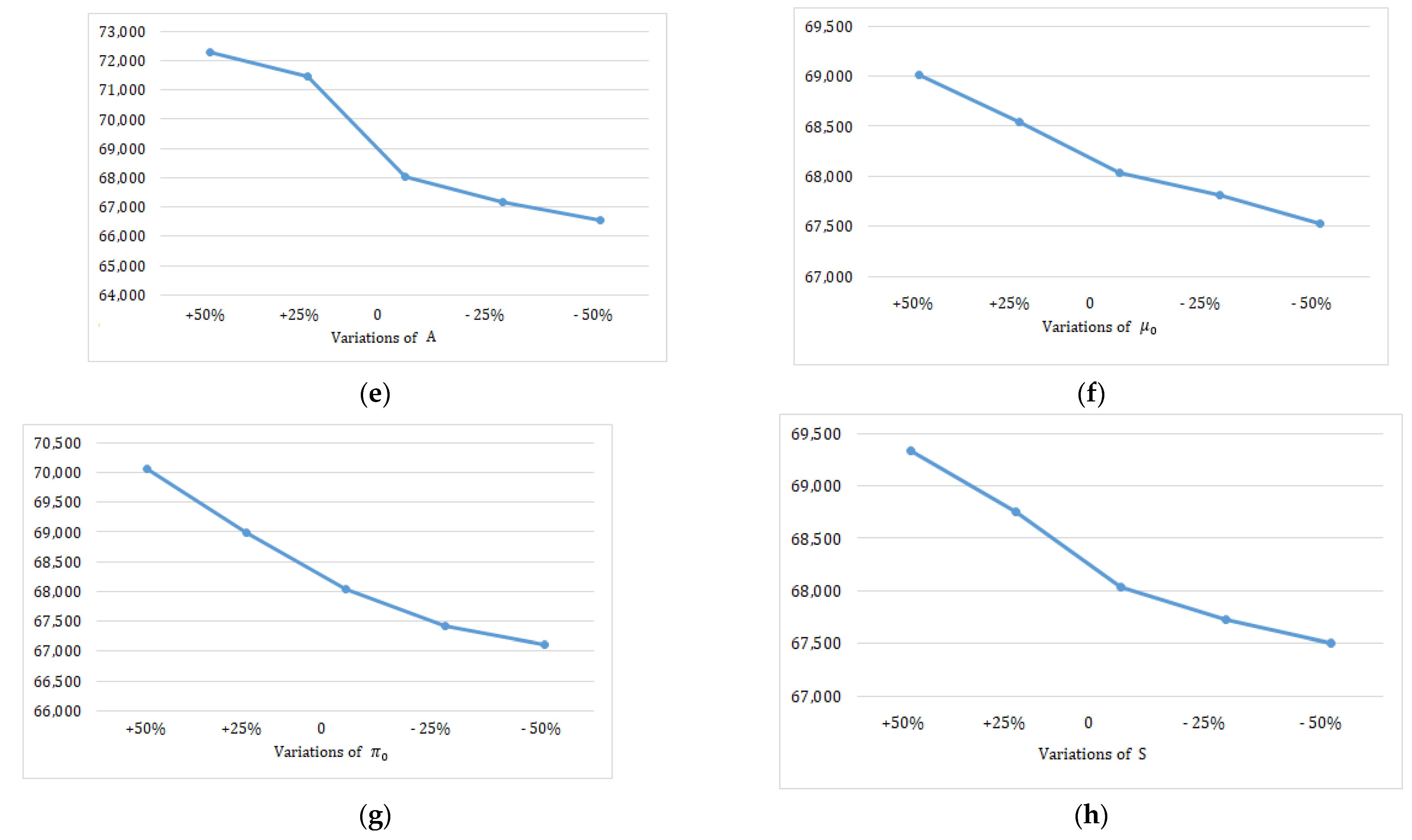
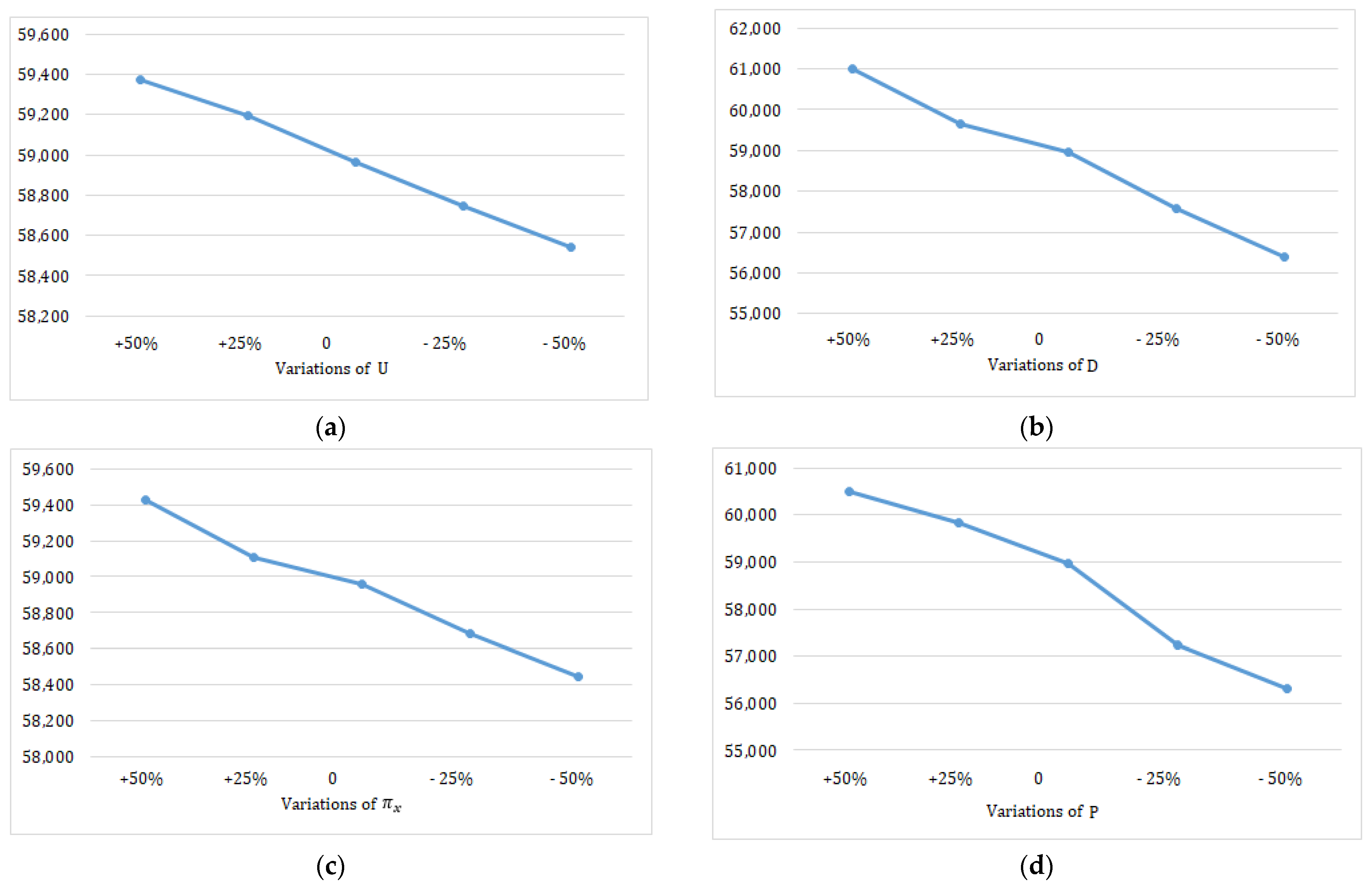
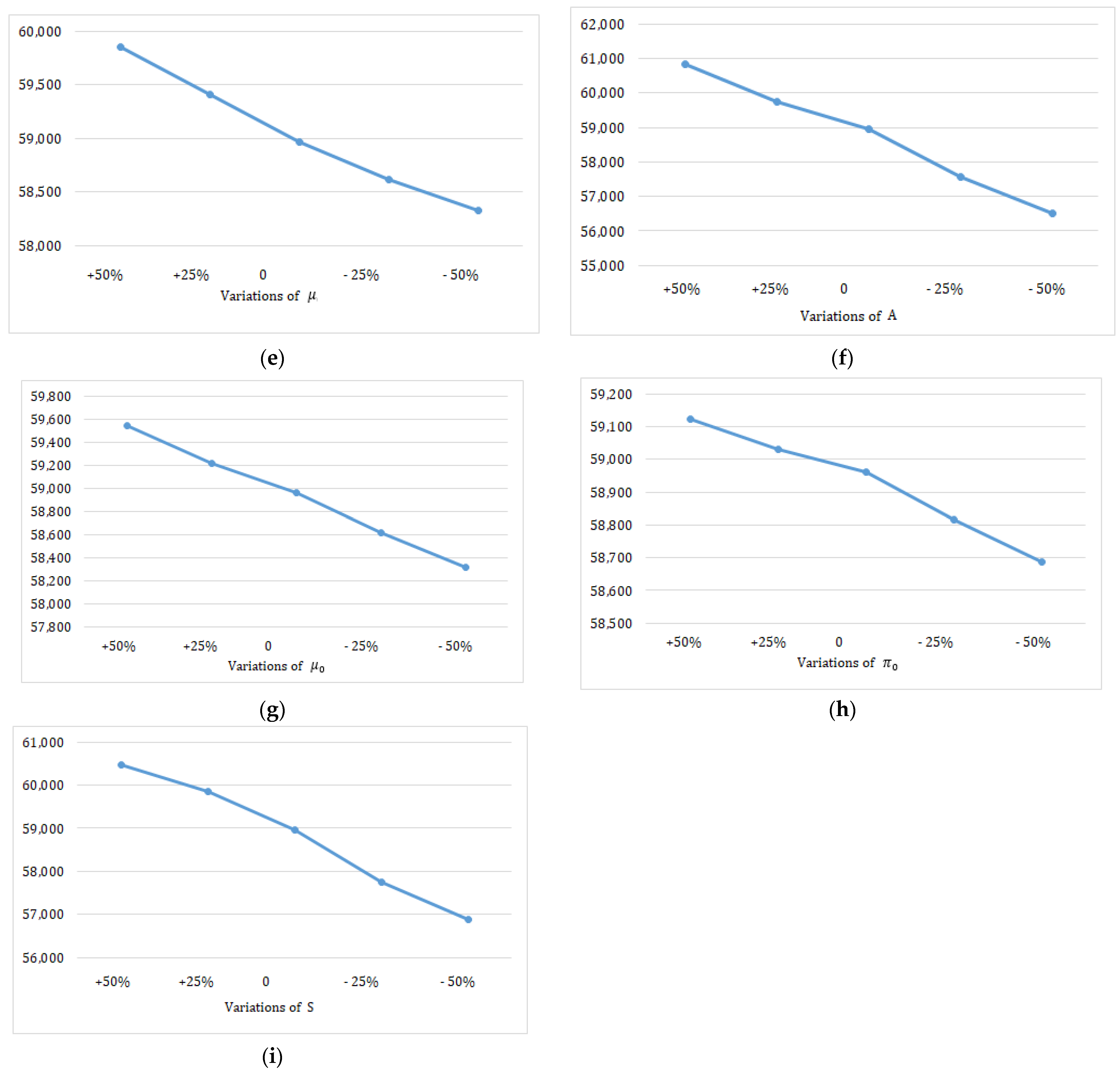
4.2. Sensitivity Study

In this subsection, the sensitivity study is implemented. The findings are provided in

Table 7. Sensitivity analysis (Case I).

Parameters	% Changes	Q*	L*	n*	$\mathit{J}\mathit{E}\mathit{T}{\mathit{C}}_{\mathit{t}}(.)$	Parameters	% Changes	Q*	L*	n*	$\mathit{J}\mathit{E}\mathit{T}{\mathit{C}}_{\mathit{t}}(.)$
D	+50%	2189	4	4	70,701	${\pi }_x$	+50%	2193	4	3	69,874
	+25%	2126	3	3	69,784		+25%	2115	3	3	69,312
	0%	1908	3	3	68,038		0%	1908	3	3	68,038
	−25%	2012	3	3	67,753		−25%	1986	3	3	67,211
	−50%	1986	3	3	65,857		−50%	1915	3	3	67,043
P	+50%	2116	8	4	71,575	$\mu$	+50%	2265	4	4	68,587
	+25%	2095	8	4	69,519		+25%	2187	4	4	68,346
	0%	1908	3	3	68,038		0%	1908	4	3	68,038
	−25%	2011	3	3	67,954		−25%	2016	4	3	67,854
	−50%	1954	3	2	67,123		−50%	1995	4	3	67,532
A	+50%	2214	4	3	72,294	${\mu }_0$	+50%	2206	3	4	69,018
	+25%	2158	4	3	71,456		+25%	2152	3	4	68,542
	0%	1908	3	3	68,038		0%	1908	3	3	68,038
	−25%	2002	3	3	67,157		−25%	1989	3	3	67,816
	−50%	1973	3	2	66,548		−50%	1931	3	3	67,524
${\pi }_0$	+50%	2190	8	3	70,051	S	+50%	2243	4	2	69,339
	+25%	2137	8	3	68,986		+25%	2194	4	2	68,756
	0%	1908	3	3	68,038		0%	1908	3	3	68,038
	−25%	2012	3	3	67,423		−25%	2009	3	3	67,727
	−50%	1969	3	2	67,108		−50%	1899	3	4	67,501

* Optimal values.

and

Table 8. Sensitivity analysis (case II).

Parameters	% Changes	Q	$\mathit{\theta }$	L	n	$\mathit{J}\mathit{E}\mathit{T}{\mathit{C}}_{\mathit{u}}(.)$	Parameters	% Changes	Q	$\mathit{\theta }$	L	n	$\mathit{J}\mathit{E}\mathit{T}{\mathit{C}}_{\mathit{u}}(.)$
D	+50%	6153	0.3	3	2	60,992	${\pi }_x$	+50%	6127	0.3	6	4	59,424
	+25%	6089	0.3	3	2	59,644		+25%	6045	0.3	6	3	59,110
	0%	5987	0.3	3	3	58,962		0%	5987	0.3	3	3	58,962
	−25%	5478	0.3	3	3	57,571		−25%	5876	0.3	3	2	58,681
	−50%	5122	0.4	6	4	56,401		−50%	5743	0.3	3	1	58,448
P	+50%	6248	0.2	8	3	60,491	$\mu$	+50%	6143	0.3	4	3	59,853
	+25%	6107	0.2	8	3	59,847		+25%	6084	0.3	4	3	59,412
	0%	5987	0.3	3	3	58,962		0%	5987	0.3	3	3	58,962
	−25%	5627	0.3	3	2	57,246		−25%	5813	0.3	3	3	58,611
	−50%	5431	0.3	3	2	56,312		−50%	5897	0.3	3	3	58,323
A	+50%	6230	0.3	3	3	60,821	${\mu }_0$	+50%	6150	0.4	6	3	59,540
	+25%	6152	0.3	3	3	59,731		+25%	6091	0.4	6	3	59,215
	0%	5987	0.3	3	3	58,962		0%	5987	0.3	3	3	58,962
	−25%	5148	0.3	3	3	57,576		−25%	5873	0.3	3	2	58,613
	−50%	5019	0.3	3	3	56,521		−50%	5987	0.3	3	2	58,318
${\pi }_0$	+50%	6211	0.4	6	4	59,123	S	+50%	6230	0.3	3	3	60,481
	+25%	6068	0.3	6	3	59,031		+25%	6121	0.3	3	3	59,843
	0%	5987	0.3	3	3	58,962		0%	5987	0.3	3	3	58,962
	−25%	5903	0.3	3	3	58,815		−25%	5843	0.3	3	3	57,760
	−50%	5894	0.3	3	2	58,687		−50%	5725	0.3	3	2	56,877
U	+50%	6254	0.3	3	3	59,374
	+25%	6009	0.3	3	3	59,195
	0%	5987	0.3	3	3	58,962
	−25%	5502	0.3	3	3	58,749
	−50%	5491	0.3	3	3	58,539

as well as in plots, which are shown in Figure 4 and Figure 5.

4.3. Academic and Managerial Implications

Based on the above numerical experiments and results analysis, we propose the following academic and managerial implications:

(1)

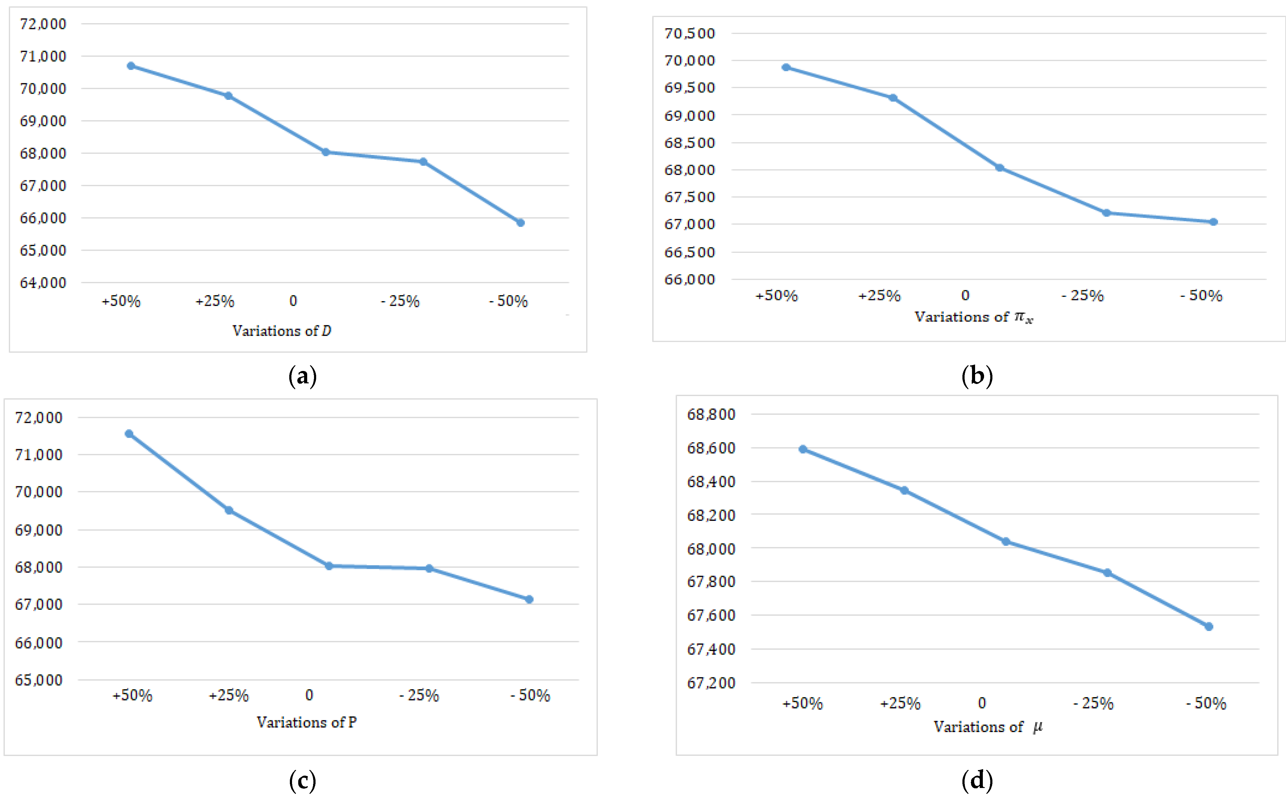
The increase in the backlogged parameters ${\pi }_x$ and ${\pi }_0$ brings a loss in profit, which is a higher total cost as the selling price of the items becomes higher.

(2)

Total cost increases with the increase in $\mu$ and because increasing these values enhances the carbon emissions, and the transportation costs also increase.

(3)

It can be observed from Table 6 and Table 7 that when 𝐴 decreases, the joint expected total cost also decreases. This result is not unexpected, because in practice when the buyer controls their ordering cost, the total inventory cost automatically decreases.

(4)

Table 7 and Table 8 indicate that with the increase in the parameters $(D,P,A,{\pi }_0{\pi }_x,$ $\mu ,{\mu }_0,S)$ there is an increase in $JET{C}_t(.)$,$JET{C}_u(.)$, and $Q$. $L$ is moderately sensitive, while n is less sensitive. Managers should understand the misclassification errors’ effect on decision-making, as shown in the results of the model.

(5)

The costs incurred by the vendor increase due to the increase in S, which leads to an increased joint total cost. The vendor’s setup cost is also highly sensitive to Q and n.

(6)

As the customer demands increase, the vendor will plan a larger number of shipments, thus resulting in higher emissions. One solution to curtail emissions is to reduce delivery frequency, which will result in a longer lead time.

(7)

Table 8 indicates that with an increase in the vendor’s limited carbon emission quantity $\left(U\right)$, an increase in $JET{C}_u(.)$ is also recorded. The high limited carbon emissions allowed by governments may lead to the vendor producing more products. Nonetheless, increasing carbon emissions $\left(U\right)$ limits are not always a positive option for reducing carbon emissions. Defining appropriate carbon emission strategies that align economic development with ecological protection is important for governments.

(8)

The suggested technique lets managers change the rate of production by managing production allocation. When the rate of production has a significant influence on the quantity of the emissions that are produced, the plan of a $P$ adjustment becomes vital. Our findings show that adjusting the $P$ to a suitable level can benefit the system by balancing the supply with the demand and cutting emissions. Regrettably, prior inventory models did not take such restrictions into account; hence, this benefit was unavailable.

(9)

This study evaluates the consequences of carbon control depending on emissions, the goal function of the suggested inventory system, and inventory cost. The cost of the system among different scenarios (carbon taxation and limited carbon emission) are compared. The results indicate that limited carbon emission is less than carbon taxation for the inventory cost system.

(10)

The comparison between carbon taxation and limited carbon policies reveals that subsequent costs to the buyer exert varying effects on the vendors’ total costs and carbon emissions.

(11)

With the help of green technology, the vendor has more chances to cut the emissions caused by the production activity. Although the use of green technology needs a greater cost, the vendor will obtain the benefits from the reduced emissions.

(12)

Purchasing power allowances can be reduced by investment in decreasing carbon outflows, even for a lesser limit for carbon emissions.

(13)

Managers can only invest in renewable methods that lead to a reduction in carbon discharges and meet the requirements for lower pollution levels, which leads to a maximum aggregate inventory cost. The total cost for inventory then decreases as the carbon-release cap slowly rises. The aggregate inventory cost is retained at a given cost when the carbon emission limit rises above a threshold, which makes the SC limited by the carbon emission limit.

(14)

According to our findings, transitioning to green production has a significant influence on the inventory system. In order to comply with carbon tax legislation, the producer can use green technology to reduce emissions from the activities of production, transportation, and storage. Unfortunately, with various types of green technology available, picking which one to employ in production may be challenging. Green technology includes renewable energy, green chemistry, and recycling technology (100% recycled tin, precious metals). Consequently, administrators must cautiously select the most appropriate green technology. In addition to cost reasons, managers must evaluate other variables when selecting the appropriate technology.

(15)

The proposed model gives flexibility to a manager to adjust the production rate by controlling the production allocation. In a situation where the level of production emissions is very much influenced by the production rate, the policy on production-rate adjustment becomes important. Our study shows that by adjusting the production rate to an appropriate level, the system can obtain benefits, balancing the production with demand and decreasing the production’s emissions.

5. Conclusions

There is growing pressure in many nations to reduce carbon emissions with few objectives, to reduce emissions or the minimal preparations being affected to lower emissions to prevent climatic change. Moreover, the expectations at the quality level set by the consumer should be met by the production system because of the impact of human error on issues such as productivity, customer service quality, and decision-making. Therefore, all industrial sectors need to undertake efforts to evade human error and minimize emissions. The impact of human errors and renewable methods on a complex SC system, by considering carbon emissions during product production transportation and storage, was addressed here. Limited total carbon emissions and carbon taxes were the carbon emission strategies considered in this study. To minimize the system cost in various carbon emission strategies, the model could be applied to any complex system to obtain a sensitive solution for the developed operating optimum conditions and the amounts to spend on green investment. This study has also outlined the need for governments to adopt relevant policies to protect the environment. An expert system for optimum decision-making could be obtained for the best decision-making solution.

This research could be expanded to include many goods in the future. This may be conducted by contemplating customers who purchase items from different sellers. In addition, the inventory model’s service-level restrictions and periodic review procedures can be used to expand the current research. The model may be expanded to include numerous objective optimizations based on the production system’s desire for sustainability. Another major concern with this study’s proposed condition is the unclear condition, which can be addressed in future studies.

References

1. Arora, V.; Chan, F.T.; Tiwari, M.K. An integrated approach for logistic and vendor managed inventory in supply chain. Exp. Syst. App. 2010, 37, 39–44. [Google Scholar] [CrossRef]
2. Tempelmeier, H.; Bantel, O. Integrated optimization of safety stock and transportation capacity. Euro. J. Operat. Res. 2015, 247, 101–112. [Google Scholar] [CrossRef] [Green Version]
3. Khanra, S.; Ghosh, S.K.; Pathak, C. A three-layer supply chain integrated production-inventory model with idle cost and batch shipment policy. Sust. Anal. Model. 2022, 2, 100011. [Google Scholar] [CrossRef]
4. Das, B.C.; Das, B.; Mondal, S.K. An integrated production-inventory model with defective item dependent stochastic credit period. Comp. Indust. Eng. 2017, 110, 255–263. [Google Scholar] [CrossRef]
5. Nezamoddini, N.; Gholami, A.; Aqlan, F. A risk-based optimization framework for integrated supply chains using genetic algorithm and artificial neural networks. Int. J. Prod. Econ. 2019, 225, 107569. [Google Scholar] [CrossRef]
6. Priyan, S.; Mala, P. Optimal inventory system for pharmaceutical products incorporating quality degradation with expiration date: A game theory approach. Oper. Res. Health Care 2020, 24, 100245. [Google Scholar] [CrossRef]
7. Khan, M.; Jaber, M.Y.; Bonney, M. An economic order quantity (EOQ) for items with imperfect quality and inspection errors. Int. J. Prod. Econ. 2011, 133, 113–118. [Google Scholar] [CrossRef]
8. Priyan, S.; Uthayakumar, R. Mathematical modeling and computational algorithm to solve multi-echelon multi-constraint inventory problem with errors in quality inspection. J. Math. Model. Algo. Oper. Res. 2015, 14, 67–89. [Google Scholar] [CrossRef]
9. Zhou, Y.; Chen, C.; Li, C.; Zhong, Y. A synergic economic order quantity model with trade credit, shortages, imperfect quality and inspection errors. App. Math. Model. 2016, 40, 1012–1028. [Google Scholar] [CrossRef]
10. Khan, M.; Ahmad, A.R.; Hussain, M. Integrated decision models for a vendor–buyer supply chain with inspection errors and purchase and repair options. Int. J. Adv. Manuf. Tech. 2019, 104, 3221–3228. [Google Scholar] [CrossRef]
11. Taheri-Tolgari, J.; Mohammadi, M.; Naderi, B.; Arshadi-Khamseh, A.; Mirzazadeh, A. An inventory model with imperfect item, inspection errors, preventive maintenance and partial backlogging in uncertainty environment. J. Indust. Manag. Opt. 2019, 15, 1317. [Google Scholar] [CrossRef]
12. Tiwari, S.; Kazemi, N.; Modak, N.M.; Cárdenas-Barrón, L.E.; Sarkar, S. The effect of human errors on an integrated stochastic supply chain model with setup cost reduction and backorder price discount. Int. J. Prod. Econ. 2020, 226, 107643. [Google Scholar] [CrossRef]
13. Feng, L.; Tao, J.; Richard, Y.K.F.; Peng, W. Impacts of inspection rate on integrated inventory models with defective items considering capacity utilization: Rework-versus delivery-priority. Comput. Ind. Eng. 2021, 156, 107245. [Google Scholar]
14. Wakhid, A.J. Sustainable inventory management for a closed-loop supply chain with energy usage, imperfect production, and green investment. Clean. Logist. Supply Chain. 2022, 4, 100055. [Google Scholar]
15. Subhajit, D.; Rajan, M.; Ali, A.S.; Asoke, K.B. An application of control theory for imperfect production problem with carbon emission investment policy in interval environment. J. Frankl. Inst. 2022, 359, 925–1970. [Google Scholar]
16. Liao, C.J.; Shyu, C.H. An analytical determination of lead time with normal demand. Int. J. Oper. Prod. Manag. 1991, 11, 72–78. [Google Scholar] [CrossRef]
17. Pan, J.C.H.; Yang, J.S. A study of an integrated inventory with controllable lead time. Int. J. Prod. Res. 2002, 40, 1263–1273. [Google Scholar] [CrossRef]
18. Hoque, M.A. An alternative model for integrated vendor–buyer inventory under controllable lead time and its heuristic solution. Int. J. Syst. Sci. 2007, 38, 501–509. [Google Scholar] [CrossRef]
19. Modak, N.M.; Kelle, P. Managing a dual-channel supply chain under price and delivery-time dependent stochastic demand. Europ. J. Operat. Res. 2019, 272, 147–161. [Google Scholar] [CrossRef]
20. Benjaafar, S.; Li, Y.; Daskin, M. Carbon footprint and the management of supply chains: Insights from simple models. IEEE Trans. Autom. Sci. Eng. 2012, 10, 99–116. [Google Scholar] [CrossRef]
21. Hammami, R.; Nouira, I.; Frein, Y. Carbon emissions in a multi-echelon production-inventory model with lead time constraints. Int. J. Prod. Econ. 2015, 164, 292–307. [Google Scholar] [CrossRef]
22. Li, J.; Su, Q.; Ma, L. Production and transportation outsourcing decisions in the supply chain under single and multiple carbon policies. J. Clean. Prod. 2017, 141, 1109–1122. [Google Scholar] [CrossRef]
23. Tang, S.; Wang, W.; Cho, S.; Yan, H. Reducing emissions in transportation and inventory management: (R, Q) policy with considerations of carbon reduction. Europ. J. Operat. Res. 2018, 269, 327–340. [Google Scholar] [CrossRef]
24. Halat, K.; Hafezalkotob, A. Modeling carbon regulation policies in inventory decisions of a multi-stage green supply chain: A game theory approach. Comp. Indust. Eng. 2019, 128, 807–830. [Google Scholar] [CrossRef]
25. Huang, Y.S.; Fang, C.C.; Lin, Y.A. Inventory management in supply chains with consideration of logistics, green investment and different carbon emissions policies. Comp. Indust. Eng. 2020, 139, 106207. [Google Scholar] [CrossRef]
26. Tiwari, S.; Ahmed, W.; Sarkar, B. Sustainable ordering policies for non-instantaneous deteriorating items under carbon emission and multi-trade-credit-policies. J. Clean. Prod. 2019, 240, 118183. [Google Scholar] [CrossRef]
27. Yadegaridehkordi, E.; Hourmand, M.; Nilashi, M.; Alsolami, E.; Samad, S.; Mahmoud, M.; Alarood, A.A.; Zainol, A.; Majeed, H.D.; Shuib, L. Assessment of sustainability indicators for green building manufacturing using fuzzy multi-criteria decision-making approach. J. Clean. Prod. 2020, 277, 122905. [Google Scholar] [CrossRef]
28. Yang, W.; Pan, Y.; Ma, J.; Yang, T.; Ke, X. Effects of allowance allocation rules on green technology investment and product pricing under the cap-and-trade mechanism. Energy Pol. 2020, 139, 111333. [Google Scholar] [CrossRef]
29. Md. Rakibul, H. Optimizing inventory level and technology investment under a carbon tax, cap-and-trade and strict carbon limit regulations. Sust. Prod. Cons. 2021, 25, 604–621. [Google Scholar]
30. Sarkar, B.; Kar, S.; Basu, K.; Guchhait, R. A sustainable managerial decision-making problem for a substitutable product in a dual-channel under carbon tax policy. Comp. Indus. Eng. 2022, 172, 108635. [Google Scholar] [CrossRef]
31. Yuqiang, F.; Yankui, L.; Yanju, C. A robust multi-supplier multi-period inventory model with uncertain market demand and carbon emission constraint. Comput. Ind. Eng. 2022, 165, 107937. [Google Scholar]
32. Kavina, K. 2019. Available online: https://www.nrx.com/human-error-in-manufacturing/#:~:text=One%%2020definition%20is%%2020%%20E2%80%9Ca%20person%E2%80%99s,there%20was%20no%20harm%20intended (accessed on 12 October 2022).
33. Doe Standard. Human Performance Improvement Handbook: Human Performance Tools for Individuals, Work Teams, and Management; U.S. Department of Energy: Washington, DC, USA, 2009; Volume 2. [Google Scholar]
34. Simione. 2008. Available online: https://www.climateaction.org/news/scrap_metal_recycling_plays_crucial_role_in_climate_change (accessed on 12 October 2022).
Figure 1. Vendor–buyer inventory structure.
Sustainability 14 16082 g001
Figure 2. Graphical picture of results for Case I.
Sustainability 14 16082 g002
Figure 3. Graphical picture of results for Case II.
Sustainability 14 16082 g003
Figure 4. Plots of the sensitivity analysis (Case I). (a) Effects of D on J E T C t ( . ) ; (b) effects of π x on J E T C t ( . ) ; (c) effects of P on J E T C t ( . ) ; (d) effects of μ on J E T C t ( . ) ; (e) effects of A on J E T C t ( . ) ; (f) effects of μ 0 on J E T C t ( . ) ; (g) effects of π 0 on J E T C t ( . ) ; (h) effects of S on J E T C t ( . ) .
Sustainability 14 16082 g004aSustainability 14 16082 g004b
Figure 5. Plots of the sensitivity analysis (Case II). (a) Effects of U on J E T C u ( . ) ; (b) effects of D on J E T C u ( . ) ; (c) effects of π x on J E T C u ( . ) ; (d) effects of P on J E T C u ( . ) ; (e) effects of μ on J E T C u ( . ) ; (f) effects of A on J E T C u ( . ) ; (g) effects of μ 0 on J E T C u ( . ) ; (h) effects of π 0 on J E T C u ( . ) ; (i) effects of S on J E T C u ( . ) .
Sustainability 14 16082 g005aSustainability 14 16082 g005b