Do Rainfall Shocks Prompt Commercial Input Purchases Amongst Smallholder Farmers in Diverse Regions and Environments in Malawi?

Abstract

The ability of farmers to acquire inputs through purchase from available markets empowers them with the autonomy and capacity to diversify inputs, consequently enhancing the resilience of their cropping activities to various shocks. This paper investigates whether climate shocks, particularly rainfall shocks, influence commercial input purchase decisions by smallholder farmers in contrasting geographic regions in Malawi, with a particular emphasis on fertilizer, agrochemicals, seed, and labor. The empirical approach integrates historical weather information, climate shock perceptions with a longitudinal household survey data set to model commercial input purchasing decisions using appropriate latent variable models. The findings suggest that exposure to recent rainfall shocks, especially droughts, stimulates commercial input purchasing across regions, especially in drier central and southern regions of Malawi. This result holds true for general input purchase decisions and for specific inputs such as agrochemicals, fertilizer, seed, and labor. Although drought shocks considerably increase the probability of acquiring inputs through purchase, they occasionally diminish the intensity of purchases. Both objective and subjective measures of lagged rainfall shocks are revealed as significant determinants of commercial input purchases across regions in Malawi. In addition to regional heterogeneity findings, further analysis shows that the relatively wealthier, male-headed families and those with access to information are more likely to invest in purchased inputs in response to drought shocks. Scaling up policies that remove demand- and supply-side barriers to smallholder farmers’ access to commercial inputs from available markets is necessary for adaptation to rainfall shocks.

1. Introduction

Agriculture in Sub-Sahara Africa (SSA) is primarily rain-fed, causing it to be highly vulnerable to climate change, especially weather shocks. An estimated 95% of farmland across SSA is rain-fed, of which over 80% of all the farmland is managed by smallholder farmers, causing smallholder farming to be highly sensitive to extreme weather events such as drought and floods [1]. Weather shocks such as drought and floods significantly reduce crop production and yields and, in extreme cases, risk total crop failure with severe implications on incomes and food security [2,3,4]. The direct implication is that failure by smallholder farming systems to adapt to the changing climate can significantly hurt agro-based economies’ current and future social and economic prospects. This idea is particularly true in Malawi, where exposure to extreme weather events such as drought and floods has led to significant crop losses, occasional displacement of people, loss of life, infrastructure damage, poverty traps, and obstruction of development [4,5,6].

Building the resilience of smallholder agriculture to weather shocks is paramount to curb the negative impacts of climate shocks. One way to improve farming systems’ resilience is by altering agricultural input use. Failure by smallholder farmers to adapt to the changing climate through altering agricultural input use and farming practices could worsen agricultural outcomes. However, investing in modern input use and production technologies that allow for and promote diversity is found to provide a better strategy for strengthening agricultural production in the face of increased production risk from climate change [7,8,9]. In the context of SSA and particularly in a country such as Malawi with weak and/or inefficient formal markets for labor, inputs/outputs, insurance, and credit, adopting a portfolio of inputs and farming strategies that offer protection against weather risk is important for smallholder farmers [10,11,12]. Access to purchased inputs can offer the farmer the potential to adapt to the changing climate. This is because, ceteris paribus, input purchasing offers the smallholder farmer autonomy to change the input mix in ways that improve the resilience of their cropping activities to climate change. Through input purchases, farmers can: (i) diversify crops and/or crops varieties (improved, local, drought-tolerant varieties), (ii) diversify fertilizer use through organic and inorganic fertilizer purchases, (iii) diversify crop and crop harvest protection methods by complementing natural methods with agrochemical use, and (iv) respond to labor shortages through hiring off-farm labor. Given that smallholder farmers historically are known to rely on traditional farming inputs such as organic fertilizers (manure, compost), local (traditional) seed varieties, natural crop protection methods, and the use of family labor, input purchases are highly important as a conduit of adding new and/or modern inputs to the farming input portfolio. Hence, access for smallholder farmers to purchased inputs is vital for building small-scale farming systems that are resilient to climate change.

However, the use of modern inputs and other climate-resilient technologies in SSA is low compared to other regions, although recent evidence shows a steady increase over time [13]. Various reasons have been explored in the literature to explain the low use rates for modern inputs and technologies in SSA. For instance, the low use of modern fertilizers is attributed to: (i) lack of capital to purchase fertilizers [14,15], (ii) low profitability of fertilizers on highly degraded African soils, (iii) lack of agricultural insurance causing it to be too risky to invest in fertilizers [16], and (iv) input and output market inefficiencies causing high fertilizer investments to be less profitable. Besides, studies have also shown that high seed prices, unavailability of seeds in local markets, lack of adequate access to information, and unavailability of some seed attributes in improved varieties are key reasons for the low use of modern varieties [15,17,18]. Similar factors are acknowledged in the literature as key impediments to the adoption of modern technologies in agriculture, including climate-resilient inputs [19,20].

This work argues that climate variables, temperature and rainfall, variability in climate factors, and persistent exposure to climate shocks (flood or drought) alter the need for adopting high-input agriculture. This view makes a plausible assumption given that theories of farmer behavior under risk (e.g., the state-contingent theory by Chambers and Quiggin [21]) reveal weather expectations and past climate shock exposures to be key determinants of farming behavior. In addition, given the overwhelming evidence that climate risk factors significantly reduce crop yield in developing regions (see Kurukulasuriya and Rosenthal [22] for a review), it is also highly probable that climate risk factors alter input demand [23]. Thus, understanding the effects of climate risk on commercial input purchasing is important for adaptation policy. Our specific objectives in this paper are as follows:

(a)

To determine how long-term climate and lags in rainfall shocks affect the sourcing of off-farm agricultural inputs (fertilizer, agrochemicals, seed, and labor) through purchase by smallholder farmers in Malawi.

(b)

To examine the role of regional and socioeconomic heterogeneity in shaping the impacts of climate risk on the sourcing and use of commercially purchased inputs.

We build on previous studies that evaluate the influence of climate risk on the choice and use of agricultural inputs and climate-resilient technologies such as modern agricultural inputs (e.g., Mendelsohn and Wang [23]), the use of drought-tolerant maize technologies (e.g., Holden and Quiggin [24] and Katengeza, Holden, and Lunduka [11]), the use of integrated soil fertility management (ISFM) technologies (e.g., Katengeza et al. [25]), and the sources or types of purchased seeds (e.g., Nordhagen and Pascual [12]) and evaluate the influence of climate risk factors in shaping the use of commercially purchased inputs in heterogeneous settings in Malawi. Our study adds to this literature by generating evidence specifically on the influence of climate risk in shaping commercial input purchasing for key inputs (fertilizers, agrochemicals, seeds, and labor) in Malawi. We further improve on the previous related literature by focusing on the potential influence of spatial heterogeneity (regional differences), socioeconomic inequality, and access to agriculture information in shaping commercial input purchasing responses to climate risk factors. We also test the impact of rainfall shocks using both (i) objective measures of rainfall shocks and (ii) subjective measures of rainfall shocks (i.e., farmer perceptions data on shock exposure in the recent past). Most importantly, we derive implications for climate change adaptation through market development in Malawi. We rely on multiple rounds of the novel, longitudinal nationally representative Livelihood Standards Measurement Survey-Integrated Surveys on Agriculture (LSMS–ISA) datasets collected from smallholder farming households in Malawi in 2011, 2015, and 2019, combined with historical monthly weather data. Our empirical approach adopts suitable latent variable approaches [26] to analyze the influence of climate risk on commercial input purchasing in Malawi’s smallholder farming.

The rest of this paper is organized as follows. Section 2 briefly documents the impacts of climate change on agricultural development in Malawi, while Section 3 outlines the study’s theoretical framework. Then, Section 4 presents the study’s methodology and Section 5 and Section 6 present the main findings and discussions, respectively. Lastly, Section 7 concludes the paper and provides policy implications.

2. Climate Change and Agriculture Development in Malawi: A Snapshot

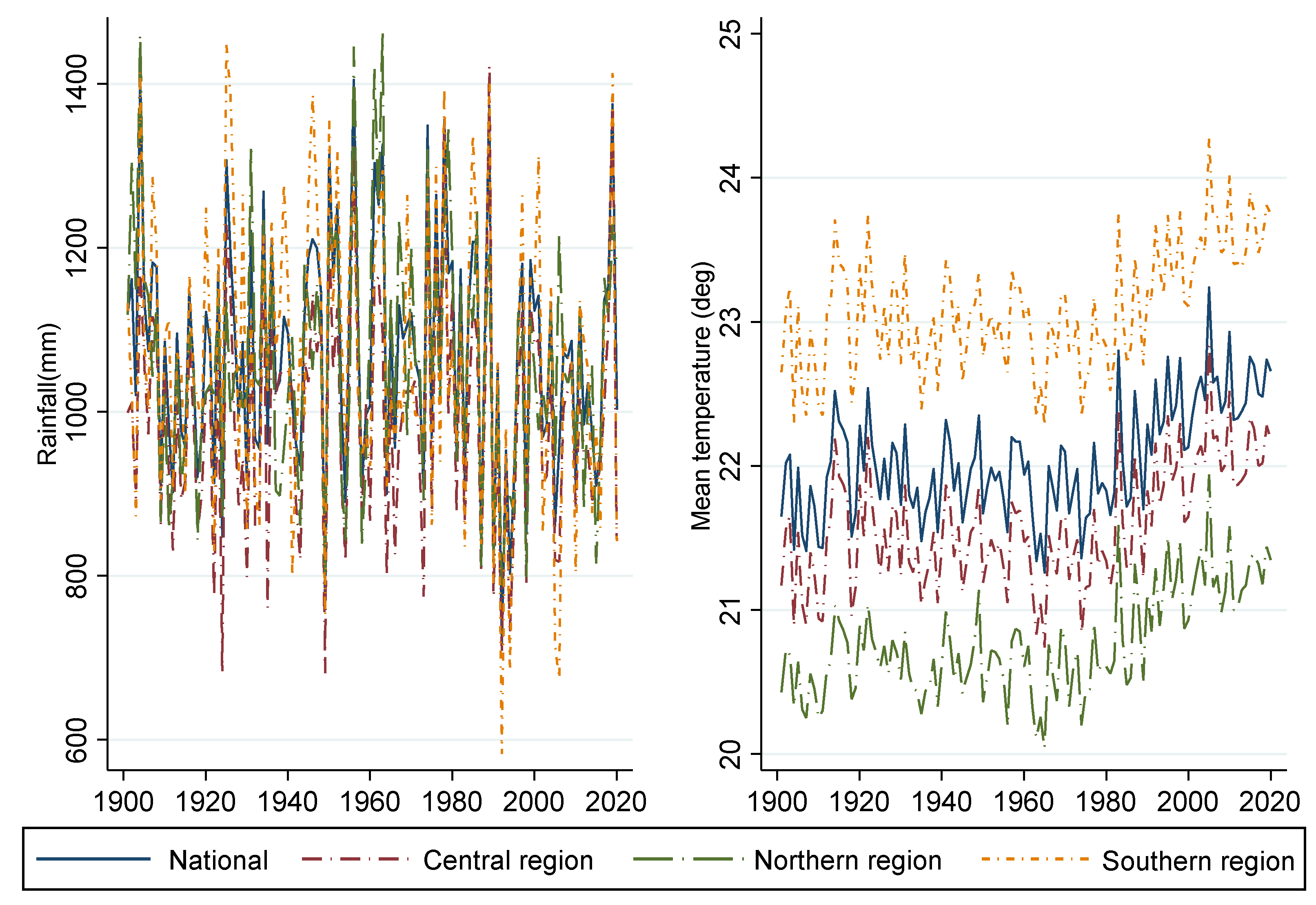
Malawi is characterized by two distinct seasons: the rainy season, which runs from November to April, and the dry season, which runs from May to October. The rainy season is the dominant season for crop production. Temperature and rainfall are variable with seasons and topography. The lowest average temperatures are experienced in the dry season, specifically in the month of July (from 12–15 °C) in the highland areas (northern region), while the warmest temperatures (25–26 °C) are experienced in the lowlands (southern region) during the rainy season usually in October. Annual rainfall ranges from as low as 500 mm in the lowlands to more than 1500 mm in the highlands. Rainfall is highly variable and its variability is highly linked to the El Niño Southern Oscillations (ENSO) or El Niño/La Niña teleconnections [6,27,28]. The El Niño and La Niña teleconnections are strongly linked to probable drought and flood events, respectively [6]. We summarize historical climate variables (temperature and rainfall) for Malawi (national) and for the main geographical regions (northern, central, and southern regions) based on observed historical data produced by the Climatic Research Unit (CRU) of the University of East Anglia in Figure 1. Figure 1 shows the historical average annual rainfall trends for Malawi from 1901–2019. Rainfall variability over the years is evident, with an increasing rainfall trend from 1901 to 1960 and a decreasing trend afterward. The average mean temperature shows an increasing trend from 1901 to the present, with the southern regions having the highest average temperatures compared to the northern region (lowest) and central regions (in the middle) (Figure 1).

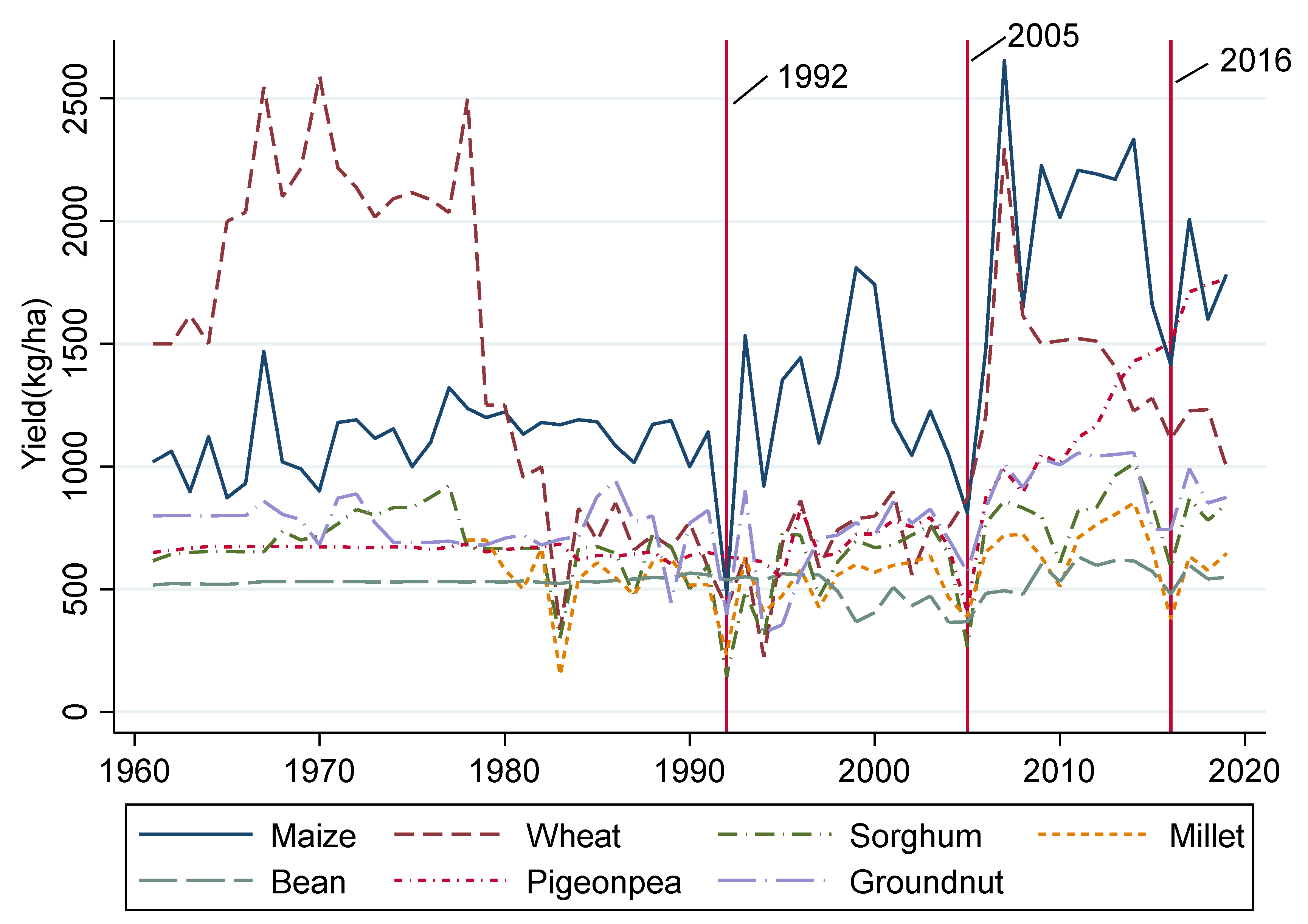
Several unique characteristics make Malawi highly vulnerable to climate variability and change. Some of these include high dependence on rain-fed agriculture and Maize as a staple crop, high population growth, high poverty rates, malnutrition, and disease pandemics (e.g., HIV/AIDS) [28,29,30]. Extreme climate events such as drought, floods, and elevated temperatures negatively impact agricultural production, water resources, fisheries, ecosystems, and human health [6,28]. Of importance to this study are the direct effects of extreme weather events on agricultural production. Extreme weather events such as droughts and floods and significant seasonality changes negatively affect Malawi’s agricultural production. Drought and flood events have increased in frequency and intensity in the past two to three decades. For example, agricultural production (for Maize and other food crops) has been significantly low in drought years such as in 1991/92, 2001/02, 2004/5, and 2015/16 [5,6,31]. In Figure 2, we plot the agricultural productivity trends for selected main food crops in Malawi and demonstrate an association between a fall in yields and the occurrence of selected drought events in the recent past (1991/92, 2004/5, and 2015/16). The most recent drought event experienced in 2015/16 was characterized by a delayed onset of the agricultural season, leading to severe crop failure mostly in the central and southern regions [32].

The overall implication is that climate change is a reality in Malawi and it has had several negative impacts on agricultural production, water resources, ecosystems, food security, and on the Malawian citizenry’s overall well-being, particularly the rural population. The consequences of climate change on rural livelihoods are dire because agriculture remains one of the country’s most important economic activities. For instance, the agricultural sector contributes nearly 33% of the Gross Domestic Production (GDP) and nearly 80% of the employment [33]. Therefore, it is important to understand how climate risk influences smallholder farmers’ decisions to invest in commercially purchased inputs as a potential adaptation mechanism in contrasting regions and other socioeconomic settings in Malawi.

3. Theoretical Framework: Use of Purchased Inputs under Increased Climate Erraticism

3.1. Why Invest in Commercial Input Purchases with Increasing Climate Erraticism

Farmers in Malawi can source agricultural inputs from both informal and formal channels. Formal input sources in Malawi include public and private agricultural markets (e.g., the Agricultural Development and Marketing Corporation (ADMARC), other private or public markets), and government support programs (e.g., Farm Input Subsidy Program (FISP)). Informal input sources mainly include farmers’ social networks and other sources not supervised by any organization. In both formal and informal sources of agricultural inputs, farmers access inputs through some form of trade (e.g., purchasing) or barter. Access to inputs in the formal market is mainly through cash (or credit) purchases, while from informal sources, purchases are in cash, barter, or kind. Having access to purchased inputs is highly important in the context of elevated climate risk. It offers the farmer the autonomy and ability to change their input mix to improve the resilience of their agricultural activities. Although government programs such as FISP have become an important supplementary source of agricultural inputs, available evidence reports that such programs target a selection of farmers based on their underlying objectives [34]. In addition, some of the agricultural support programs, such as FIPS in Malawi, are reported to have been marked with irregularities in voucher distribution [34,35]. Hence, not all farmers in need have access to them. Besides, farmers with access to FISP may not access all inputs of their choice and their demand, leaving other sources of inputs, such as commercial input purchasing, equally important to complement inputs from other sources.

Increased climate variability may render conventional farming inputs less favorable, which calls for modern inputs that can enhance resilience. For instance, climate variability and change are associated with increased pests and diseases [36], which may increase the need for agrochemicals. For instance, in some parts of Malawi, rainfall variability in the form of dry spells and floods has been associated, respectively, with increased fall armyworm and Striga infestation in Maize fields [37]. Additionally, using traditional crop varieties with increased climate risk renders crop yields more vulnerable [38], which calls for the diversification of local with improved varieties. For instance, in Malawi, drought-tolerant maize varieties have been proven to enhance the resilience of maize yields to climate stress [39,40]. The implication is that access to purchased seeds may allow farmers to diversify the conventional seed varieties with more resilient varieties available on the market. In addition, input purchasing offers the farmer the chance to access organic and chemical fertilizers, which are beneficial under a changing climate. On-farm organic fertilizer sources may become less reliable with increased climate variability (e.g., through the loss of livestock due to diseases and pests), which demands farmers complement traditional (on-farm) sources with off-farm sources. Besides, access to chemical fertilizer allows the farmer to implement micro-dosing techniques that are proven to offer sufficient nutrition in highly degraded soil in a sustainable fashion [41,42]. Fertilizer purchasing can aid the farmer in supplementing fertilizer requirements to enhance the resilience of farming activities under a changing climate. Likewise, adapting to climate change may require supplementing family labor with off-farm labor. Supplementing family labor can be beneficial when the household faces labor shortages or when new skills are required to implement innovations or technologies effectively. For instance, climate-smart practices such as Conservation Agriculture (CA) may increase labor demand at the household level [43], increasing the need to hire laborers off-farm.

Commercial input purchases are important for two reasons: (a) response to input shortages and (b) as a conduit for adding new or modern inputs to the farming input portfolio. Overall, input purchases increase access to inputs and diversity, enhancing resilience to climate change. Besides, when farmers improve their participation in markets, it also supports the prospects of reviving agricultural markets, which are usually deemed dysfunctional (weak) and not fit for purpose [44], with overall positive implications for broader society. However, it is important to acknowledge that commercial input purchasing, although an essential source of inputs, has some limitations. Input markets in SSA, including Malawi, are imperfect [34,44], and hence access to inputs by farmers is marred with pervasive transaction costs. These high transaction costs and the lack of purchasing power by farmers limit the access to purchased inputs. However, market players’ innovative practices in selling inputs work against these challenges. For example, seed companies have been selling inputs (seed) in varied bag sizes [14,45] and the literature (e.g., Duflo et al. [46] and Holden and Lunduka [47]) confirms that the timing of input supply by input providers influences demand. These are a few examples of innovative approaches by input providers in the developing world that raise prospects for farmers to purchase inputs despite their credit and other access constraints.

3.2. Analyzing the Use of Purchased Inputs under Elevated Climate Risk

Following previous studies that have analyzed the adoption and impact of selected agriculture technologies under production risks (e.g., drought-tolerant maize technologies [11,24,39] and integrated soil fertility management technologies [25] to mention just a few), we can study farmers’ responses to climate risk through commercial input purchasing using the state-contingent theory of Chambers and Quiggin [21]. The state-contingent model assumes $q$ distinct outputs, $v$ distinct inputs, and $n$ possible states of nature. The smallholder farming household allocates input $v\in {\Re }_{+}^V$ and chooses state-contingent output $q\in {\Re }_{+}^{N*Q}$ ex ante (before the state of nature is revealed). ${\Re }_{+}$ implies that $v$ and $q$ are positive real numbers. The output is then produced after the state of nature is revealed (ex post) with inputs fixed. If the smallholder farming household chooses output $q$ and the state of nature $n$ is realized, then the observed output will be $q_n$.

The state of technology ($K$) can be summarized as $K=\left[\left(v,q\right):v \to (\mathrm{can}\mathrm{produce}) q\right]$. If we designate the price of inputs and outputs as $p_v$ and $p_q$, respectively, then we can express the technology ($K$) either as a demand function of the form: $v\left(p_v,q\right)=argmin \left[p_{v}v:\left(v,q\right)\in K\right]$, or as a cost function of the form: $CF\left(p_v,q\right)=min\left[p_{v}v:\left(v,q\right)\in K\right]$. If we assume a simple case of only two states of nature, one of which is unfavorable (vs. a favorable state), the smallholder farmer’s interest will be to maximize output ($q$). The smallholder farmer’s problem is to make a decision under uncertainty where state one (1) is unfavorable only if the output $q_1<q_2$. In such a setting, it is possible to distinguish between inputs that are risk-substituting and those that are risk-complementary [11,21,24]. Input $v_j$ is risk complementary [risk substituting] if a shift from a state-contingent output vector $q$ to a riskier output vector $q^{\prime }$ leads to an increase [decrease] in demand for input $v_j$ that is: $v_j\left(p_v, q\right)\langle v_j\left(p_v,q^{\prime }\right) [v_j\left(p_v, q\right)\rangle v_j\left(p_v,q^{\prime }\right)]$.

The definition of risk-substituting inputs implies that an exogenous increase in risk (e.g., climate risk) will lead to an increase in the share of risk-substituting inputs in the input mix for a given expected output. Therefore, based on this theoretical framework, we hypothesize that exogenous exposure to climate risk (rainfall shocks) will increase the likelihood of adopting purchased inputs (risk-substituting inputs). Otherwise, conventional on-farm sourced inputs will be considered risk-complementary, given that they will be optimal only under normal rainfall conditions (i.e., without shocks). Given that the choice of climate change adaptation strategies by farmers is usually a function of household resource endowments such as land and non-land assets (household asset wealth) [20,48,49], access to vital agricultural information, and gender differences that can shape agricultural decisions and outcomes [50,51], we explore heterogeneity in the impacts of rainfall shocks in poorer and richer households in terms of their resource endowments, in female- and male-headed households and in groups of farmers with and without access to information. We hypothesize that better asset-endowed, informed, and male-headed households are more likely to use purchased inputs to help them deal with shocks, unlike their poorer, uninformed, and female-headed counterparts. The expectation of finding different responses to shocks by male- and female-led households is derived from fundamental differences reported in the literature between male and female farmers in both endowment (ownership and control of resources) and structural factors (e.g., preferences, returns to their efforts, and effects of norms and culture on men and women) that shape their agricultural decisions and outcomes [50,51]. Additionally, the literature points to the existence of gender disparities in climate change vulnerability emanating from historical gender-related inequalities in both endowment and structural factors [52], which also supports why this study hypothesizes differential impacts of shocks in male and female-led households.

In addition, we note that the farmer’s decision to choose inputs will be affected by both production and consumption characteristics [53,54]. Thus, for the risk-averse farmer to meet competing production and consumption needs, they are more likely to adopt a mixed portfolio of inputs. Hence, in our modeling of farmer input purchase decisions, we also consider other household-level characteristics that could be vital in aiding/constraining the uptake of commercially purchased inputs. In addition, we also consider other household characteristics partly to address selection and to reveal the associations between socioeconomic inequality and input purchasing decisions.

4. Methodology

4.1. Data, Sources

4.1.1. Survey Data

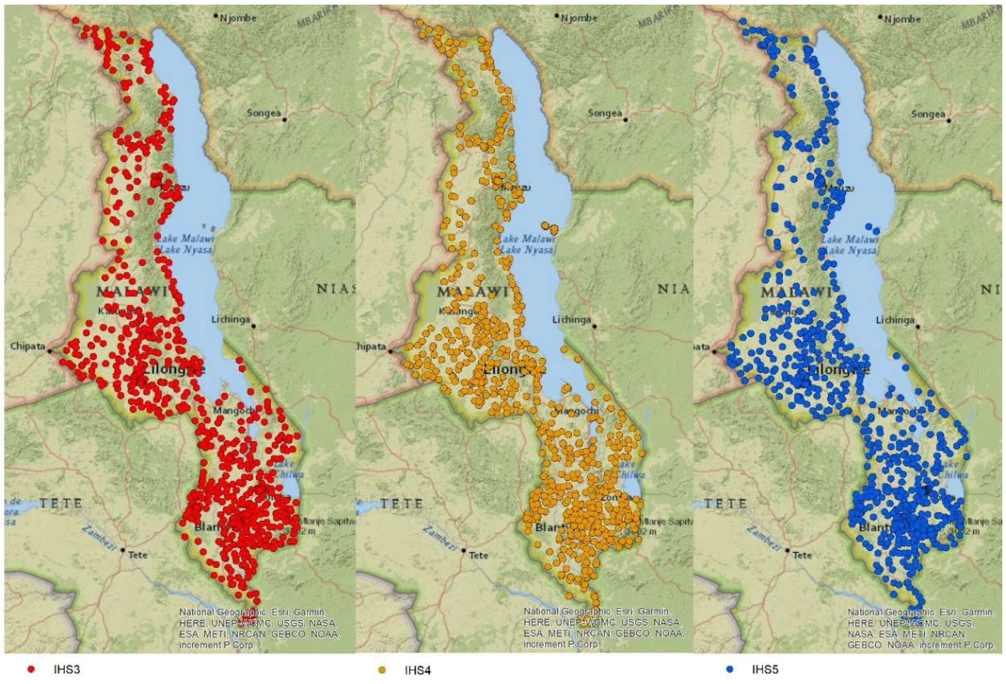
The study uses data from multiple rounds of Malawi’s rich and nationally representative Integrated Household Survey (IHS). We precisely work with the three latest rounds collected for the 2011 (IHS3), 2016 (IHS4), and 2018 (IHS5) agricultural seasons that captured elaborated information on commercial input purchasing decisions. The survey data are available through the Living Standards Measurement Study–Integrated Surveys on Agriculture (LSMS–ISA) program of the World Bank in collaboration with the government of Malawi. The LSMS–ISA data collect comprehensive information on agricultural activities, household perceptions of shock exposure in the recent past, various farm and household socioeconomic conditions, and georeferenced data, which we use to extract spatial climate data and derive objective measures of climate shocks. The distribution of enumeration areas (villages) included in the three rounds of the Malawi survey data is shown in Figure 3. The surveys cover the entire country and the collected samples are representative of the three main geographic regions in Malawi (northern, central, and southern regions) and can be used to answer this study’s research questions. Households are the primary units of observation analyzed in this study. The IHS3, IHS4, and IHS5 cover 12,271, 12,447, and 11,434 households, of which the majority (more than 80%) are rural agricultural households involved in agricultural production activities. Our analysis is based on these rural households with complete and usable information on input acquisition and mainly agricultural input purchasing activities (fertilizers, agrochemicals, seeds, and labor). The combined sample we analyze comprises 25,631 rural households shared as 16, 35, and 49% between the northern, central, and southern regions.

4.1.2. Rainfall and Temperature Data

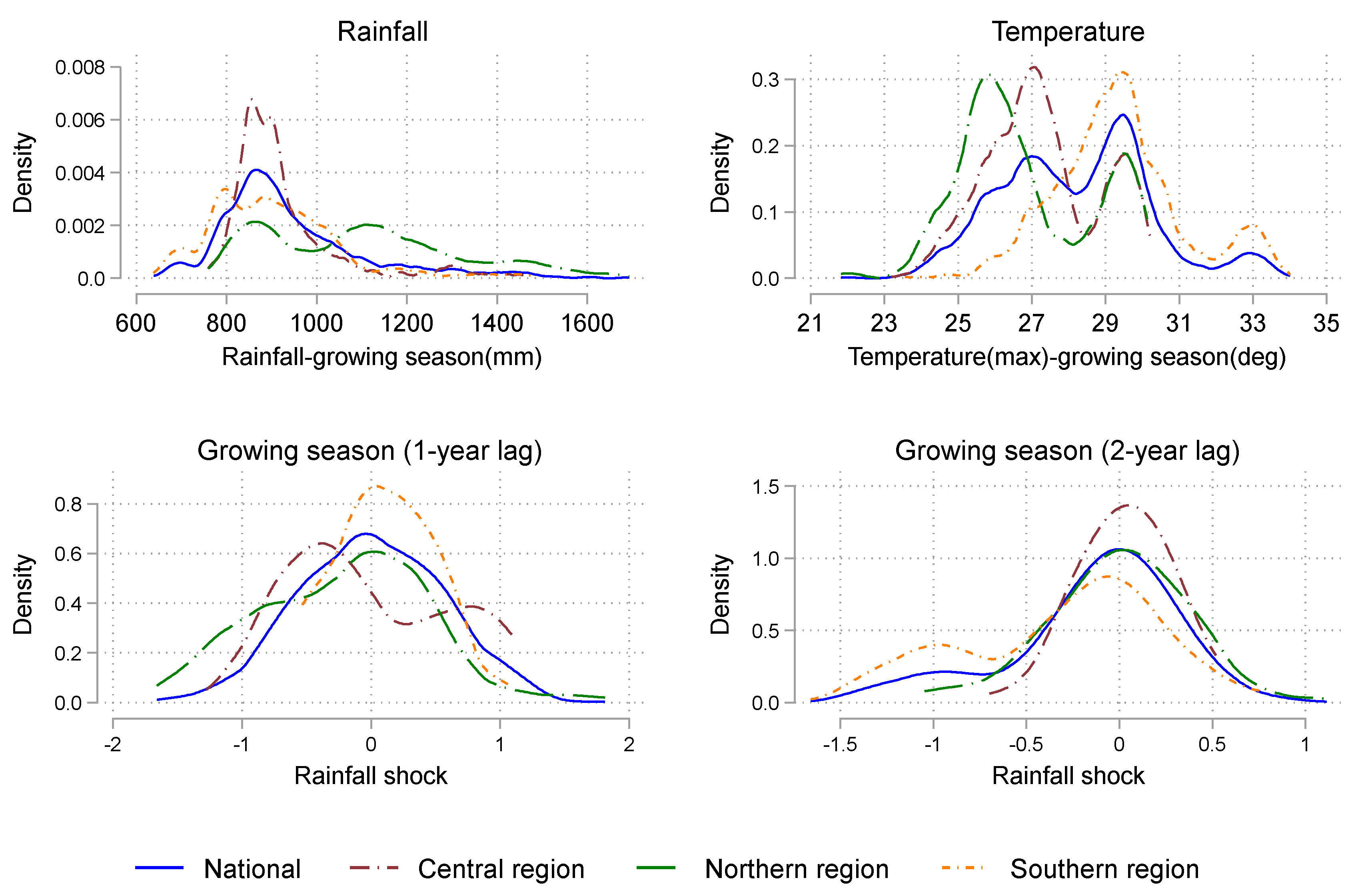
In addition to the LSMS–ISA household data, we extract historical monthly weather data from WorldClim [55] for 39 years using georeferenced data (longitude and latitude) available with the LSMS–ISA household data. We use the extracted rainfall and temperature data to define our objective measures of climate risk variables, including lagged droughts and flood shocks. All climate risk variables used in the analysis are defined for Malawi’s main crop growing season, spanning from November to April. In Figure 4, we plot the distribution of rainfall and maximum temperature in the analyzed sample and three main regions in Malawi. In addition to the long-term averages for climate, we define rainfall shocks. We define lagged rainfall shock variables as normalized deviations in a single season’s rainfall from the seasonal rainfall variable over a reference period (39-year average). We define a rainfall shock (${\mathrm{Rainshock}}_{\mathrm{E}\mathrm{t}}$) at time t in a particular season (growing season) as follows: ${\mathrm{Rainshock}}_{\mathrm{Et}}=\left\{\frac{{\mathrm{R}}_{\mathrm{Et}}-\widehat{{\mathrm{R}}_{\mathrm{E}}}}{{\mathsf{\sigma }}_{{\mathrm{R}}_{\mathrm{E}}}}\right\}$, where: ${\mathrm{R}}_{\mathrm{E}\mathrm{t}}$ is the observed amount of rainfall for the season and $\widehat{{\mathrm{R}}_{\mathrm{E}}}, {\mathsf{\sigma }}_{{\mathrm{R}}_{\mathrm{E}}}$ are, respectively, the long-term average seasonal rainfall and standard deviation. Consequently, the resultant rainfall shock (Z-score) will consist of positive and negative Z-scores. The negative (positive) Z-scores show the extent to which rainfall in a particular season was below (above) the long-term average. We define drought and flood shocks as negative and positive Z-scores, respectively.

We plot the distribution of rainfall shock measures in the past two seasons (1-year and 2-year lags) in the pooled sample and by region in Figure 4.

4.2. Model Specification and Empirical Estimation

4.2.1. Model Specification

Smallholder farmers make input purchase decisions in a two-step process: first, they decide whether to purchase a particular input or not and, second, to what extent (quantity or value of the purchase). We model input purchasing decisions using suitable limited dependent variable models [26]. The models assume that the choice between alternatives (purchasing and non-purchasing) depends on identifiable characteristics. The decision-maker (the farmer) is also believed to maximize the expected utility from the decision (choices) they make subject to constraints [56]. In the context of climate shocks, farmers are expected to choose input purchases that maximize the anticipated utility of returns under different states of nature (with and without shocks) [24]. Given the inseparable nature of production and consumption decisions, input purchase functions are based on consumption and production characteristics. We, therefore, model input purchasing as given in the equation below:

$$C_{ik}={\theta }_0+{\theta }_{1}Climat{e}_p+{\theta }_2{H}_i+{\theta }_{3}Y{D}_i+{\epsilon }_i$$

(1)

where $C_{ik}=$ is the dependent variable, which represents different values for purchase (1 = yes: 0 otherwise) and intensity of purchase (quantity or value purchased/ha) for specific input $k$ (fertilizer, agrochemicals, labor, or seed); $Climate$ = vector of climate risk variables; $H_i$ = vector of household socioeconomic variables (elaborated below); $YD$ = survey year dummies and regional variables; and ${\epsilon }_i$ = random error term. The climate risk vector includes rainfall shocks (drought and flood) and long-term climate variables (rainfall and temperature) for the crop growing season. These are our primary variables of interest. We focus on specific drought and flood shocks, which measure the exposure and intensity of exposure to negative and positive normalized rainfall deviations, respectively. In the vector ($H_i$) we include other control variables commonly included in technology adoption studies [19,20], including farm size (ha), number of plots cultivated by the household, family labor (days), household wealth index (we use a collection of household assets, housing dwelling characteristics, and household access to basic services (e.g., clean water, energy, and sanitation) available in the Malawi LSMS–ISA data to compute a household wealth index using Principal Components Analysis [57]), agricultural implement access index (we summarize information on a household’s ownership of various agricultural equipment and tools available in the Malawi LSMS–ISA data using PCA to derive an index that we term as agricultural implements access index), dummy variables for access to fertilizer and seed coupons, distance to the nearest Agricultural Development and Marketing Corporation (ADMARC) center (km), household size, household dependency ratio (the household dependency ratio is a ratio (expressed as a percentage) of economically active household members (≥15 years and less than 65) to household dependency (<15 years and >65 years)), and characteristics of the household head (gender, age, education). In addition, we also control for district-level dummies and survey year dummies. We present descriptive statistics of these variables in the Supplementary Materials (Table S1).

4.2.2. Estimation Strategy

We estimate parameters in Equation (1) using Cragg’s Double-Hurdle (DH) models [58], which allows us to specify separate hurdles for the probability of input purchase (Hurdle 1) and the intensity of purchase for purchasers (Hurdle 2). An alternative would have been to use the Tobit Model [59] for input purchase decisions. However, the Tobit model is statistically restrictive, as it assumes that the same set of variables equally determines both the probability of non-zero input purchase and the intensity of purchase, which might not always be the case. The double-hurdle (DH) model, proposed initially by Cragg [58], overcomes the restrictive assumptions of the Tobit model and assumes that individual farmers make two decisions concerning the choice and extent of an input purchase. We hence apply the DH models to study input purchase decisions in this study. Within the DH model, the first Hurdle (the probability of input purchase for a specific input) is estimated using a probit estimator and the second Hurdle (intensity of purchase decision) is estimated using a truncated normal regression model that accounts for those who do not purchase a particular input [26,58]. We follow the recommendations in Burke [60] and estimate the first and second hurdles of the Craggit model simultaneously to improve efficiency in the estimation. We estimate parameters in Equation (1) first for a general model of investment and the extent of investment in purchased inputs followed by models of specific inputs purchased (fertilizer, agrochemicals, labor, and seed).

In addition to the main results, we also aim to perform a heterogeneity analysis. We primarily explore how differences in regional settings may potentially influence the relationships between climate risk exposure and the need for commercially purchased inputs. Second, we explore how differential resource endowments (land and non-land assets), access to information, and the gender of household leaders influence household responses to shocks through input purchasing. To assess for possible regional heterogeneities in the influence of climate risk on input purchasing, we estimate separate models for the three main regions in Malawi (northern, central, and southern regions). We do this by splitting our samples into the three regions (northern, central, and southern regions) and estimating (Equation (1)) for specific inputs in the respective sub-samples. We specify separate equations for each geographic region (R = 1, 2, or 3) as follows:

$$C_{ik}^R={\beta }_0+{\beta }_{1}Climat{e}_p+{\beta }_2{H}_i+{\beta }_{3}Y{D}_i+{ϵ}_i$$

(2)

where parameters are as described earlier and the superscript $R$ takes different values for specific regions studied (R = 1, 2, and 3 for northern, central, and southern regions, respectively). Furthermore, to explore heterogeneity in the impact of shocks on input purchasing between the poor and the rich (based on asset endowments), we do the following: (i) first, estimate a composite score of household wealth endowments based on their total landholding, agricultural assets owned, and ownership of durable household assets as previously explained, (ii) make two quintiles of household wealth endowments that distinguish better-endowed households (quintile 2), and poorly endowed households (quintile 1), and (iii) estimate Equation (1) in sub-samples of poorer and richer households as in Equation (3):

$$C_{ik}^Q={\beta }_0+{\beta }_{1}Climat{e}_p+{\beta }_2{H}_i+{\beta }_{3}Y{D}_i+{ϵ}_i$$

(3)

where parameters are as described earlier and the superscript $Q$ takes different values for different quintiles of asset wealth (1 = poorer and 2 = richer households). Similarly, we explore possible gender and access to information heterogeneities in results by estimating Equation (1) in sub-samples of gender (male and female-led households) and information access (yes or no access), respectively. We proxy access to agricultural information by a dummy variable measuring access to agricultural extension services from various sources (government and private sources) and on various topics including input access and use. To gain additional insights from the analysis of possible gender differences, we explore heterogeneity analysis by marital status and wealth endowment categories of male and female household heads. By doing so, we can further illuminate some unobserved covariates related to household heads’ marital statuses that the gender coefficient might capture. For instance, female-led households are usually led by single women (e.g., widowed or divorced) who are poor and have disadvantaged positions in traditional society [50,61,62]. In estimating our models, we correct standard errors by specifying clustering at the primary sampling unit (village) to correct any potential intra-cluster correlation of climate risk variables. We report marginal effects to help with the economic interpretation of results. For the first hurdle (probit model), we report marginal effects ($E[Y|X])$, and conditional marginal effects ($E\left[Y|X\right], if Y>0)$ for the second hurdle (truncated regression model). In addition to the results presented in tables, we also plot average partial effects on the relationships between our dependent variables and key explanatory variables (climate variables and shocks) to provide visuals of the key relationships found.

We also perform sensitivity analysis to assess the robustness of our main results. We mainly perform robustness analysis by estimating parsimonious models of input purchasing with only key variables of interest (climate risk variables) first and then assess how adding control variables (vector $H_i$) alter our conclusions. In all our estimations, the addition of additional controls to parsimonious specifications does not alter our conclusions. We are confident that our estimates are robust to the addition of additional control variables. In addition to the analysis, we define subjective measures of household rainfall shock exposure using perception data available in the LSMS–ISA household data. The Malawi LSMS–ISA data captures household perceptions of shock experienced in the recent past, which can be used to define drought, floods, and other shock experiences. We test the influence of rainfall shocks using these data to assess whether commercial input purchases respond to these shocks. We reproduce the main tables shown in the manuscript by replacing objective measures of drought and flood shocks defined by the historical climate data with subjective measures of drought and flood shocks defined by household perceptions. We report the results in the Supplementary Materials, which confirm rainfall shocks (perceptions) as significant determinants for commercial input purchases across regions.

4.2.3. Study Limitations

Our study is not without limitations. We rely on secondary (self-reported) data of farmer input purchasing decisions that could be associated with recall bias and other related errors. Additionally, we work on the assumption that rainfall deviation from a long-term average in specific clusters across regions is purely random, which might be a strong assumption in some cases. Despite the noted limitations, our paper adds important insights to the literature on the possible influence of climate risk factors in driving demand for key off-farm and productivity improving inputs in heterogeneous settings.

5. Results

5.1. Descriptive Statistics

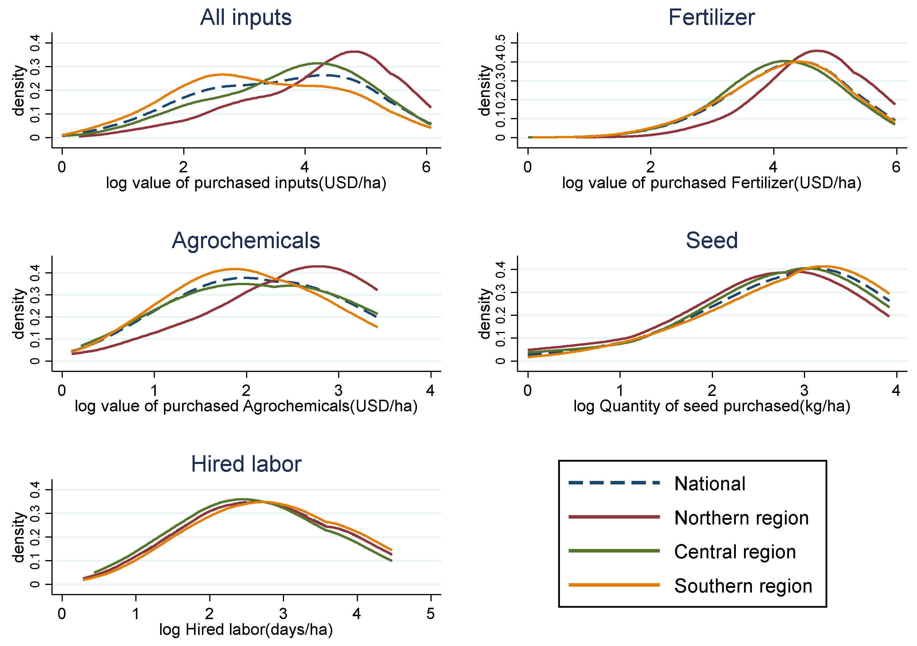
We present descriptive statistics of our key outcome and explanatory variables of interest using a combination of tables and figures in the pooled (national) sample and by the three main regions studied. For brevity, we comment only on our key outcome variables. Table 1 presents descriptive statistics for input purchasing variables by region and survey years. In general, we can tell that about 59% of farmers purchased inputs (either agrochemicals, seed, or fertilizer) in the national sample and that input purchasing has increased over time (from 43 to 71% from IHS3 to IHS5). Similarly, about 49% of farmers used purchased inputs in the northern region, with purchasing rates increasing from IHS3 to IHS5 by 23% (from 32 to 55%). The central region has slightly higher rates of input purchasing, with about 61% of farmers indicating to have used purchased inputs. In addition, rates of input purchasing have increased from 44% to 75% from IHS3 to IHS5 in the central region. The southern region has almost the same rates for input purchasing as the central region, with about 60% of farmers indicating to have used purchased inputs and a 29% increase in that rate from IHS3 to IHS5. Although the northern region has comparably lower rates of purchasing inputs, they have the highest average for the amount spent on input purchasing (Table 1 and Figure 5). We also show the distributions of input purchasing intensity in general and the three regions in Figure 5.

We also report purchasing rates and intensity of purchase for specific inputs. For fertilizer, we see that in the national sample, about 39% of farmers purchased inorganic fertilizer and that over time rates show an increasing trend from 33% (IHS3) to 45% (IHS5). Comparing fertilizer input purchasing rates by region show that the average rates of using purchased fertilizer are highest in the central region (49%) and lowest in the southern region (29%). The northern region has about 43% of farmers reporting to have used purchased inorganic fertilizers (Table 1). Assessing trends over time, we also see that the rate of using purchased fertilizer has increased from IHS3 to IHS5 by 12, 6, 9, and 17% in the national, northern, central, and southern region samples, respectively. In terms of the intensity of fertilizer purchasing, the northern region has comparably higher intensities of fertilizer purchasing than other regions (Table 1 and Figure 5).

Regarding agrochemical purchasing, we see low rates of agrochemical use in national samples and in given regions. On average, about 4% of studied farmers purchased agrochemicals in the national sample. The rate of purchasing agrochemicals in the national sample increased slightly from IHS3 to IHS5 from 2 to 6%. In the northern region, on average, 4% of farmers purchased agrochemicals and the purchase rate increased by 3% from IHS3 (2%) to IHS5 (5%). Likewise, on average, 3% of farmers purchased agrochemicals in the central region and from IHS3 to IHS5, the rate of using purchased agrochemicals rose from 4 to 7%. Likewise, about 4% of farmers in the southern region purchased agrochemicals. The farmers purchasing agrochemicals in the southern region rose from 3% in IHS3 to 5% in IHS5 (Table 1). We show the distribution of agrochemical purchase intensities in the national sample and the three main regions of Malawi in Figure 6. In purchasing intensity, we again see that the northern region has a comparably higher intensity of purchasing agrochemicals than other regions (Figure 5 and Table 1).

Table 1. Descriptive statistics of outcome variables by survey round.

	National				Northern Region				Central Region				Southern Region
	Full	IHS3	IHS4	IHS5	Full	IHS3	IHS4	IHS5	Full	IHS3	IHS4	IHS5	Full	IHS3	IHS4	IHS5
Variables	Mean	Mean	Mean	Mean	Mean	Mean	Mean	Mean	Mean	Mean	Mean	Mean	Mean	Mean	Mean	Mean
Outcome variables (input purchasing)
Input purchase (in general)
Purchased any inputs (1 = yes)	0.587	0.427	0.644	0.714	0.490	0.317	0.623	0.548	0.609	0.443	0.659	0.750	0.604	0.452	0.641	0.740
Value of purchased inputs (USD/ha)	73.993	86.384	65.994	73.175	120.220	140.831	107.997	121.688	78.324	102.529	67.308	71.995	58.495	61.996	51.163	62.861
Inorganic Fertilizer
Purchased inorganic fertilizer (1 = yes)	0.379	0.331	0.362	0.454	0.425	0.380	0.459	0.439	0.485	0.456	0.456	0.549	0.288	0.224	0.262	0.391
Value of purchased fertilizer (USD/ha)	100.542	128.357	92.289	90.674	137.393	175.159	124.842	127.716	89.765	119.295	80.095	77.683	96.592	119.757	88.408	90.763
Agrochemicals (herbicide or pesticide)
Purchased agrochemicals (herbicides or pesticide) (1 = yes)	0.036	0.023	0.026	0.060	0.035	0.025	0.030	0.053	0.034	0.014	0.018	0.074	0.037	0.028	0.031	0.053
Value of purchased agrochemicals (USD/ha)	10.726	9.137	9.662	11.901	14.451	16.978	14.156	13.907	11.130	11.391	8.946	11.734	9.405	7.058	8.413	11.447
Seed (in at least one of the crops grown)
Purchased seed (1 = yes)	0.472	0.404	0.490	0.533	0.363	0.302	0.436	0.354	0.446	0.369	0.447	0.534	0.527	0.465	0.539	0.587
Value of purchased seeds (USD/ha)	17.750	18.750	16.994	17.833	22.796	18.548	22.721	25.603	18.110	20.129	16.374	18.467	16.471	18.068	15.784	15.974
Quantity of seeds purchased (kg/ha)	21.256	19.612	20.831	22.779	17.525	13.087	18.398	19.055	19.724	18.657	18.980	21.008	22.958	21.157	22.594	24.634
Labor (hired paid labor)
Hired labor (1 = yes)	0.173	0.158	0.168	0.196	0.171	0.126	0.174	0.225	0.186	0.189	0.188	0.182	0.164	0.146	0.152	0.197
Hire labor (days)	22.833	19.798	24.184	24.436	23.223	14.546	25.572	27.141	20.179	19.521	22.138	18.819	24.872	21.581	25.448	27.207
Number of observations	25,631	9207	8551	7873	4123	1502	1415	1206	9001	3245	2969	2787	12,507	4460	4167	3880

Notes: Source: authors own elaboration based on Malawi LSMS–ISA data. We converted the value of purchased inputs from local currency (MWK) to USD to enable comparison of the intensity of purchase across surveys years. We use average exchange rates for specific survey years available on Google (https://www.exchangerates.org.uk/, accessed on 7 September 2022). For example, we use specific exchange rates for the different survey years IHS3 (https://www.exchangerates.org.uk/USD-MWK-spot-exchange-rates-history-2010.html), IHS4 (https://www.exchangerates.org.uk/USD-MWK-spot-exchange-rates-history-2016.html), and IHS5 (https://www.exchangerates.org.uk/USD-MWK-spot-exchange-rates-history-2019.html), accessed on 7 September 2022.

Table 1. Descriptive statistics of outcome variables by survey round.

	National				Northern Region				Central Region				Southern Region
	Full	IHS3	IHS4	IHS5	Full	IHS3	IHS4	IHS5	Full	IHS3	IHS4	IHS5	Full	IHS3	IHS4	IHS5
Variables	Mean	Mean	Mean	Mean	Mean	Mean	Mean	Mean	Mean	Mean	Mean	Mean	Mean	Mean	Mean	Mean
Outcome variables (input purchasing)
Input purchase (in general)
Purchased any inputs (1 = yes)	0.587	0.427	0.644	0.714	0.490	0.317	0.623	0.548	0.609	0.443	0.659	0.750	0.604	0.452	0.641	0.740
Value of purchased inputs (USD/ha)	73.993	86.384	65.994	73.175	120.220	140.831	107.997	121.688	78.324	102.529	67.308	71.995	58.495	61.996	51.163	62.861
Inorganic Fertilizer
Purchased inorganic fertilizer (1 = yes)	0.379	0.331	0.362	0.454	0.425	0.380	0.459	0.439	0.485	0.456	0.456	0.549	0.288	0.224	0.262	0.391
Value of purchased fertilizer (USD/ha)	100.542	128.357	92.289	90.674	137.393	175.159	124.842	127.716	89.765	119.295	80.095	77.683	96.592	119.757	88.408	90.763
Agrochemicals (herbicide or pesticide)
Purchased agrochemicals (herbicides or pesticide) (1 = yes)	0.036	0.023	0.026	0.060	0.035	0.025	0.030	0.053	0.034	0.014	0.018	0.074	0.037	0.028	0.031	0.053
Value of purchased agrochemicals (USD/ha)	10.726	9.137	9.662	11.901	14.451	16.978	14.156	13.907	11.130	11.391	8.946	11.734	9.405	7.058	8.413	11.447
Seed (in at least one of the crops grown)
Purchased seed (1 = yes)	0.472	0.404	0.490	0.533	0.363	0.302	0.436	0.354	0.446	0.369	0.447	0.534	0.527	0.465	0.539	0.587
Value of purchased seeds (USD/ha)	17.750	18.750	16.994	17.833	22.796	18.548	22.721	25.603	18.110	20.129	16.374	18.467	16.471	18.068	15.784	15.974
Quantity of seeds purchased (kg/ha)	21.256	19.612	20.831	22.779	17.525	13.087	18.398	19.055	19.724	18.657	18.980	21.008	22.958	21.157	22.594	24.634
Labor (hired paid labor)
Hired labor (1 = yes)	0.173	0.158	0.168	0.196	0.171	0.126	0.174	0.225	0.186	0.189	0.188	0.182	0.164	0.146	0.152	0.197
Hire labor (days)	22.833	19.798	24.184	24.436	23.223	14.546	25.572	27.141	20.179	19.521	22.138	18.819	24.872	21.581	25.448	27.207
Number of observations	25,631	9207	8551	7873	4123	1502	1415	1206	9001	3245	2969	2787	12,507	4460	4167	3880

Notes: Source: authors own elaboration based on Malawi LSMS–ISA data. We converted the value of purchased inputs from local currency (MWK) to USD to enable comparison of the intensity of purchase across surveys years. We use average exchange rates for specific survey years available on Google (https://www.exchangerates.org.uk/, accessed on 7 September 2022). For example, we use specific exchange rates for the different survey years IHS3 (https://www.exchangerates.org.uk/USD-MWK-spot-exchange-rates-history-2010.html), IHS4 (https://www.exchangerates.org.uk/USD-MWK-spot-exchange-rates-history-2016.html), and IHS5 (https://www.exchangerates.org.uk/USD-MWK-spot-exchange-rates-history-2019.html), accessed on 7 September 2022.

The descriptive statistics for the use of purchased seeds are also given in Table 1 and Figure 5. Seed purchasing is found to be a common practice in the national sample and all regions. On average, 47, 36, 45, and 53% of farmers in the national sample, northern, central, and southern regions, used commercially purchased seeds. Assessing trends over time (between his3 ahisIHS5) using purchased seeds in national, northern, central, and southern regions increased by 13, 5, 16, and 12%, respectively (Table 1). We report average seed purchasing intensities in their quantities and the value of seeds purchased in Table 1. We also show the distribution of seed purchasing intensities in the national sample and by region in Figure 6. We observe comparable seed purchasing intensities in all three regions with slightly higher intensities in the southern region (in quantities of seeds purchased/ha) compared to other regions on average (Figure 5).

Regarding the use of hired labor, we see that, on average, between 17 and 19% of the farmers in the national sample and three regions use hired labor. Assessing the trends over time shows us that the northern region had the largest surge in the use of hired labor, from 12 to 23% between IHS3 and IHS5. The national sample and the southern region also show a slight increase in the use of hired labor from 16–20% and 15–20%, respectively. On the contrary, hired labor slightly fell from 19% in IHS3 to 18% in IHS5 in the central region (Table 1). We also present the average number of days of hired labor use in the national sample and by region in Table 1. In addition, we also show the distribution of the number of hired labor (log-transformed) days in the national sample and by region in Figure 5. We see fairly similar patterns in the distribution of hired labor use intensities in the national sample and the studied regions.

When we compare input purchasing variables (purchase and intensity of purchase) by household wealth endowment quintiles, access to information, and the gender of household heads, we learn that input purchase rates and intensities are higher amongst richer, informed, and male headed-households compared to their counterparts (poorer, not informed, and female-headed households) (the results are summarized in the Supplementary Materials, in Figures S1–S31 and Tables S1–S2).

5.2. Impact of Climate Risk on Input Purchasing Decisions in Different Regions in Malawi

This section presents results showing the influence of rainfall shocks on input purchasing decisions. We start by reporting results from a general model of input purchasing and then move on to models of specific inputs purchased, including inorganic fertilizer, agrochemicals, seed, and hired labor. We present one table of results for each model in Table 2, Table 3, Table 4, Table 5 and Table 6. In addition to the tables, we plot the marginal effects of key explanatory variables that visualize the relationship between climate risk variables and input purchase decisions from general input purchase to labor hire (Figure 6, Figure 7, Figure 8, Figure 9 and Figure 10).

5.2.1. Investment in Commercial Inputs (in a General Model)

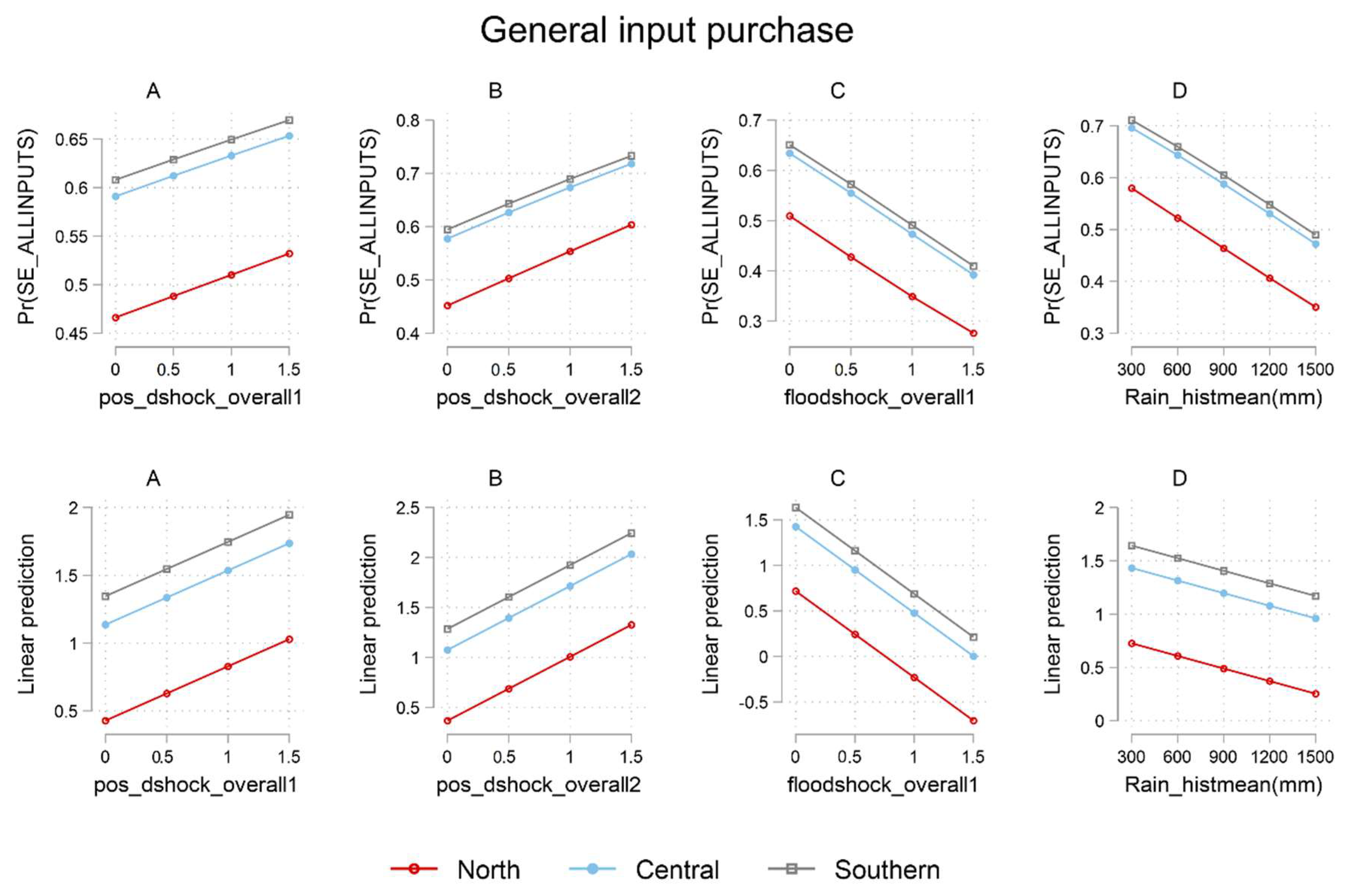
Table 2 reports results from a general model that considers whether a farmer purchased any input (fertilizer, agrochemicals, or seed). From the results, a 1-year lag drought shock enhances input purchasing in the national sample, the central region, and the southern regions (Table 2). A 2-year lag drought shock enhances the likelihood of purchasing inputs in the national sample and the central region but reduces the intensity of input purchase in the northern region (Table 2). Regarding flood shocks, we see that a one-year lag of flood shock reduces the likelihood of purchasing inputs but enhances the intensity of purchase for purchasers in the national sample and all regions (Table 2). Additionally, we learn that long-term average seasonal rainfall enhances input purchasing decisions in the national sample and across all regions and that the long-term average growing season temperatures reduce input purchasing decisions in the national sample and across regions (Table 2).

Table 2. The influence of rainfall shocks on input purchasing (general) across regions in Malawi.

	National		Northern		Central		Southern
VARIABLES	Hurdle1	Hurdle2	Hurdle1	Hurdle2	Hurdle1	Hurdle2	Hurdle1	Hurdle2
Climate risk variables
Growing season drought shock (1-year lag)	0.059 *** (0.0221)	0.078 (0.0645)	0.033 (0.0411)	−0.018 (0.1200)	0.041 (0.0403)	0.200 * (0.1213)	0.120 ** (0.0612)	0.662 *** (0.2118)
Growing season drought shock (2-year lag)	0.102 *** (0.0216)	0.011 (0.0630)	−0.018 (0.0598)	−0.539 ** (0.2167)	0.226 ** (0.0902)	0.630 ** (0.2798)	0.047 (0.0487)	−0.164 (0.1379)
Growing season flood shock (1-year lag)	−0.155 *** (0.0253)	0.278 *** (0.0630)	−0.020 (0.0428)	0.494 *** (0.1093)	−0.286 *** (0.0435)	−0.052 (0.1376)	−0.280 *** (0.0526)	0.266 ** (0.1308)
Long-term season average rainfall (mm)	0.000 ** (0.0001)	0.002 *** (0.0004)	0.000 (0.0002)	0.001 ** (0.0006)	0.000 (0.0003)	0.002 ** (0.0007)	0.001 ** (0.0002)	0.001 ** (0.0007)
Long-term season average temperature (deg)	−0.014 *** (0.0050)	−0.180 *** (0.0134)	0.004 (0.0141)	−0.090 *** (0.0346)	−0.030 *** (0.0080)	−0.182 *** (0.0226)	−0.009 (0.0064)	−0.187 *** (0.0187)
Other control variables	Yes	Yes	Yes	Yes	Yes	Yes	Yes	Yes
Sigma constant		1.139 *** (0.0078)		1.094 *** (0.0216)		1.119 *** (0.0126)		1.153 *** (0.0112)
Survey year dummies	Yes	Yes	Yes	Yes	Yes	Yes	Yes	Yes
District fixed effects	Yes	Yes	Yes	Yes	Yes	Yes	Yes	Yes
Observations	25,631	15,058	4123	2019	9001	5484	12,502	7555

Notes: Cluster robust standard errors with clustering specified at the primary sampling unit are in parenthesis. Hurdle 1 is a probit regression for the probability of input purchase while Hurdle 2 is the model for intensity of purchase for purchasers (log value of purchased inputs (USD/ha), * p < 0.10, ** p < 0.05, *** p < 0.01. Input purchasing is defined in general (fertilizer, agrochemicals, or seed).

Table 2. The influence of rainfall shocks on input purchasing (general) across regions in Malawi.

	National		Northern		Central		Southern
VARIABLES	Hurdle1	Hurdle2	Hurdle1	Hurdle2	Hurdle1	Hurdle2	Hurdle1	Hurdle2
Climate risk variables
Growing season drought shock (1-year lag)	0.059 *** (0.0221)	0.078 (0.0645)	0.033 (0.0411)	−0.018 (0.1200)	0.041 (0.0403)	0.200 * (0.1213)	0.120 ** (0.0612)	0.662 *** (0.2118)
Growing season drought shock (2-year lag)	0.102 *** (0.0216)	0.011 (0.0630)	−0.018 (0.0598)	−0.539 ** (0.2167)	0.226 ** (0.0902)	0.630 ** (0.2798)	0.047 (0.0487)	−0.164 (0.1379)
Growing season flood shock (1-year lag)	−0.155 *** (0.0253)	0.278 *** (0.0630)	−0.020 (0.0428)	0.494 *** (0.1093)	−0.286 *** (0.0435)	−0.052 (0.1376)	−0.280 *** (0.0526)	0.266 ** (0.1308)
Long-term season average rainfall (mm)	0.000 ** (0.0001)	0.002 *** (0.0004)	0.000 (0.0002)	0.001 ** (0.0006)	0.000 (0.0003)	0.002 ** (0.0007)	0.001 ** (0.0002)	0.001 ** (0.0007)
Long-term season average temperature (deg)	−0.014 *** (0.0050)	−0.180 *** (0.0134)	0.004 (0.0141)	−0.090 *** (0.0346)	−0.030 *** (0.0080)	−0.182 *** (0.0226)	−0.009 (0.0064)	−0.187 *** (0.0187)
Other control variables	Yes	Yes	Yes	Yes	Yes	Yes	Yes	Yes
Sigma constant		1.139 *** (0.0078)		1.094 *** (0.0216)		1.119 *** (0.0126)		1.153 *** (0.0112)
Survey year dummies	Yes	Yes	Yes	Yes	Yes	Yes	Yes	Yes
District fixed effects	Yes	Yes	Yes	Yes	Yes	Yes	Yes	Yes
Observations	25,631	15,058	4123	2019	9001	5484	12,502	7555

Notes: Cluster robust standard errors with clustering specified at the primary sampling unit are in parenthesis. Hurdle 1 is a probit regression for the probability of input purchase while Hurdle 2 is the model for intensity of purchase for purchasers (log value of purchased inputs (USD/ha), * p < 0.10, ** p < 0.05, *** p < 0.01. Input purchasing is defined in general (fertilizer, agrochemicals, or seed).

Figure 6. Plotting marginal effects of changes in 1-year lag drought shocks (pos_dshock_overall1), 2-year lag drought shock (pos_dshock_overall2), 1-year lag flood shock (floodshock_overall1), and historical mean rainfall (Rain_histmean (mm)) on the probability (top panel), and intensity of input purchase (bottom panel) by region.

Figure 6. Plotting marginal effects of changes in 1-year lag drought shocks (pos_dshock_overall1), 2-year lag drought shock (pos_dshock_overall2), 1-year lag flood shock (floodshock_overall1), and historical mean rainfall (Rain_histmean (mm)) on the probability (top panel), and intensity of input purchase (bottom panel) by region.

From the general model of input purchasing, we learn the general effects of climate risk variables on input purchasing. However, given that input purchasing practices for specific inputs vary across regions and that climate risk variables could prompt different input purchasing responses for specific inputs, the general model may not provide us with accurate information on the relationships. Therefore, in the following sections, we report results from models of purchasing practices for specific inputs.

5.2.2. Inorganic Fertilizers

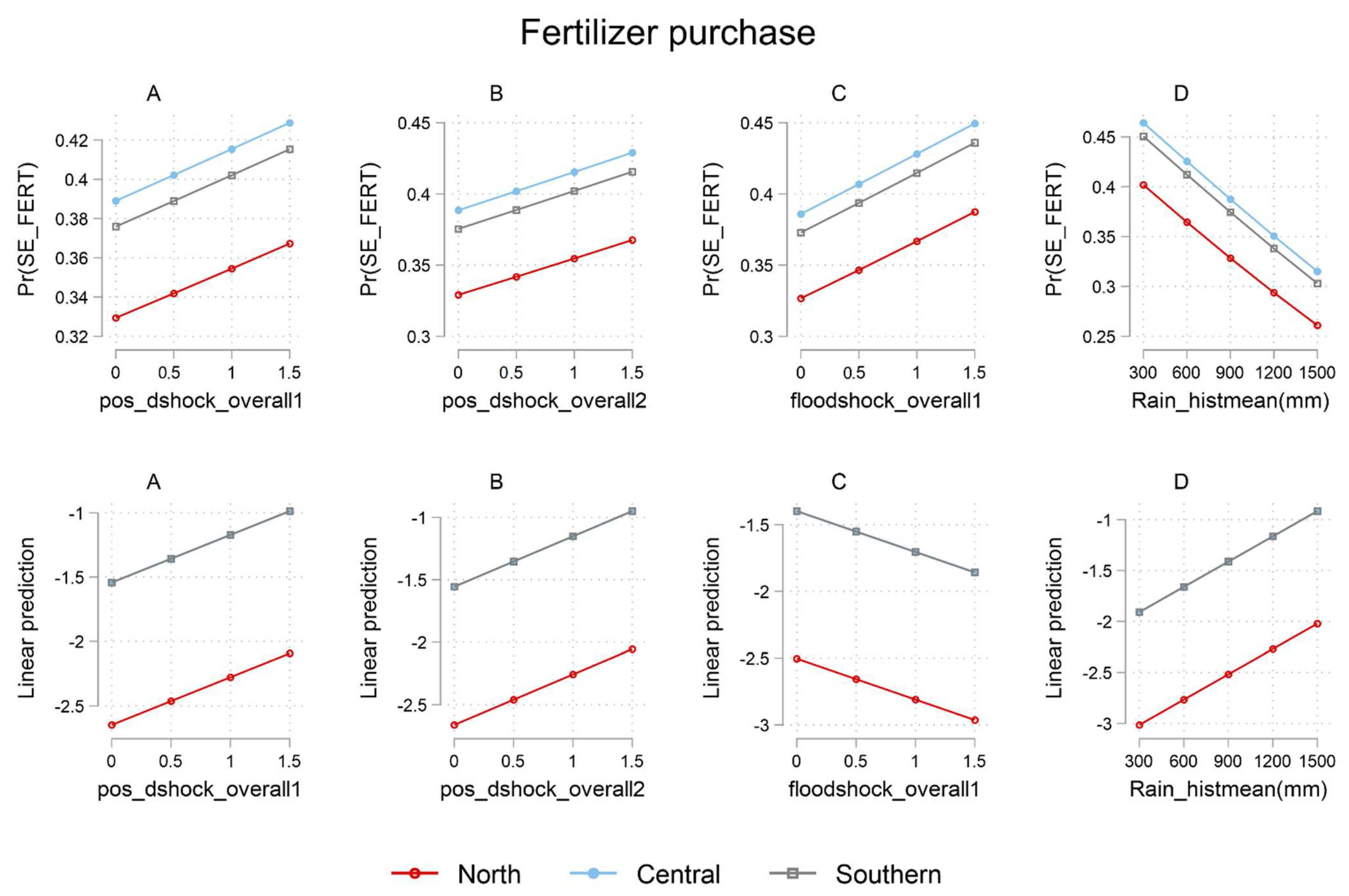
In Table 3, we present results on the impact of rainfall shocks on purchasing inorganic fertilizers. From the results, we learn that exposure to the 1-year lag of drought shock enhances the intensity of fertilizer purchasing in the central and southern regions. Additionally, the 2-year lag of drought shock exposure enhances the likelihood of purchasing fertilizer in the national sample, enhances the likelihood and intensity of purchasing fertilizer in the central region, and reduces the chances of purchasing fertilizer in the northern and southern regions (Table 3).

Regarding flood shocks, we learn that a 1-year lag enhances the intensity of fertilizer purchases in the northern region and reduces the intensity of fertilizer purchases in the central region. In addition, long-term rainfall enhances fertilizer purchases, while temperature discourages fertilizer purchases in the national sample and studied regions (Table 3).

Table 3. The influence of rainfall shocks on fertilizer purchasing across regions in Malawi.

	National		Northern		Central		Southern
VARIABLES	Hurdle1	Hurdle2	Hurdle1	Hurdle2	Hurdle1	Hurdle2	Hurdle1	Hurdle2
Climate risk variables
Growing season drought shock (1-year lag)	0.032 (0.0198)	0.054 (0.0481)	−0.037 (0.0364)	0.089 (0.0851)	0.051 (0.0395)	0.223 ** (0.0948)	0.062 (0.0609)	0.636 *** (0.1712)
Growing season drought shock (2-year lag)	0.070 *** (0.0197)	0.046 (0.0549)	−0.113 ** (0.0530)	−0.142 (0.1739)	0.178 ** (0.0843)	0.548 ** (0.2172)	−0.119 *** (0.0423)	0.146 (0.1419)
Growing season flood shock (1-year lag)	0.013 (0.0170)	0.060 (0.0521)	0.051 (0.0378)	0.232 ** (0.0924)	0.029 (0.0363)	−0.234 ** (0.1029)	0.006 (0.0343)	0.104 (0.1283)
Long-term season average rainfall (mm)	0.000 (0.0001)	0.002 *** (0.0003)	0.000 (0.0002)	0.002 *** (0.0005)	0.000 (0.0002)	0.001 ** (0.0006)	0.000 (0.0002)	0.001 (0.0007)
Long-term season average temperature (deg)	−0.051 *** (0.0042)	−0.097 *** (0.0102)	−0.020 * (0.0110)	−0.065 *** (0.0204)	−0.051 *** (0.0077)	−0.094 *** (0.0167)	−0.058 *** (0.0050)	−0.101 *** (0.0149)
Other control variables	Yes	Yes	Yes	Yes	Yes	Yes	Yes	Yes
Sigma constant		0.821 *** (0.0079)		0.751 *** (0.0167)		0.832 *** (0.0122)		0.817 *** (0.0124)
Survey year dummies	Yes	Yes	Yes	Yes	Yes	Yes	Yes	Yes
District fixed effects	Yes	Yes	Yes	Yes	Yes	Yes	Yes	Yes
Observations	25,631	8796	4123	1508	9001	3923	12,507	3365

Notes: Cluster robust standard errors are in parenthesis. Hurdle 1 is a probit regression for the probability of purchasing fertilizer while Hurdle 2 is the model for intensity of purchase for purchasers (log value of purchased fertilizer (USD/ha), * p < 0.10, ** p < 0.05, *** p < 0.01.

Table 3. The influence of rainfall shocks on fertilizer purchasing across regions in Malawi.

	National		Northern		Central		Southern
VARIABLES	Hurdle1	Hurdle2	Hurdle1	Hurdle2	Hurdle1	Hurdle2	Hurdle1	Hurdle2
Climate risk variables
Growing season drought shock (1-year lag)	0.032 (0.0198)	0.054 (0.0481)	−0.037 (0.0364)	0.089 (0.0851)	0.051 (0.0395)	0.223 ** (0.0948)	0.062 (0.0609)	0.636 *** (0.1712)
Growing season drought shock (2-year lag)	0.070 *** (0.0197)	0.046 (0.0549)	−0.113 ** (0.0530)	−0.142 (0.1739)	0.178 ** (0.0843)	0.548 ** (0.2172)	−0.119 *** (0.0423)	0.146 (0.1419)
Growing season flood shock (1-year lag)	0.013 (0.0170)	0.060 (0.0521)	0.051 (0.0378)	0.232 ** (0.0924)	0.029 (0.0363)	−0.234 ** (0.1029)	0.006 (0.0343)	0.104 (0.1283)
Long-term season average rainfall (mm)	0.000 (0.0001)	0.002 *** (0.0003)	0.000 (0.0002)	0.002 *** (0.0005)	0.000 (0.0002)	0.001 ** (0.0006)	0.000 (0.0002)	0.001 (0.0007)
Long-term season average temperature (deg)	−0.051 *** (0.0042)	−0.097 *** (0.0102)	−0.020 * (0.0110)	−0.065 *** (0.0204)	−0.051 *** (0.0077)	−0.094 *** (0.0167)	−0.058 *** (0.0050)	−0.101 *** (0.0149)
Other control variables	Yes	Yes	Yes	Yes	Yes	Yes	Yes	Yes
Sigma constant		0.821 *** (0.0079)		0.751 *** (0.0167)		0.832 *** (0.0122)		0.817 *** (0.0124)
Survey year dummies	Yes	Yes	Yes	Yes	Yes	Yes	Yes	Yes
District fixed effects	Yes	Yes	Yes	Yes	Yes	Yes	Yes	Yes
Observations	25,631	8796	4123	1508	9001	3923	12,507	3365

Notes: Cluster robust standard errors are in parenthesis. Hurdle 1 is a probit regression for the probability of purchasing fertilizer while Hurdle 2 is the model for intensity of purchase for purchasers (log value of purchased fertilizer (USD/ha), * p < 0.10, ** p < 0.05, *** p < 0.01.

Figure 7. Plotting marginal effects of changes in 1-year lag drought shocks (pos_dshock_overall1), 2-year lag drought shock (pos_dshock_overall2), 1-year lag flood shock (floodshock_overall1), and historical mean rainfall (Rain_histmean (mm)) on the probability (top panel), and intensity of fertilizer purchase (bottom panel) by region.

Figure 7. Plotting marginal effects of changes in 1-year lag drought shocks (pos_dshock_overall1), 2-year lag drought shock (pos_dshock_overall2), 1-year lag flood shock (floodshock_overall1), and historical mean rainfall (Rain_histmean (mm)) on the probability (top panel), and intensity of fertilizer purchase (bottom panel) by region.

5.2.3. Agrochemicals

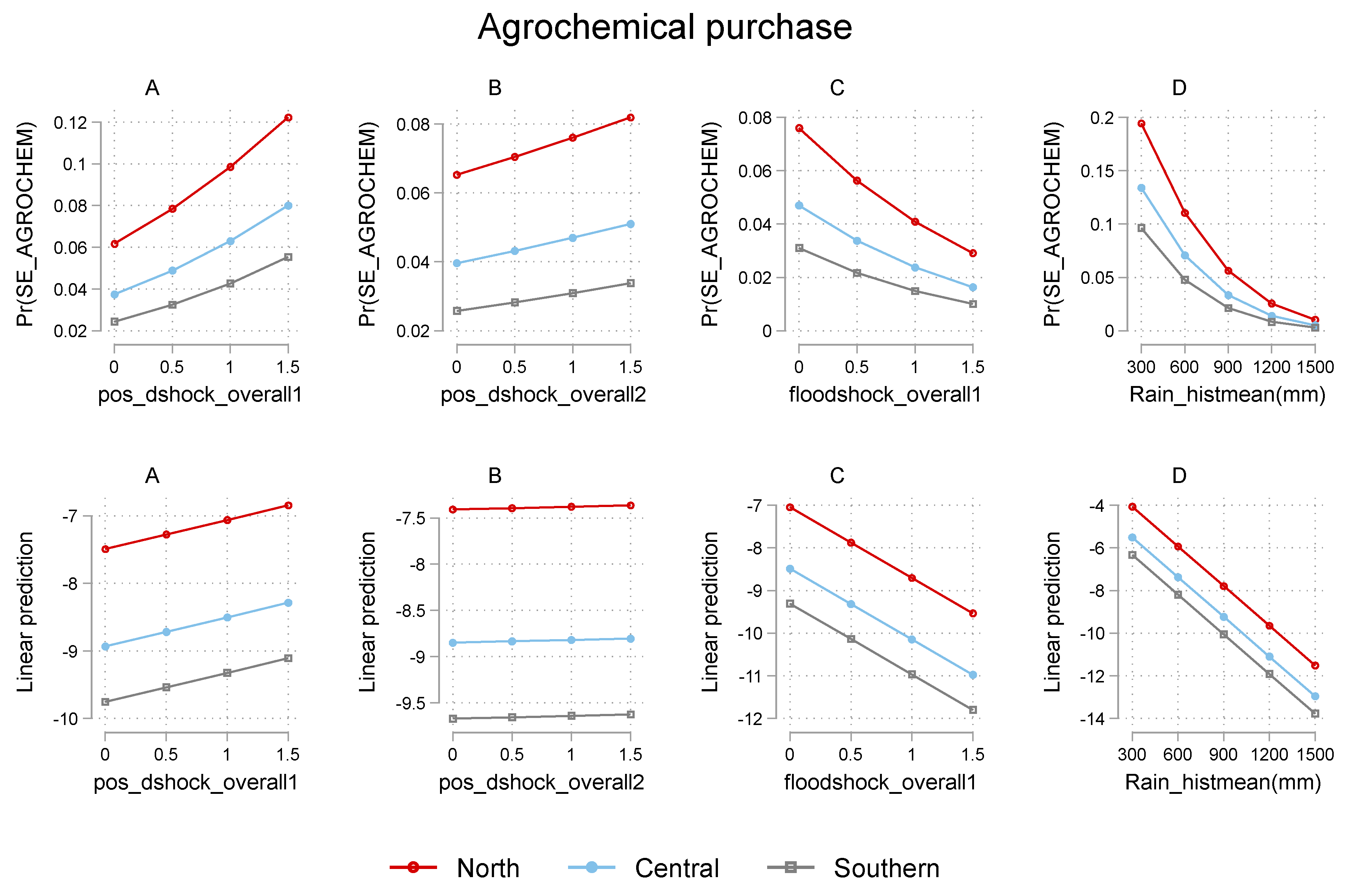
In Table 4, we report results from the model of agrochemical input purchasing. We learn from the findings that a 1-year lag of drought shock enhances the likelihood of purchasing agrochemicals in the national sample and all three regions studied. Additionally, the 2-year lag of drought shock exposure enhances the probability of purchasing agrochemicals in the national sample and the southern region (Table 4).

Regarding flood shocks, results show that a recent exposure to a flood shock (1-year lag flood shock) reduces the likelihood of purchasing agrochemicals in the national sample, particularly in the southern region (Table 4). The long-term average rainfall is also associated with an increased likelihood of purchasing agrochemicals in the national sample, particularly in central and southern regions. Additionally, long-term average temperatures increase the chances of agrochemical purchase in the national sample, northern, and southern regions (Table 4).

Table 4. The influence of rainfall shocks on agrochemical purchase across regions in Malawi.

	National		Northern		Central		Southern
VARIABLES	Hurdle1	Hurdle2	Hurdle1	Hurdle2	Hurdle1	Hurdle2	Hurdle1	Hurdle2
Climate risk variables
Growing season drought shock (1-year lag)	0.039 *** (0.0084)	0.115 (0.1274)	0.045 *** (0.0145)	0.254 (0.2301)	0.024 * (0.0141)	−0.549 (0.5205)	0.069 *** (0.0220)	−0.154 (0.2598)
Growing season drought shock (2-year lag)	0.011 * (0.0067)	−0.087 (0.1194)	0.010 (0.0211)	0.068 (0.4118)	0.000 (0.0333)	−0.950 (0.7597)	0.050 *** (0.0148)	−0.460 * (0.2549)
Growing season flood shock (1-year lag)	−0.022 ** (0.0086)	−0.049 (0.1349)	−0.012 (0.0165)	0.149 (0.1864)	0.007 (0.0176)	0.198 (0.4681)	−0.044 ** (0.0175)	0.020 (0.2488)
Long-term season average rainfall (mm)	0.000 ** (0.0000)	0.001 (0.0008)	0.000 (0.0001)	−0.000 (0.0009)	−0.000 (0.0001)	0.004 * (0.0022)	0.000 *** (0.0001)	−0.001 (0.0016)
Long-term season average temperature (deg)	0.005 *** (0.0018)	−0.020 (0.0266)	0.011 ** (0.0046)	0.049 (0.0542)	−0.000 (0.0030)	−0.068 (0.0468)	0.008 *** (0.0026)	−0.023 (0.0408)
Other control variables	Yes	Yes	Yes	Yes	Yes	Yes	Yes	Yes
Sigma constant		0.698 *** (0.0168)		0.633 *** (0.0356)		0.747 *** (0.0323)		0.654 *** (0.0215)
Survey year dummies	Yes	Yes	Yes	Yes	Yes	Yes	Yes	Yes
District fixed effects	Yes	Yes	Yes	Yes	Yes	Yes	Yes	Yes
Observations	25,631	906	4123	138	9001	290	12,502	478

Notes: Cluster robust standard errors are in parenthesis. Hurdle 1 is a probit regression for the probability of using purchased agrochemicals while Hurdle 2 is the model for intensity of agrochemical purchase for purchasers (log value of purchased agrochemicals (USD/ha), * p < 0.10, ** p < 0.05, *** p < 0.01.

Table 4. The influence of rainfall shocks on agrochemical purchase across regions in Malawi.

	National		Northern		Central		Southern
VARIABLES	Hurdle1	Hurdle2	Hurdle1	Hurdle2	Hurdle1	Hurdle2	Hurdle1	Hurdle2
Climate risk variables
Growing season drought shock (1-year lag)	0.039 *** (0.0084)	0.115 (0.1274)	0.045 *** (0.0145)	0.254 (0.2301)	0.024 * (0.0141)	−0.549 (0.5205)	0.069 *** (0.0220)	−0.154 (0.2598)
Growing season drought shock (2-year lag)	0.011 * (0.0067)	−0.087 (0.1194)	0.010 (0.0211)	0.068 (0.4118)	0.000 (0.0333)	−0.950 (0.7597)	0.050 *** (0.0148)	−0.460 * (0.2549)
Growing season flood shock (1-year lag)	−0.022 ** (0.0086)	−0.049 (0.1349)	−0.012 (0.0165)	0.149 (0.1864)	0.007 (0.0176)	0.198 (0.4681)	−0.044 ** (0.0175)	0.020 (0.2488)
Long-term season average rainfall (mm)	0.000 ** (0.0000)	0.001 (0.0008)	0.000 (0.0001)	−0.000 (0.0009)	−0.000 (0.0001)	0.004 * (0.0022)	0.000 *** (0.0001)	−0.001 (0.0016)
Long-term season average temperature (deg)	0.005 *** (0.0018)	−0.020 (0.0266)	0.011 ** (0.0046)	0.049 (0.0542)	−0.000 (0.0030)	−0.068 (0.0468)	0.008 *** (0.0026)	−0.023 (0.0408)
Other control variables	Yes	Yes	Yes	Yes	Yes	Yes	Yes	Yes
Sigma constant		0.698 *** (0.0168)		0.633 *** (0.0356)		0.747 *** (0.0323)		0.654 *** (0.0215)
Survey year dummies	Yes	Yes	Yes	Yes	Yes	Yes	Yes	Yes
District fixed effects	Yes	Yes	Yes	Yes	Yes	Yes	Yes	Yes
Observations	25,631	906	4123	138	9001	290	12,502	478

Notes: Cluster robust standard errors are in parenthesis. Hurdle 1 is a probit regression for the probability of using purchased agrochemicals while Hurdle 2 is the model for intensity of agrochemical purchase for purchasers (log value of purchased agrochemicals (USD/ha), * p < 0.10, ** p < 0.05, *** p < 0.01.

Figure 8. Plotting marginal effects of changes in 1-year lag drought shocks (pos_dshock_overall1), 2-year lag drought shock (pos_dshock_overall2), 1-year lag flood shock (floodshock_overall1), and historical mean rainfall (Rain_histmean (mm)) on the probability (top panel), and intensity of agrochemical purchase (bottom panel) by region.

Figure 8. Plotting marginal effects of changes in 1-year lag drought shocks (pos_dshock_overall1), 2-year lag drought shock (pos_dshock_overall2), 1-year lag flood shock (floodshock_overall1), and historical mean rainfall (Rain_histmean (mm)) on the probability (top panel), and intensity of agrochemical purchase (bottom panel) by region.

5.2.4. Seed

The results from the models of seed purchase are reported in Table 5, where we learn that the likelihood of purchasing seeds increases with prior exposure to drought shocks. Precisely, a 1-year lag of drought shock exposure increases the possibility of buying seeds in the national sample, northern region, and the intensity of seed purchase in the southern region. However, in the central region, a 1-year lag of drought shock reduces the intensity of seed purchase for purchasers. The 2-year lag drought shock increases the probability of seed purchase in the national sample and increases the likelihood and intensity of seed purchase in the northern and southern regions (Table 5). Overall results consistently confirm that past exposure to drought shocks enhance seed purchasing in the following seasons.

In addition, we also learn that a flood shock (1-year lag) reduces the likelihood of purchasing seeds in the national sample, central, and southern regions and enhances the intensity of seed purchasing in the northern region (Table 5). Long-term season average rainfall enhances the intensity of seed purchase in the national sample and the central region and both the likelihood and intensity of seed purchase in the southern region (Table 5). Long-term temperature also significantly enhances seed purchasing decisions in the southern region.

Table 5. The influence of rainfall shocks on seed purchasing across regions in Malawi.

	National		Northern		Central		Southern
VARIABLES	Hurdle1	Hurdle2	Hurdle1	Hurdle2	Hurdle1	Hurdle2	Hurdle1	Hurdle2
Climate risk variables
Growing season drought shock (1-year lag)	0.069 *** (0.0200)	−0.025 (0.0475)	0.080 ** (0.0372)	0.065 (0.0854)	0.012 (0.0378)	−0.370 *** (0.0922)	0.030 (0.0560)	0.377 *** (0.1225)
Growing season drought shock (2-year lag)	0.089 *** (0.0197)	0.031 (0.0432)	0.090 * (0.0536)	0.257 * (0.1339)	0.092 (0.0805)	−0.184 (0.1893)	0.141 *** (0.0425)	0.185 ** (0.0903)
Growing season flood shock (1-year lag)	−0.102 *** (0.0184)	0.080 (0.0520)	0.017 (0.0377)	0.255 ** (0.1087)	−0.066 * (0.0383)	−0.010 (0.1005)	−0.246 *** (0.0377)	−0.001 (0.1127)
Long-term season average rainfall (mm)	0.000 (0.0001)	0.001 *** (0.0003)	−0.000 (0.0002)	0.000 (0.0005)	0.000 (0.0002)	0.002 ** (0.0006)	0.001 ** (0.0002)	0.001 *** (0.0005)
Long-term season average temperature (deg)	0.003 (0.0039)	0.012 (0.0088)	−0.003 (0.0111)	0.006 (0.0243)	−0.006 (0.0060)	−0.022 (0.0156)	0.012 ** (0.0052)	0.031 *** (0.0114)
Other control variables	Yes	Yes	Yes	Yes	Yes	Yes	Yes	Yes
Sigma constant		0.831 *** (0.0083)		0.857 *** (0.0255)		0.861 *** (0.0160)		0.801 *** (0.0101)
Survey year dummies	Yes	Yes	Yes	Yes	Yes	Yes	Yes	Yes
District fixed effects	Yes	Yes	Yes	Yes	Yes	Yes	Yes	Yes
Observations	25,631	11,171	4123	1309	9001	3680	12,507	6182

Notes: Cluster robust standard errors are in parenthesis. Hurdle 1 is a probit regression for the probability of using purchased agrochemicals while Hurdle 2 is the model for intensity of purchased seeds for purchasers (log quantity of purchased seed (kg/ha), * p < 0.10, ** p < 0.05, *** p < 0.01.

Table 5. The influence of rainfall shocks on seed purchasing across regions in Malawi.

	National		Northern		Central		Southern
VARIABLES	Hurdle1	Hurdle2	Hurdle1	Hurdle2	Hurdle1	Hurdle2	Hurdle1	Hurdle2
Climate risk variables
Growing season drought shock (1-year lag)	0.069 *** (0.0200)	−0.025 (0.0475)	0.080 ** (0.0372)	0.065 (0.0854)	0.012 (0.0378)	−0.370 *** (0.0922)	0.030 (0.0560)	0.377 *** (0.1225)
Growing season drought shock (2-year lag)	0.089 *** (0.0197)	0.031 (0.0432)	0.090 * (0.0536)	0.257 * (0.1339)	0.092 (0.0805)	−0.184 (0.1893)	0.141 *** (0.0425)	0.185 ** (0.0903)
Growing season flood shock (1-year lag)	−0.102 *** (0.0184)	0.080 (0.0520)	0.017 (0.0377)	0.255 ** (0.1087)	−0.066 * (0.0383)	−0.010 (0.1005)	−0.246 *** (0.0377)	−0.001 (0.1127)
Long-term season average rainfall (mm)	0.000 (0.0001)	0.001 *** (0.0003)	−0.000 (0.0002)	0.000 (0.0005)	0.000 (0.0002)	0.002 ** (0.0006)	0.001 ** (0.0002)	0.001 *** (0.0005)
Long-term season average temperature (deg)	0.003 (0.0039)	0.012 (0.0088)	−0.003 (0.0111)	0.006 (0.0243)	−0.006 (0.0060)	−0.022 (0.0156)	0.012 ** (0.0052)	0.031 *** (0.0114)
Other control variables	Yes	Yes	Yes	Yes	Yes	Yes	Yes	Yes
Sigma constant		0.831 *** (0.0083)		0.857 *** (0.0255)		0.861 *** (0.0160)		0.801 *** (0.0101)
Survey year dummies	Yes	Yes	Yes	Yes	Yes	Yes	Yes	Yes
District fixed effects	Yes	Yes	Yes	Yes	Yes	Yes	Yes	Yes
Observations	25,631	11,171	4123	1309	9001	3680	12,507	6182

Notes: Cluster robust standard errors are in parenthesis. Hurdle 1 is a probit regression for the probability of using purchased agrochemicals while Hurdle 2 is the model for intensity of purchased seeds for purchasers (log quantity of purchased seed (kg/ha), * p < 0.10, ** p < 0.05, *** p < 0.01.

Figure 9. Plotting marginal effects of changes in 1-year lag drought shocks (pos_dshock_overall1), 2-year lag drought shock (pos_dshock_overall2), 1-year lag flood shock (floodshock_overall1), and historical mean rainfall (Rain_histmean (mm)) on the probability (top panel) and intensity of seed purchase (bottom panel) by region.

Figure 9. Plotting marginal effects of changes in 1-year lag drought shocks (pos_dshock_overall1), 2-year lag drought shock (pos_dshock_overall2), 1-year lag flood shock (floodshock_overall1), and historical mean rainfall (Rain_histmean (mm)) on the probability (top panel) and intensity of seed purchase (bottom panel) by region.

5.2.5. Hired Labor

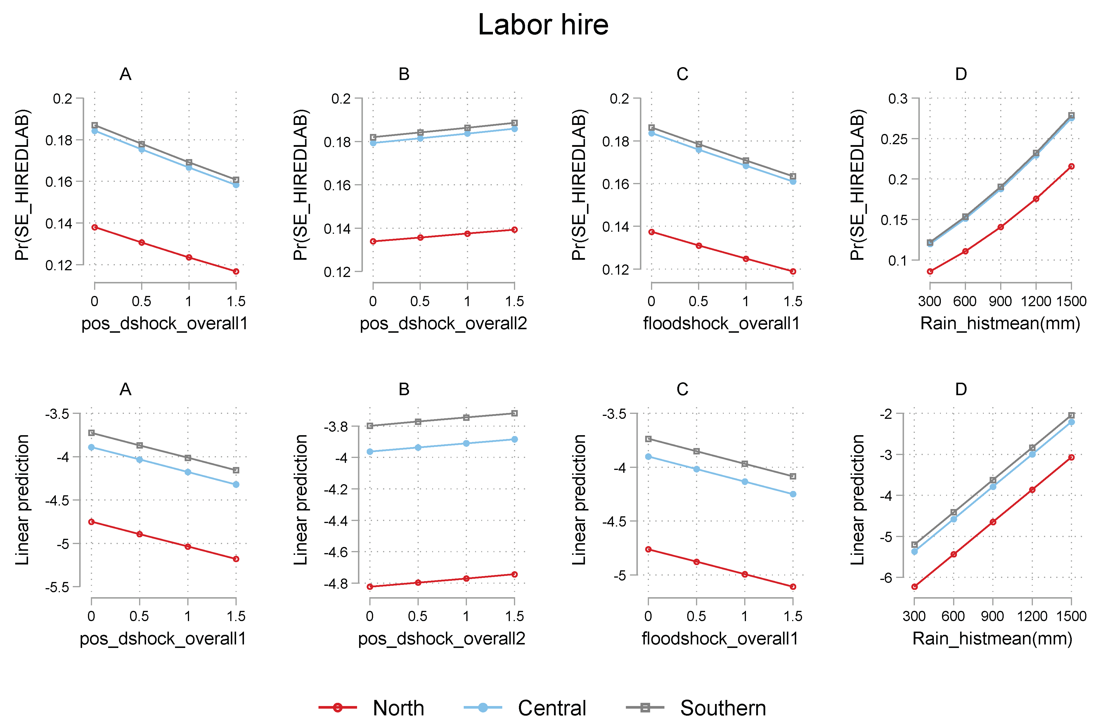
We present the results from the model of hired labor in Table 6. Results show that exposure to a 2-year lag of drought shock enhances the likelihood of hiring labor in the national sample and reduces the intensity of labor hiring for hirers in the southern region (Table 6). In addition, a 1-year lag flood shock enhances the intensity of labor hire in the northern region while reducing the chances of labor hire in the central region.

We also learn that long-term rainfall enhances the use and intensity of hired labor use in the national sample and the chances and intensity of hired labor use in the central and southern regions. More so, the long-term average temperature reduces the likelihood and intensity of hired labor use in the national sample, the intensity of hired labor use in the central region, and the likelihood of using hired labor in the southern region. Additionally, long-term temperature enhances the intensity of hired labor use in the northern region.

Table 6. The influence of rainfall shocks on hiring labor across regions in Malawi.

	National		Northern		Central		Southern
VARIABLES	Hurdle1	Hurdle2	Hurdle1	Hurdle2	Hurdle1	Hurdle2	Hurdle1	Hurdle2
Climate risk variables
Growing season drought shock (1-year lag)	−0.007 (0.0145)	−0.063 (0.0791)	0.042 (0.0281)	0.183 (0.1349)	−0.039 (0.0284)	−0.112 (0.1557)	−0.019 (0.0413)	0.095 (0.2328)
Growing season drought shock (2-year lag)	0.031 ** (0.0140)	−0.105 (0.0750)	0.063 (0.0401)	−0.358 (0.2266)	−0.013 (0.0630)	0.289 (0.3195)	0.004 (0.0294)	−0.522 *** (0.1608)
Growing season flood shock (1-year lag)	−0.018 (0.0149)	0.145 * (0.0758)	−0.037 (0.0266)	0.109 (0.1687)	−0.109 *** (0.0286)	0.041 (0.1615)	−0.018 (0.0325)	0.190 (0.1600)
Long-term season average rainfall (mm)	0.000 *** (0.0001)	0.001 * (0.0004)	0.000 (0.0001)	0.000 (0.0005)	0.000 ** (0.0002)	0.000 (0.0011)	0.000 (0.0002)	0.002 * (0.0008)
Long-term season average temperature (deg)	−0.008 ** (0.0031)	−0.027 * (0.0158)	−0.004 (0.0084)	0.065 * (0.0367)	−0.002 (0.0053)	−0.051 * (0.0287)	−0.014 *** (0.0041)	−0.028 (0.0197)
Other control variables	Yes	Yes	Yes	Yes	Yes	Yes	Yes	Yes
Sigma constant		0.899 *** (0.0096)		0.883 *** (0.0248)		0.901 *** (0.0169)		0.872 *** (0.0127)
Survey year dummies	Yes	Yes	Yes	Yes	Yes	Yes	Yes	Yes
District fixed effects	Yes	Yes	Yes	Yes	Yes	Yes	Yes	Yes
Observations	25,631	4433	4123	706	9001	1678	12,502	2049

Notes: Cluster robust standard errors in parenthesis. Hurdle 1 is a probit regression for the probability of using hired labor, while Hurdle 2 is the model for intensity of use (log days of hired labor (#/ha), * p < 0.10, ** p < 0.05, *** p < 0.01.

Table 6. The influence of rainfall shocks on hiring labor across regions in Malawi.

	National		Northern		Central		Southern
VARIABLES	Hurdle1	Hurdle2	Hurdle1	Hurdle2	Hurdle1	Hurdle2	Hurdle1	Hurdle2
Climate risk variables
Growing season drought shock (1-year lag)	−0.007 (0.0145)	−0.063 (0.0791)	0.042 (0.0281)	0.183 (0.1349)	−0.039 (0.0284)	−0.112 (0.1557)	−0.019 (0.0413)	0.095 (0.2328)
Growing season drought shock (2-year lag)	0.031 ** (0.0140)	−0.105 (0.0750)	0.063 (0.0401)	−0.358 (0.2266)	−0.013 (0.0630)	0.289 (0.3195)	0.004 (0.0294)	−0.522 *** (0.1608)
Growing season flood shock (1-year lag)	−0.018 (0.0149)	0.145 * (0.0758)	−0.037 (0.0266)	0.109 (0.1687)	−0.109 *** (0.0286)	0.041 (0.1615)	−0.018 (0.0325)	0.190 (0.1600)
Long-term season average rainfall (mm)	0.000 *** (0.0001)	0.001 * (0.0004)	0.000 (0.0001)	0.000 (0.0005)	0.000 ** (0.0002)	0.000 (0.0011)	0.000 (0.0002)	0.002 * (0.0008)
Long-term season average temperature (deg)	−0.008 ** (0.0031)	−0.027 * (0.0158)	−0.004 (0.0084)	0.065 * (0.0367)	−0.002 (0.0053)	−0.051 * (0.0287)	−0.014 *** (0.0041)	−0.028 (0.0197)
Other control variables	Yes	Yes	Yes	Yes	Yes	Yes	Yes	Yes
Sigma constant		0.899 *** (0.0096)		0.883 *** (0.0248)		0.901 *** (0.0169)		0.872 *** (0.0127)
Survey year dummies	Yes	Yes	Yes	Yes	Yes	Yes	Yes	Yes
District fixed effects	Yes	Yes	Yes	Yes	Yes	Yes	Yes	Yes
Observations	25,631	4433	4123	706	9001	1678	12,502	2049

Notes: Cluster robust standard errors in parenthesis. Hurdle 1 is a probit regression for the probability of using hired labor, while Hurdle 2 is the model for intensity of use (log days of hired labor (#/ha), * p < 0.10, ** p < 0.05, *** p < 0.01.

Figure 10. Plotting marginal effects of changes in 1-year lag drought shocks (pos_dshock_overall1), 2-year lag drought shock (pos_dshock_overall2), 1-year lag flood shock (floodshock_overall1), and historical mean rainfall (Rain_histmean (mm)) on the probability (top panel) and intensity of labor purchase (bottom panel) by region.

Figure 10. Plotting marginal effects of changes in 1-year lag drought shocks (pos_dshock_overall1), 2-year lag drought shock (pos_dshock_overall2), 1-year lag flood shock (floodshock_overall1), and historical mean rainfall (Rain_histmean (mm)) on the probability (top panel) and intensity of labor purchase (bottom panel) by region.

5.3. Heterogeneities—Wealth, Gender, and Access to Information

Farming households usually choose climate change adaptation strategies such as input purchasing mainly as a function of resource endowments (land, household assets, and labor) at their disposal [48,49]. Having gathered evidence that recent past exposure to drought shocks largely encourages input purchasing across regions in Malawi, we further explore the impact of drought shocks in relatively richer and poorer households and male- vs. female-headed households. The intention is to test whether the impact of drought shocks is the same for households in different strata of socioeconomic status (wealth and gender) and access to information regarding input purchasing. We present summarized results in

Table 7. The influence of rainfall shocks on input purchasing by wealth endowments.

	All Inputs		Fertilizer		Agrochemicals		Seed		Hired labor
	Hurdle1	Hurdle2	Hurdle1	Hurdle2	Hurdle1	Hurdle2	Hurdle1	Hurdle2	Hurdle1	Hurdle2
High asset endowments
Growing season drought shock (1-year lag)	0.093 *** (0.0253)	0.143 ** (0.0729)	0.065 *** (0.0243)	0.123 ** (0.0541)	0.065 *** (0.0124)	0.121 (0.1360)	0.099 *** (0.0238)	−0.021 (0.0580)	−0.004 (0.0209)	−0.079 (0.0920)
Growing season drought shock (2-year lag)	0.110 *** (0.0249)	0.074 (0.0748)	0.092 *** (0.0244)	0.129 ** (0.0590)	0.022 ** (0.0107)	−0.030 (0.1422)	0.114 *** (0.0228)	−0.016 (0.0546)	0.027 (0.0205)	−0.125 (0.0843)
Growing season flood shock (1-year lag)	−0.118 *** (0.0298)	0.281 *** (0.0739)	0.043 * (0.0222)	0.046 (0.0573)	−0.029 ** (0.0140)	−0.117 (0.1474)	−0.092 *** (0.0230)	0.092 (0.0682)	−0.004 (0.0227)	0.104 (0.0849)
Long-term season average rainfall (mm)	0.000 (0.0002)	0.002 *** (0.0005)	0.000 (0.0002)	0.002 *** (0.0004)	0.000 ** (0.0001)	0.000 (0.0009)	0.000 (0.0001)	0.001 ** (0.0004)	0.000 ** (0.0001)	0.001 (0.0005)
Long-term season average temperature (deg)	−0.018 *** (0.0064)	−0.183 *** (0.0154)	−0.058 *** (0.0053)	−0.078 *** (0.0114)	0.007 *** (0.0026)	−0.021 (0.0292)	0.002 (0.0048)	0.011 (0.0117)	−0.009 ** (0.0047)	−0.032 * (0.0182)
Other control variables	Yes	Yes	Yes	Yes	Yes	Yes	Yes	Yes	Yes	Yes
Survey year dummies	Yes	Yes	Yes	Yes	Yes	Yes	Yes	Yes	Yes	Yes
District fixed effects	Yes	Yes	Yes	Yes	Yes	Yes	Yes	Yes	Yes	Yes
Observations	12,815	8334	12,815	5628	12,789	695	12,815	5972	12,815	3217
Low asset endowments
Growing season drought shock (1-year lag)	0.010 (0.0273)	0.022 (0.0981)	−0.017 (0.0231)	−0.015 (0.0918)	0.010 (0.0089)	−0.249 (0.2809)	0.023 (0.0269)	−0.050 (0.0755)	−0.004 (0.0158)	−0.006 (0.1255)
Growing season drought shock (2-year lag)	0.073 *** (0.0258)	−0.104 (0.0844)	0.018 (0.0228)	−0.099 (0.0905)	−0.004 (0.0059)	0.020 (0.2918)	0.051 ** (0.0260)	0.095 (0.0618)	0.035 ** (0.0147)	−0.078 (0.1399)
Growing season flood shock (1-year lag)	−0.189 *** (0.0284)	0.263 *** (0.0865)	−0.003 (0.0206)	0.099 (0.0854)	−0.016 ** (0.0073)	0.393 (0.2861)	−0.111 *** (0.0233)	0.050 (0.0661)	−0.032 ** (0.0137)	0.252 * (0.1387)
Long-term season average rainfall (mm)	0.000 ** (0.0002)	0.001 ** (0.0005)	0.000 (0.0001)	0.001 ** (0.0005)	0.000 (0.0000)	0.000 (0.0021)	0.000 (0.0001)	0.001 *** (0.0004)	0.000 * (0.0001)	0.001 (0.0008)
Long-term season average temperature (deg)	−0.010 * (0.0053)	−0.166*** (0.0168)	−0.043 *** (0.0045)	−0.111 *** (0.0154)	0.003 * (0.0016)	−0.052 (0.0518)	0.003 (0.0049)	0.012 (0.0111)	−0.005 ** (0.0027)	−0.009 (0.0247)
Other control variables	Yes	Yes	Yes	Yes	Yes	Yes	Yes	Yes	Yes	Yes
Survey year dummies	Yes	Yes	Yes	Yes	Yes	Yes	Yes	Yes	Yes	Yes
District fixed effects	Yes	Yes	Yes	Yes	Yes	Yes	Yes	Yes	Yes	Yes
Observation	12,816	6724	12,816	3168	12,075	211	12,816	5199	12,796	1216

Notes: Cluster robust standard errors are in parenthesis. Hurdle 1 is a probit regression for the probability of input purchase while Hurdle 2 is the model for intensity of purchase for purchasers, * p < 0.10, ** p < 0.05, *** p < 0.01.

,

Table 8. The influence of rainfall shocks on input purchasing by gender of household head.

	All Inputs		Fertilizer		Agrochemicals		Seed		Hired Labor
	Hurdle1	Hurdle2	Hurdle1	Hurdle2	Hurdle1	Hurdle2	Hurdle1	Hurdle2	Hurdle1	Hurdle2
Female-Headed
Growing season drought shock (1-year lag)	0.030 (0.0309)	0.017 (0.1108)	−0.030 (0.0262)	0.043 (0.1007)	0.005 (0.0072)	−0.063 (0.3538)	0.020 (0.0315)	−0.053 (0.0782)	0.006 (0.0205)	0.158 (0.1404)
Growing season drought shock (2-year lag)	0.137 *** (0.0279)	−0.066 (0.0995)	0.045 * (0.0231)	0.079 (0.1073)	0.009 (0.0070)	0.275 (0.2801)	0.147 *** (0.0284)	−0.042 (0.0760)	0.009 (0.0177)	0.009 (0.1340)
Growing season flood shock (1-year lag)	−0.153 *** (0.0319)	0.236 ** (0.1189)	−0.006 (0.0240)	0.082 (0.1169)	−0.027 ** (0.0133)	−0.815 * (0.4882)	−0.127 *** (0.0313)	0.052 (0.0996)	−0.005 (0.0207)	0.329 ** (0.1525)
Long-term season average rainfall (mm)	−0.000 (0.0001)	0.001 (0.0005)	−0.000 (0.0001)	0.000 (0.0005)	−0.000** (0.0000)	0.002 * (0.0010)	−0.000 (0.0001)	0.000 (0.0004)	0.000 *** (0.0001)	0.000 (0.0005)
Long-term season average temperature (deg)	−0.015 *** (0.0041)	−0.187 *** (0.0144)	−0.050 *** (0.0033)	−0.111 *** (0.0146)	0.006 *** (0.0013)	0.085 *** (0.0328)	0.007 * (0.0040)	0.015 (0.0098)	−0.005 ** (0.0028)	−0.020 (0.0177)
Other control variables	Yes	Yes	Yes	Yes	Yes	Yes	Yes	Yes	Yes	Yes
Survey year dummies	Yes	Yes	Yes	Yes	Yes	Yes	Yes	Yes	Yes	Yes
District fixed effects	Yes	Yes	Yes	Yes	Yes	Yes	Yes	Yes	Yes	Yes
Observations	7432	3820	7432	1863	7432	146	7432	2879	7432	1096
Male-headed
Growing season drought shock (1-year lag)	0.049 ** (0.0225)	0.185 *** (0.0652)	0.051** (0.0230)	0.101 ** (0.0504)	0.022 ** (0.0090)	0.005 (0.1281)	0.036 * (0.0220)	−0.009 (0.0494)	−0.014 (0.0167)	−0.121 (0.0934)
Growing season drought shock (2-year lag)	0.092 *** (0.0234)	0.023 (0.0659)	0.037* (0.0220)	0.064 (0.0587)	0.011 (0.0082)	−0.142 (0.1133)	0.108 *** (0.0212)	0.116 ** (0.0454)	0.036 ** (0.0159)	−0.238 *** (0.0836)
Growing season flood shock (1-year lag)	−0.173 *** (0.0280)	0.280 *** (0.0687)	0.033 (0.0205)	0.017 (0.0567)	−0.031 *** (0.0121)	−0.040 (0.1416)	−0.132 *** (0.0207)	0.049 (0.0574)	−0.037 ** (0.0169)	0.045 (0.0850)
Long-term season average rainfall (mm)	−0.000 (0.0001)	0.001 *** (0.0003)	0.000 (0.0001)	0.001 *** (0.0002)	−0.000 (0.0000)	0.001 ** (0.0005)	−0.000 (0.0001)	0.001 *** (0.0002)	0.000 *** (0.0001)	0.001 *** (0.0004)
Long-term season average temperature (deg)	−0.015 *** (0.0035)	−0.179 *** (0.0090)	−0.063 *** (0.0029)	−0.091 *** (0.0076)	0.013 *** (0.0014)	0.033 * (0.0185)	0.007 ** (0.0028)	0.016 *** (0.0063)	−0.002 (0.0023)	−0.045 *** (0.0110)
Other control variables	Yes	Yes	Yes	Yes	Yes	Yes	Yes	Yes	Yes	Yes
Survey year dummies	Yes	Yes	Yes	Yes	Yes	Yes	Yes	Yes	Yes	Yes
District fixed effects	Yes	Yes	Yes	Yes	Yes	Yes	Yes	Yes	Yes	Yes
Observation	18,199	11,238	18,199	6933	18,199	760	18,199	8292	18,199	3337

Notes: Cluster robust standard errors are in parenthesis. Hurdle 1 is a probit regression for the probability of input purchase while Hurdle 2 is the model for intensity of purchase for purchasers, * p < 0.10, ** p < 0.05, *** p < 0.01.

and

Table 9. The influence of rainfall shocks on input purchasing by access to information.

	All Inputs		Fertilizer		Agrochemicals		Seed		Hired Labor
	Hurdle1	Hurdle2	Hurdle1	Hurdle2	Hurdle1	Hurdle2	Hurdle1	Hurdle2	Hurdle1	Hurdle2
Access to information
Growing season drought shock (1-year lag)	0.072 *** (0.0205)	0.274 *** (0.0664)	0.071 *** (0.0219)	0.176 *** (0.0514)	0.024 *** (0.0086)	0.079 (0.1251)	0.042 * (0.0218)	−0.018 (0.0488)	−0.004 (0.0161)	0.033 (0.0898)
Growing season drought shock (2-year lag)	0.136 *** (0.0231)	0.018 (0.0684)	0.076 *** (0.0226)	0.021 (0.0662)	0.010 (0.0084)	−0.149 (0.1190)	0.145 *** (0.0232)	0.052 (0.0501)	0.029 * (0.0161)	−0.087 (0.0869)
Growing season flood shock (1-year lag)	−0.106 *** (0.0305)	0.299 *** (0.0821)	0.052 ** (0.0241)	0.023 (0.0715)	−0.036 *** (0.0137)	0.006 (0.1722)	−0.126 *** (0.0266)	0.082 (0.0661)	−0.006 (0.0197)	0.162 * (0.0983)
Long-term season average rainfall (mm)	−0.000 (0.0001)	0.001 *** (0.0003)	0.000 (0.0001)	0.001 *** (0.0002)	−0.000 * (0.0000)	0.002 *** (0.0005)	−0.000 (0.0001)	0.001 *** (0.0002)	0.000 *** (0.0001)	0.001 ** (0.0004)
Long-term season average temperature (deg)	−0.014 *** (0.0033)	−0.169 *** (0.0096)	−0.057 *** (0.0030)	−0.093 *** (0.0084)	0.012 *** (0.0015)	0.060 *** (0.0189)	0.005 * (0.0030)	0.024 *** (0.0065)	−0.002 (0.0022)	−0.046 *** (0.0113)
Other control variables	Yes	Yes	Yes	Yes	Yes	Yes	Yes	Yes	Yes	Yes
Survey year dummies	Yes	Yes	Yes	Yes	Yes	Yes	Yes	Yes	Yes	Yes
District fixed effects	Yes	Yes	Yes	Yes	Yes	Yes	Yes	Yes	Yes	Yes
Observations	16152	10065	16152	6059	16152	670	16152	7468	16152	3033
No access to information
Growing season drought shock (1-year lag)	−0.022 (0.0368)	−0.164 (0.1174)	−0.068 ** (0.0303)	−0.113 (0.0953)	0.005 (0.0094)	−0.176 (0.2762)	0.003 (0.0363)	−0.018 (0.0906)	−0.022 (0.0246)	−0.257 * (0.1500)
Growing season drought shock (2-year lag)	0.059 * (0.0308)	−0.038 (0.0941)	−0.020 (0.0249)	0.136 (0.0836)	0.015 * (0.0079)	−0.067 (0.1936)	0.083 *** (0.0283)	0.102 (0.0685)	0.035 * (0.0199)	−0.366 *** (0.1242)
Growing season flood shock (1-year lag)	−0.239 *** (0.0304)	0.195 ** (0.0950)	−0.007 (0.0217)	−0.005 (0.0785)	−0.025 ** (0.0102)	−0.241 (0.1923)	−0.141 *** (0.0244)	−0.001 (0.0707)	−0.052 *** (0.0190)	0.037 (0.1323)
Long-term season average rainfall (mm)	0.000 (0.0001)	−0.000 (0.0004)	−0.000 * (0.0001)	0.000 (0.0004)	−0.000 (0.0000)	0.001 (0.0009)	−0.000 (0.0001)	0.001 ** (0.0003)	0.000 *** (0.0001)	0.001 (0.0005)
Long-term season average temperature (deg)	−0.016 *** (0.0046)	−0.210 *** (0.0133)	−0.064 *** (0.0034)	−0.104 *** (0.0123)	0.009 *** (0.0015)	−0.002 (0.0286)	0.009 ** (0.0037)	0.004 (0.0097)	−0.005 * (0.0031)	−0.028 (0.0173)
Other control variables	Yes	Yes	Yes	Yes	Yes	Yes	Yes	Yes	Yes	Yes
Survey year dummies	Yes	Yes	Yes	Yes	Yes	Yes	Yes	Yes	Yes	Yes
District fixed effects	Yes	Yes	Yes	Yes	Yes	Yes	Yes	Yes	Yes	Yes
Observations	9479	4993	9479	2737	9479	236	9479	3703	9479	1400

Notes: Cluster robust standard errors are in parenthesis. Hurdle 1 is a probit regression for the probability of input purchase while Hurdle 2 is the model for intensity of purchase for purchasers, * p < 0.10, ** p < 0.05, *** p < 0.01.

.

From the results, we see that drought shocks (1- and 2-year lags) significantly and to a greater extent enhance the probability and intensity of input purchasing in general, particularly for key inputs (fertilizer, seed, and agrochemicals) in the group of relatively richer households compared to their poorer counterparts (Table 7). The implication is that wealthier households are more likely to purchase inputs following exposure to drought shocks, unlike their poorer counterparts.

Comparing the results in male- and female-headed households provides additional insights. From the results, we see that drought shocks (1- and 2-year lags) significantly enhance the probability and intensity of input purchasing in general, particularly for key inputs (fertilizer, seed, and agrochemicals) in male-headed households compared to female-headed households (Table 8).

Furthermore, when we compare the impact of climate risk variables, particularly drought shocks, on decisions to invest in commercial inputs through purchase, we establish that, for farmers with access to agricultural information, lagged drought shocks largely enhance input purchase decisions (in general and for specific inputs, e.g., fertilizer, agrochemicals, seed, and labor) (Table 9). However, for those without access to information, the relationships are mostly insignificant and, in some cases, negative (e.g., 1-year lag drought shock on fertilizer purchase) compared to those with access to information (Table 9).

6. Discussion

We discuss our key findings on the influence of covariate rainfall shocks in stimulating commercial input purchasing in heterogeneous settings in Malawi and derive implications for input market developments that can support climate change adaptation in smallholder agriculture. From the study, we can reveal a few relevant findings for discussion: (i) First, we gather overwhelming evidence that recent past exposure to drought shocks has largely encouraged input purchasing across regions in general, particularly for agrochemicals, fertilizer, seed, and labor. Drought and flood shocks are confirmed key determinants of commercial input purchasing by objective and subjective measures of rainfall shocks. Input purchase decisions appear more responsive to climate risk variables in the drier southern and central regions than in the northern region. However, in some instances, we have established that drought shocks, although they enhance the likelihood of input purchasing, also reduce purchase intensity. For instance, we established that drought shocks reduce the intensity of input purchasing in the northern region and the intensity of labor hiring in the southern region. (ii) Second, we also establish that drought and flood shocks do not necessarily prompt similar responses in input purchasing decisions by farmers. We learn that flood shocks reduce the likelihood of purchasing some inputs, for example seeds, in all the regions but enhance the intensity of purchase in some regions, e.g., the northern region. (iii) Third, we have established that relatively richer households with access to information and male-headed households are more likely to purchase inputs following drought shock exposure when compared to their opposite counterparts.

6.1. Impact of Rainfall Shocks on Input Purchasing Decisions in Different Regions in Malawi

6.1.1. Inorganic Fertilizers

Based on the findings, particularly the national sample results, we could not reject our hypothesis that previous exposure to drought shocks enhance fertilizer purchasing in the following seasons in Malawi. Access to inorganic fertilizers through purchasing is beneficial in helping farmers adapt to climate change. Given the devastating effects of the continued exposure to drought shocks coupled with poor soil fertility on crop yields and food insecurity [63], farmers are willing to invest in inorganic fertilizers to stabilize and/or reduce the risk of total crop failure under rainfall stress. Our findings corroborate the available literature that has demonstrated that investment in integrated soil fertility management (ISFM) technologies protect against climate risk; in particular, previous exposure to dry spells influences the use of ISFM in Malawi [25]. Inorganic fertilizer purchasing becomes more important under a changing climate as it complements on-farm organic fertilizer sources such as manure that may become less reliable with increased climate variability (e.g., manure production could fall on the farm due to possible loss of livestock due to diseases and pests that may arise with extreme weather events). Furthermore, access to purchased inorganic fertilizers also allows farmers to implement climate-resilient micro-dosing fertilizer application techniques proven to offer sufficient nutrition in highly degraded soil in a sustainable fashion [41,42].

However, heterogeneity in the influence of drought shocks in studied regions and the effects of drought and flood shocks on fertilizers provide additional insights. Drought shocks were found to reduce the chances of fertilizer purchase in the northern region, while flood shocks enhanced the intensity of fertilizer purchasing. These contrasting findings could be linked to different climate and agro-ecological conditions in the northern compared to the central and southern regions and the heterogeneity in possible shock responses to innovative technology adoption. Farmers in the northern region generally experience comparably higher rainfall conditions and cooler temperatures (Figure 1 and Figure 4), which could explain the heterogeneities. Additionally, drought shocks can significantly reduce farmers’ purchasing power, limiting the chances of purchasing fertilizers after drought shock exposure. On the contrary, flood shocks experienced in prior seasons could stimulate the purchase of more inorganic fertilizers in the following seasons when flood shocks are anticipated due to the possibility of fertilizer leaching with excessive rain, a phenomenon common in regions that receive more rainfall, such as the case in the northern region.

6.1.2. Agrochemicals

Despite agrochemical input purchasing being a less common practice in the studied sample, we could not reject our hypothesis that past exposure to drought shocks in the national sample and all studied regions promotes agrochemical purchasing in the following seasons. Crop production, particularly maize production in Malawi, is highly susceptible to drought shocks and increased pest attacks. Therefore, farmers are willing to invest in modern crop protection methods to minimize yield losses from pest attacks. This notion is plausible given that climate variability and change have been associated with increased crop pests and diseases [36], which demand stern efforts in managing through agrochemical use. Using some examples from Malawi, we learn that, in some parts of the country, e.g., the Mwansambo area from the central region, rainfall variability in the form of dry spells has been associated with increased fall armyworm infestations in maize fields [37]. Thus, investment in agrochemical use may help farmers deal with increased pest attacks that are probable with amplified rainfall variability, hence offering adaptation to climate change.

On the contrary, positive rainfall deviations are found to reduce agrochemical purchasing. A possible explanation could be that past exposure to positive rainfall deviations probably did not bring severe problems with pest and disease attacks, causing them to be reluctant to invest in purchasing agrochemicals when they anticipate flood shocks in the future. However, given the limited rates of purchasing agrochemicals in the analyzed sample, future research is needed to explore this aspect further.

6.1.3. Seed

We could not reject our hypothesis that previous exposure to drought shocks encourages seed purchasing in the following seasons. The result could be explained by the fact that although farmers in developing regions, such as Malawi, often rely on farmer-saved seeds, exposure to drought shocks in prior seasons increase the demand for purchased seeds [12,64]. This notion is also supported by the fact that using on-farm seed sources alone with an increased climate risk may render crop yields more vulnerable [38], which calls for the diversification of farmer-saved seeds with seeds sourced from other channels. For instance, in Malawi, drought-tolerant maize varieties have been proven to enhance the resilience of maize yields to climate stress [39,40]. The implication is that access to purchased seeds may allow smallholder farmers to diversify their conventional seed varieties with other resilient varieties available on the market.

In addition, flood shocks were found to reduce the likelihood of purchasing seed in the national sample, particularly the central and southern regions, but also enhance the intensity of purchase in the northern region. The results could largely be explained by the fact that positive rainfall deviations (flood shocks) may lead to more possibilities than constraints regarding seed production and saving seeds from harvest for use in the following seasons. Positive rainfall deviations in the recent past may support the possibility of producing enough seeds by farmers, which are saved for use in the following seasons. The contrasting result of flood shocks in the northern region could be explained by the fact that anticipated favorable rainfall deviations (flood shocks) encourage intensified crop production in the same way as drought shocks.

6.1.4. Hired Labor

On the one hand, drought shocks enhance labor hiring in the national sample and the intensity of labor hiring in the southern region. On the other hand, flood shocks enhance the intensity of labor hire in the northern region while reducing the chances of labor hire in the central region. We failed to reject our hypothesis based on the national sample that previous drought shock exposure enhances the demand for hired labor in the following seasons. This notion could be explained by the idea that adapting to climate change may require supplementing family labor with off-farm labor. Supplementing family labor can be beneficial when the household faces labor shortages in general or when new skills are required to effectively implement innovations or technologies relevant for climate change adaptation. For instance, climate-smart practices such as (manual) conservation agriculture (CA) practices (implementing conservation agricultural practices on larger farms, which often includes the digging of planting basins and manual weeding using hand hoes that require more labor than conventional plough-based farming) were previously reported to increase labor demand at the household level [43,65], thus increasing the need to hire laborers off-farm. However, due to the possible effects of drought shocks on reducing purchasing power by households, it is also possible that drought shocks can lessen the intensity of labor hiring, as we found in the southern region. Additionally, the result from the northern region that portrays positive rainfall deviations (flood shocks) to stimulate the enhanced intensity of labor hiring could imply that in the northern region, positive rainfall deviations create possibilities rather than limitations for enhanced labor hiring in coming seasons, as found with other inputs (e.g., seed, fertilizer).

6.2. Asset Wealth, Gender, and Information Access Heterogeneities

The result indicating that richer households are more likely to purchase inputs and to a greater extent following drought shock exposure than their poorer counterparts reveal that poorer households are more vulnerable to drought shocks. This finding aligns with the literature that considers household wealth endowments as an essential cushion for rural households against shocks [48,49,66,67]. Households better endowed with assets are more resilient to shocks and have higher chances of buying inputs post-shock exposure to help them deal with shocks in the coming seasons. Additionally, female-headed households, especially those in single relationships with fewer assets, are more vulnerable to shocks as they are less likely to purchase inputs in response to rainfall shocks. The results here could confirm the existence of gender disparities in climate change vulnerability emanating from both endowment and structural factors [52,68]. Female-headed families in the sample have fewer assets (land and non-land assets), low access to information, and access to borrowed credit. These could be some mechanisms behind their impaired response to shocks compared to male-headed households. More research is needed to further investigate the mechanisms (and their interactions) through which the gender disparities in input purchasing as a response to climate shocks arise. Additionally, access to information reduces transaction costs associated with the search, negotiation, and access to inputs from available markets [44,69,70], which explains why farmers with access to information were found to respond more positively to previous drought shock exposure compared to their counterparts.

7. Conclusions and Implications for Policy

From the results, we can conclude that input purchasing decisions are responsive to rainfall variability and recent shocks. This conclusion is true when objectively or subjectively measured rainfall shock variables are used. Having access to inputs through local markets helps smallholder farmers adjust their input mix to adapt and/or cope with climate risk. Access to inputs through purchase brings the necessary diversity in input options that the farmers need to adapt to shocks. Given the persistent exposure of farmers to rainfall shocks, particularly drought shocks in Malawi, leading to severe crop failure, mostly in drier central and southern regions [32], coupled with weak or missing agricultural insurance markets, our findings bear significant implications for climate resilience. Improving resilience to climate change in agriculture will require farmers to access risk-substituting inputs through purchase or other channels. Policy efforts should enhance or encourage active participation through public and private marketing institutions in local input distribution and marketing to improve the availability of diverse agricultural inputs that will eventually support the scaling success of climate adaptation efforts. Given that it is mainly the better-endowed, male-headed households, and those with access to information that have a higher propensity and tenacity to invest in purchased inputs, policy interventions aiming to enhance household resilience to climate shocks must be inclusive of the most vulnerable population (including poor and female-headed households) and enhance access to climate information services. Additionally, given the inter-regional variations in biophysical factors, socioeconomic development, and environmental conditions prompting different responses to shocks, policy efforts must consider having different development needs and priorities for specific regions.

Through its National Agricultural Policy (NAP) (GOM 2016a), the government of Malawi supports climate change adaptation in agriculture by promoting climate-smart agriculture (CSA). This is also evidenced in the recently launched National Agriculture Investment Plan (NAIP), which is now the main implementation vehicle for NAP, in which “resilient livelihoods and agricultural systems” is one of the four programs. Malawi’s National Agriculture Investment Plan (NAIP) has four programs: (1) policies, institutions, and coordination, (2) resilient livelihoods and agricultural systems, (3) production and productivity, and (4) markets, value addition, trade and finance, all targeted at transforming agriculture. Adaptation to shocks is evidently a key target for policy. Findings from this study support market development-related interventions that will enhance the supply of inputs in local markets (supply-side efforts). They deserve elevated attention and continuous updates in current CSA policies to help accelerate adaptation to climate change. In addition, demand-side efforts are needed to enhance both the physical and economic access to inputs for smallholder farmers through the market. For instance, scaling up quality extension services, access to credit, and other economic empowerment efforts that promote household asset build-up may help farmers use the market for adaptation effectively.

Given that Malawi has an already active agricultural input subsidy program assisting farmers in accessing inputs, it is imperative to mention that developing local input markets will complement such government efforts and help effect climate change adaptation.

Overall, the objective of promoting market growth is to ensure that farmers have access to a dynamic and diverse set of inputs that can provide them with the autonomy to respond to adverse climate change and enhance productivity and food security in a changing climatic environment. These recommendations primarily apply to Malawi but may also be relevant for neighboring countries facing similar conditions in persistent exposure to climate shocks with ravaging implications on agricultural productivity and food security.

References

- FAO. The State of the World’s Land and Water Resources for Food and Agriculture; FAO: Rome, Italy, 2013. [Google Scholar]
- Cooper, P.; Dimes, J.; Rao, K.; Shapiro, B.; Shiferaw, B.; Twomlow, S. Coping better with current climatic variability in the rain-fed farming systems of sub-Saharan Africa: An essential first step in adapting to future climate change? Agric. Ecosyst. Environ. 2008, 126, 24–35. [Google Scholar] [CrossRef] [Green Version]
- Devereux, S. The impact of droughts and floods on food security and policy options to alleviate negative effects. Agric. Econ. 2007, 37, 47–58. [Google Scholar] [CrossRef]
- Pauw, K.; Thurlow, J.; van Seventer, D. Droughts and Floods in Malawi. 2010. Available online: https://www.preventionweb.net/files/13792_ifpridp009621.pdf (accessed on 7 September 2022).
- Nangoma, E. National Adaptation Strategy to Climate Change Impacts: A Case Study of Malawi, 2008 (Human Development Report, 2007/2008); United Nations Development Program: New York, NY, USA, 2008. [Google Scholar]
- Giertz, A.; Caballero, J.; Galperin, D.; Makoka, D.; Olson, J.; German, G. Malawi Agricultural Sector Risk Assessment; World Bank: Washington, DC, USA, 2015. [Google Scholar]
- Clements, R.; Haggar, J.; Quezada, A.; Torres, J. Technologies for Climate Change Adaptation—Agriculture Sector.; UNEP: København, Denmark, 2011. [Google Scholar]
- Makate, C.; Makate, M.; Mango, N.; Siziba, S. Increasing resilience of smallholder farmers to climate change through multiple adoption of proven climate-smart agriculture innovations. Lessons from Southern Africa. J. Environ. Manag. 2019, 231, 858–868. [Google Scholar] [CrossRef]
- Pangapanga, P.I.; Jumbe, C.B.; Kanyanda, S.; Thangalimodzi, L. Unravelling strategic choices towards droughts and floods’ adaptation in Southern Malawi. Int. J. Disaster Risk Reduct. 2012, 2, 57–66. [Google Scholar] [CrossRef]
- Kassie, M.; Teklewold, H.; Marenya, P.; Jaleta, M.; Erenstein, O. Production risks and food security under alternative technology choices in Malawi: Application of a multinomial endogenous switching regression. J. Agric. Econ. 2015, 66, 640–659. [Google Scholar] [CrossRef]
- Katengeza, S.P.; Holden, S.T.; Lunduka, R.W. Adoption of drought tolerant maize varieties under rainfall stress in Malawi. J. Agric. Econ. 2019, 70, 198–214. [Google Scholar] [CrossRef]
- Nordhagen, S.; Pascual, U. The impact of climate shocks on seed purchase decisions in Malawi: Implications for climate change adaptation. World Dev. 2013, 43, 238–251. [Google Scholar] [CrossRef]
- Sheahan, M.; Barrett, C.B. Ten striking facts about agricultural input use in Sub-Saharan Africa. Food Policy 2017, 67, 12–25. [Google Scholar] [CrossRef] [PubMed] [Green Version]
- Crawford, E.; Kelly, V.; Jayne, T.S.; Howard, J. Input use and market development in Sub-Saharan Africa: An overview. Food Policy 2003, 28, 277–292. [Google Scholar] [CrossRef]
- Croppenstedt, A.; Demeke, M.; Meschi, M.M. Technology adoption in the presence of constraints: The case of fertilizer demand in Ethiopia. Rev. Dev. Econ. 2003, 7, 58–70. [Google Scholar] [CrossRef]
- Jama, B.; Kimani, D.; Harawa, R.; Mavuthu, A.K.; Sileshi, G.W. Maize yield response, nitrogen use efficiency and financial returns to fertilizer on smallholder farms in southern Africa. Food Secur. 2017, 9, 577–593. [Google Scholar] [CrossRef]
- Fisher, M.; Abate, T.; Lunduka, R.W.; Asnake, W.; Alemayehu, Y.; Madulu, R.B. Drought tolerant maize for farmer adaptation to drought in sub-Saharan Africa: Determinants of adoption in eastern and southern Africa. Clim. Change 2015, 133, 283–299. [Google Scholar] [CrossRef] [Green Version]
- Lunduka, R.; Fisher, M.; Snapp, S. Could farmer interest in a diversity of seed attributes explain adoption plateaus for modern maize varieties in Malawi? Food Policy 2012, 37, 504–510. [Google Scholar] [CrossRef]
- Takahashi, K.; Muraoka, R.; Otsuka, K. Technology adoption, impact, and extension in developing countries’ agriculture: A review of the recent literature. Agric. Econ. 2020, 51, 31–45. [Google Scholar] [CrossRef]
- Acevedo, M.; Pixley, K.; Zinyengere, N.; Meng, S.; Tufan, H.; Cichy, K.; Bizikova, L.; Isaacs, K.; Ghezzi-Kopel, K.; Porciello, J. A scoping review of adoption of climate-resilient crops by small-scale producers in low-and middle-income countries. Nat. Plants 2020, 6, 1231–1241. [Google Scholar] [CrossRef]
- Chambers, R.G.; Quiggin, J. Uncertainty, Production, Choice, and Agency: The State-Contingent Approach; Cambridge University Press: Cambridge, UK, 2000. [Google Scholar]
- Kurukulasuriya, P.; Rosenthal, S. Climate Change and Agriculture: A Review of Impacts and Adaptations. 2013. Available online: https://openknowledge.worldbank.org/bitstream/handle/10986/16616/787390WP0Clima0ure0377348B00PUBLIC0.pdf?sequence=1&isAllowd=y (accessed on 5 January 2021).
- Mendelsohn, R.; Wang, J. The impact of climate on farm inputs in developing countries agriculture. Atmósfera 2017, 30, 77–86. [Google Scholar] [CrossRef] [Green Version]
- Holden, S.T.; Quiggin, J. Climate risk and state-contingent technology adoption: Shocks, drought tolerance and preferences. Eur. Rev. Agric. Econ. 2017, 44, 285–308. [Google Scholar] [CrossRef] [Green Version]
- Katengeza, S.P.; Holden, S.T.; Fisher, M. Use of Integrated Soil Fertility Management Technologies in Malawi: Impact of Dry Spells Exposure. Ecol. Econ. 2019, 156, 134–152. [Google Scholar] [CrossRef]
- Wooldridge, J.M. Econometric Analysis of Cross Section and Panel Data; MIT Press: Cambridge, MA, USA, 2010. [Google Scholar]
- World Bank. Climate Change Knowledge Portal-Malawi; World Bank: Washington, DC, USA, 2021. [Google Scholar]
- USAID. Climate Change Risk In Malawi: Country Risk Profile; USAID: Washington, DC, USA, 2017.
- Smale, M. “Maize is life”: Malawi’s delayed Green Revolution. World Dev. 1995, 23, 819–831. [Google Scholar] [CrossRef]
- Government of Malawi. The Second National Communication of the Republic of Malawi to the Conference of the Parties of the United Nations Framework Convention on Climate Change. 2011. Available online: http://unfccc.int/resource/docs/natc/mwinc2.pdf (accessed on 7 September 2022).
- Msowoya, K.; Madani, K.; Davtalab, R.; Mirchi, A.; Lund, J.R. Climate change impacts on maize production in the warm heart of Africa. Water Resour. Manag. 2016, 30, 5299–5312. [Google Scholar] [CrossRef]
- GOM. National Climate Change Management Policy; Government of Malawi: Lilongwe, Malawi, 2016.
- Nkomwa, E.C.; Joshua, M.K.; Ngongondo, C.; Monjerezi, M.; Chipungu, F. Assessing indigenous knowledge systems and climate change adaptation strategies in agriculture: A case study of Chagaka Village, Chikhwawa, Southern Malawi. Phys. Chem. Earth Parts A/B/C 2014, 67–69, 164–172. [Google Scholar] [CrossRef]
- Jayne, T.S.; Rashid, S. Input subsidy programs in sub-Saharan Africa: A synthesis of recent evidence. Agric. Econ. 2013, 44, 547–562. [Google Scholar] [CrossRef]
- Chibwana, C.; Shively, G.; Fisher, M.; Jumbe, C.; Masters, W. Measuring the impacts of Malawi’s farm input subsidy programme. Afr. J. Agric. Resour. Econ. Vol. 2014, 9, 132–147. [Google Scholar]
- Lin, B.B. Resilience in agriculture through crop diversification: Adaptive management for environmental change. BioScience 2011, 61, 183–193. [Google Scholar] [CrossRef] [Green Version]
- Mutenje, M.; Thierfelder, C. A Climate Risk Profile of Maize Value Chain Farming System in Malawi, Zambia and Zimbabwe; CCARDESA: Gaborone, Botswana, 2018. [Google Scholar]
- Labeyrie, V.; Renard, D.; Aumeeruddy-Thomas, Y.; Benyei, P.; Caillon, S.; Calvet-Mir, L.; Carrière, S.M.; Demongeot, M.; Descamps, E.; Junqueira, A.B. The role of crop diversity in climate change adaptation: Insights from local observations to inform decision making in agriculture. Curr. Opin. Environ. Sustain. 2021, 51, 15–23. [Google Scholar] [CrossRef]
- Katengeza, S.P.; Holden, S.T. Productivity impact of drought tolerant maize varieties under rainfall stress in Malawi: A continuous treatment approach. Agric. Econ. 2021, 52, 157–171. [Google Scholar] [CrossRef]
- Paul, L.A. Heterogeneous and conditional returns from DT maize for farmers in Southern Africa. Eur. Rev. Agric. Econ. 2021, 48, 1224–1248. [Google Scholar] [CrossRef]
- Murendo, C.; Wollni, M. Ex-Post Impact Assessment of Fertilizer Microdosing as a Climate-Smart Technology in Sub-Saharan Africa; International Crops Research Institute for the Semi-Arid Tropics (ICRISAT): Patancheru, India, 2015. [Google Scholar]
- The Montpellier Panel. Sustainable Intensification: A New Paradigm for African Agriculture; The Montpellier Panel: London, UK, 2013; Available online: https://ag4impact.org/wp-content/uploads/2013/04/MP_0176_Report_Redesign_2016.pdf (accessed on 5 December 2021).
- Rusinamhodzi, L. Tinkering on the periphery: Labour burden not crop productivity increased under no-till planting basins on smallholder farms in Murehwa district, Zimbabwe. Field Crops Res. 2015, 170, 66–75. [Google Scholar] [CrossRef]
- Markelova, H.; Mwangi, E. Collective action for smallholder market access: Evidence and implications for Africa. Rev. Policy Res. 2010, 27, 621–640. [Google Scholar] [CrossRef]
- Kassie, G.; MacRobert, J.; Setimela, P.; Erenstein, O.; Mwangi, W.; Shiferaw, B. Political and economic features of the maize seed industry in southern Africa. Agrekon 2013, 52, 104–127. [Google Scholar] [CrossRef]
- Duflo, E.; Kremer, M.; Robinson, J. Nudging Farmers to Use Fertilizer: Theory and Experimental Evidence from Kenya. Am. Econ. Rev. 2011, 101, 2350–2390. [Google Scholar] [CrossRef]
- Holden, S.T.; Lunduka, R.W. Input Subsidies, Cash Constraints, and Timing of Input Supply. Am. J. Agric. Econ. 2014, 96, 290–307. [Google Scholar] [CrossRef] [Green Version]
- Dercon, S. Risk, poverty and vulnerability in Africa. J. Afr. Econ. 2005, 14, 483–488. [Google Scholar] [CrossRef]
- Winters, P.; Davis, B.; Carletto, G.; Covarrubias, K.; Quiñones, E.J.; Zezza, A.; Azzarri, C.; Stamoulis, K. Assets, activities and rural income generation: Evidence from a multicountry analysis. World Dev. 2009, 37, 1435–1452. [Google Scholar] [CrossRef]
- Kilic, T.; Palacios-López, A.; Goldstein, M. Caught in a Productivity Trap: A Distributional Perspective on Gender Differences in Malawian Agriculture. World Dev. 2015, 70, 416–463. [Google Scholar] [CrossRef] [Green Version]
- UN-Women. The Cost of the Gender Gap in Agricultural Productivity in Malawi, Tanzania, and Uganda; World Bank: Washington, DC, USA, 2015. [Google Scholar]
- Eastin, J. Climate change and gender equality in developing states. World Dev. 2018, 107, 289–305. [Google Scholar] [CrossRef]
- De Janvry, A.; Fafchamps, M.; Sadoulet, E. Peasant household behaviour with missing markets: Some paradoxes explained. Econ. J. 1991, 101, 1400–1417. [Google Scholar] [CrossRef]
- Dillon, B.; Barrett, C.B. Agricultural factor markets in Sub-Saharan Africa: An updated view with formal tests for market failure. Food Policy 2017, 67, 64–77. [Google Scholar] [CrossRef] [PubMed] [Green Version]
- Fick, S.E.; Hijmans, R.J. WorldClim 2: New 1-km spatial resolution climate surfaces for global land areas. Int. J. Climatol. 2017, 37, 4302–4315. [Google Scholar] [CrossRef]
- Feder, G.; Just, R.E.; Zilberman, D. Adoption of agricultural innovations in developing countries: A survey. Econ. Dev. Cult. Change 1985, 33, 255–298. [Google Scholar] [CrossRef] [Green Version]
- Filmer, D.; Pritchett, L.H. Estimating wealth effects without expenditure data—Or tears: An application to educational enrollments in states of India. Demography 2001, 38, 115–132. [Google Scholar] [PubMed]
- Cragg, J.G. Some statistical models for limited dependent variables with application to the demand for durable goods. Econom. J. Econom. Soc. 1971, 39, 829–844. [Google Scholar] [CrossRef]
- Tobin, J. Estimation of relationships for limited dependent variables. Econom. J. Econom. Soc. 1958, 26, 24–36. [Google Scholar] [CrossRef] [Green Version]
- Burke, W.J. Fitting and interpreting Cragg’s tobit alternative using Stata. Stata J. 2009, 9, 584–592. [Google Scholar] [CrossRef] [Green Version]
- Aguilar, A.; Carranza, E.; Goldstein, M.; Kilic, T.; Oseni, G. Decomposition of gender differentials in agricultural productivity in Ethiopia. Agric. Econ. 2015, 3, 311–334. [Google Scholar] [CrossRef] [Green Version]
- Fafchamps, M.; Quisumbing, A.R. Control and ownership of assets within rural Ethiopian households. J. Dev. Stud. 2002, 38, 47–82. [Google Scholar] [CrossRef]
- Weber, V.S.; Melchinger, A.E.; Magorokosho, C.; Makumbi, D.; Bänziger, M.; Atlin, G.N. Efficiency of managed-stress screening of elite maize hybrids under drought and low nitrogen for yield under rainfed conditions in Southern Africa. Crop Sci. 2012, 52, 1011–1020. [Google Scholar] [CrossRef] [Green Version]
- Phiri, M.A.R.; Chirwa, R.; Haugen, J.M. A review of seed security strategies in Malawi. In Addressing Seed Security in Disaster Response: Linking Relief with Development; International Center for Tropical Agriculture: Cali, Colombia, 2004; pp. 153–158. [Google Scholar]
- Siziba, S. Assessing the Adoption of Conservation Agriculture in Zimbabwe’s Smallholder Sector. Ph.D. Thesis, University of Hohenheim, Germany, Germany, 2008. [Google Scholar]
- Dercon, S. Insurance against Poverty; OUP Oxford: Oxford, UK, 2004. [Google Scholar]
- Makate, C. Effective scaling of climate smart agriculture innovations in African smallholder agriculture: A review of approaches, policy and institutional strategy needs. Environ. Sci. Policy 2019, 96, 37–51. [Google Scholar] [CrossRef]
- Murray, U.; Gebremedhin, Z.; Brychkova, G.; Spillane, C. Smallholder Farmers and Climate Smart Agriculture Technology and Labor-productivity Constraints amongst Women Smallholders in Malawi. Gend. Technol. Dev. 2016, 20, 117–148. [Google Scholar] [CrossRef] [Green Version]
- Barrett, C.B. Smallholder market participation: Concepts and evidence from eastern and southern Africa. Food Policy 2008, 33, 299–317. [Google Scholar] [CrossRef]
- Key, N.; Sadoulet, E.; Janvry, A.D. Transactions costs and agricultural household supply response. Am. J. Agric. Econ. 2000, 82, 245–259. [Google Scholar] [CrossRef]
Figure 1.
Average annual climate (rainfall and mean temperature) of Malawi (national) and by three main regions (northern, central, and southern) 1901–2020; Data source: CCKP.
Figure 2.
Average crop yields for selected food crops in Malawi from 1961–2019; the three vertical red lines indicate selected main drought years experienced in Malawi in the recent past (1992, 2005, and 2015/16), Data source: FAOSTAT. https://www.fao.org/faostat/en/#data/QCL, accessed on 7 September 2022.
Figure 3.
Distribution of respondents by survey year (IHS = Integrated Household Survey): IHS3 = 2010/11, IHS4 = 2015/16, and IHS5 = 2018/19 survey: The dots represent enumeration areas (villages) from which households were sampled.
Figure 4.
Distribution of historical climate variables (rainfall and maximum temperature) and rainfall shock variables by lag (Z-scores) in our sample based on WorldClim data. National refers to plots based on the pooled sample and then the rest of the plots are based on the three regional subgroup samples.
Figure 5.
Intensity of input purchasing in the national sample and by region. Source: authors’ elaboration of LSMS–ISA data for Malawi.