
On Disharmony in Batch Normalization and Dropout Methods for Early Categorization of Alzheimer’s Disease
 ,
,  ,
,  , ,
, ,  , , , and
Abstract
:1. Introduction
2. Datasets Description
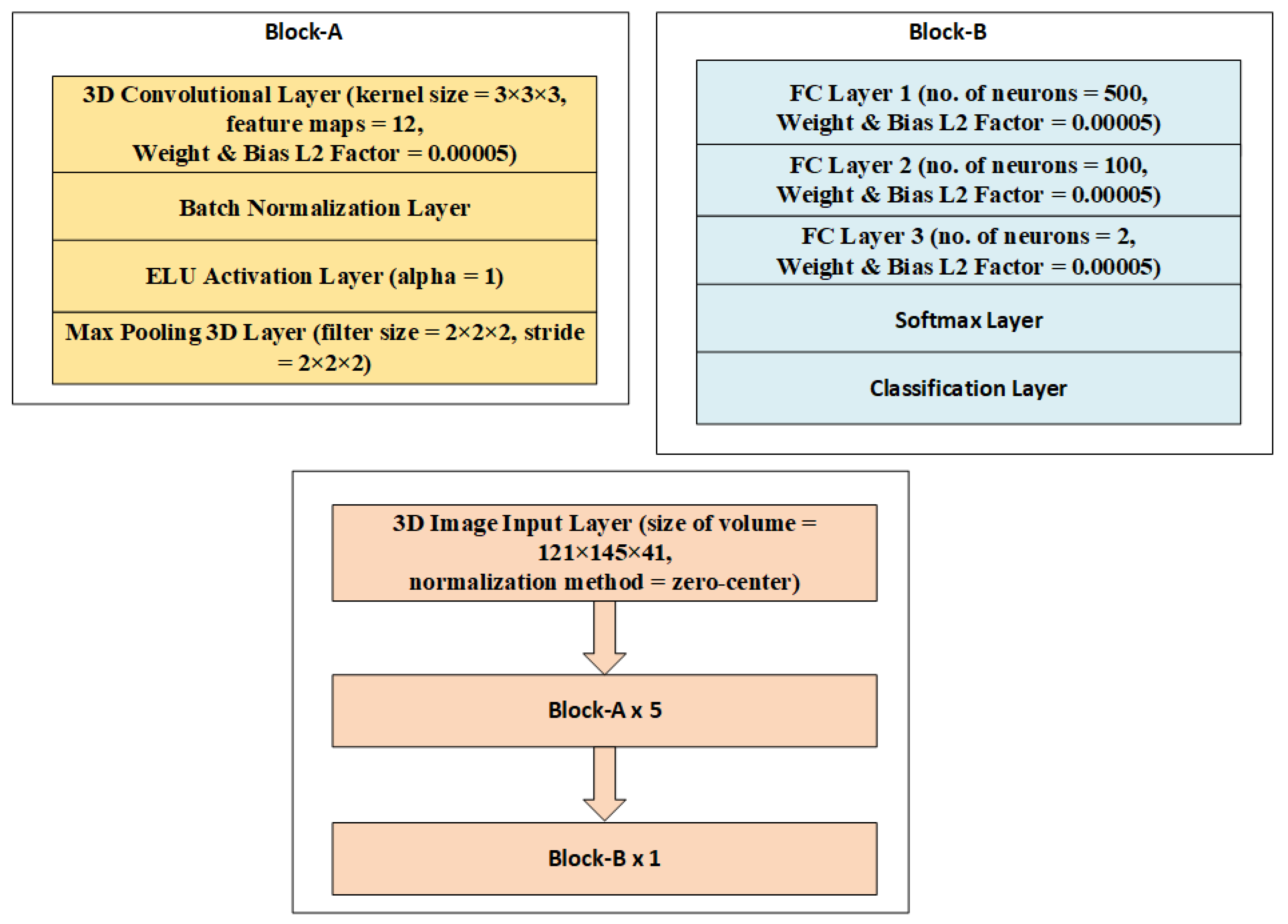
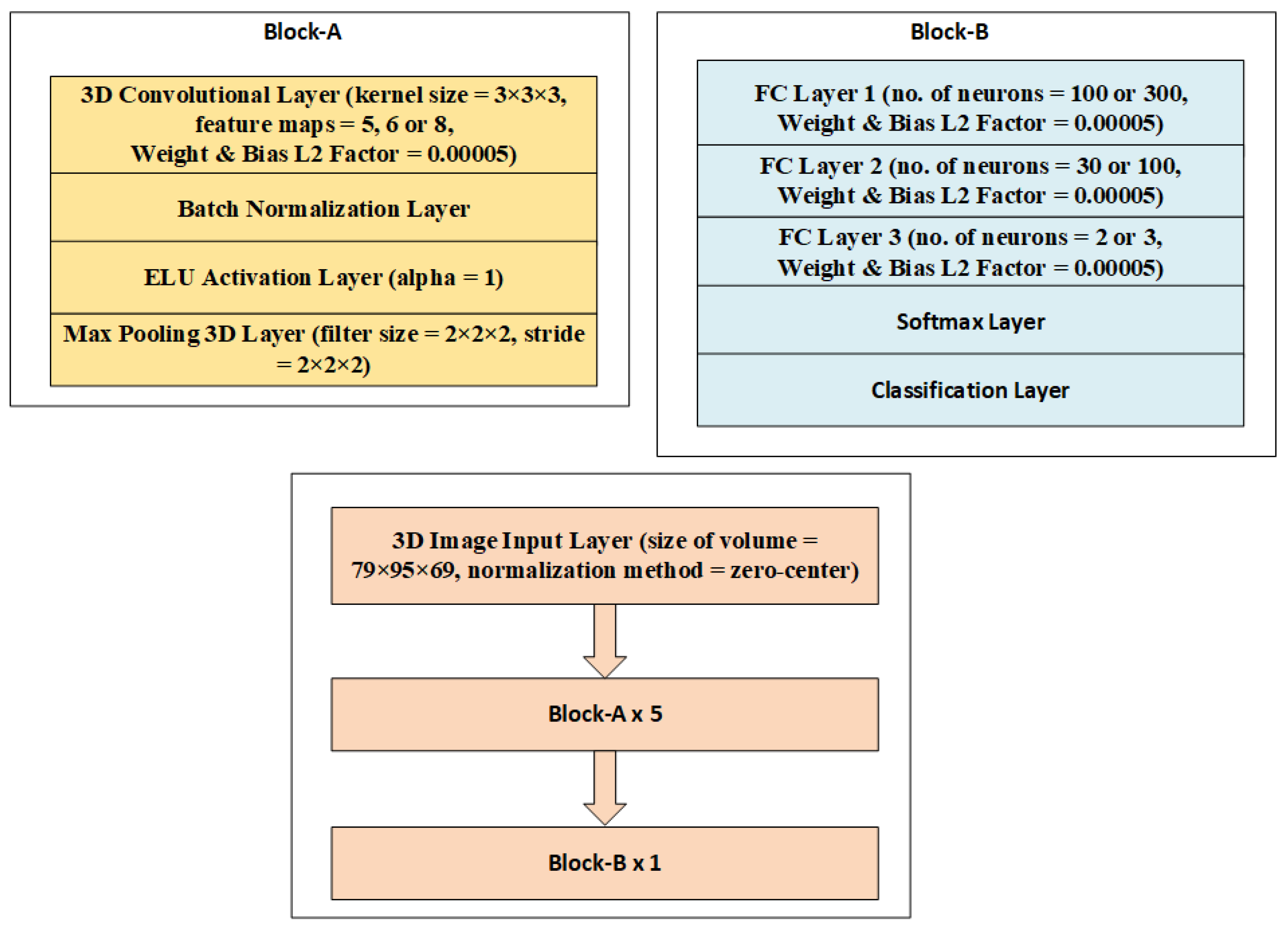
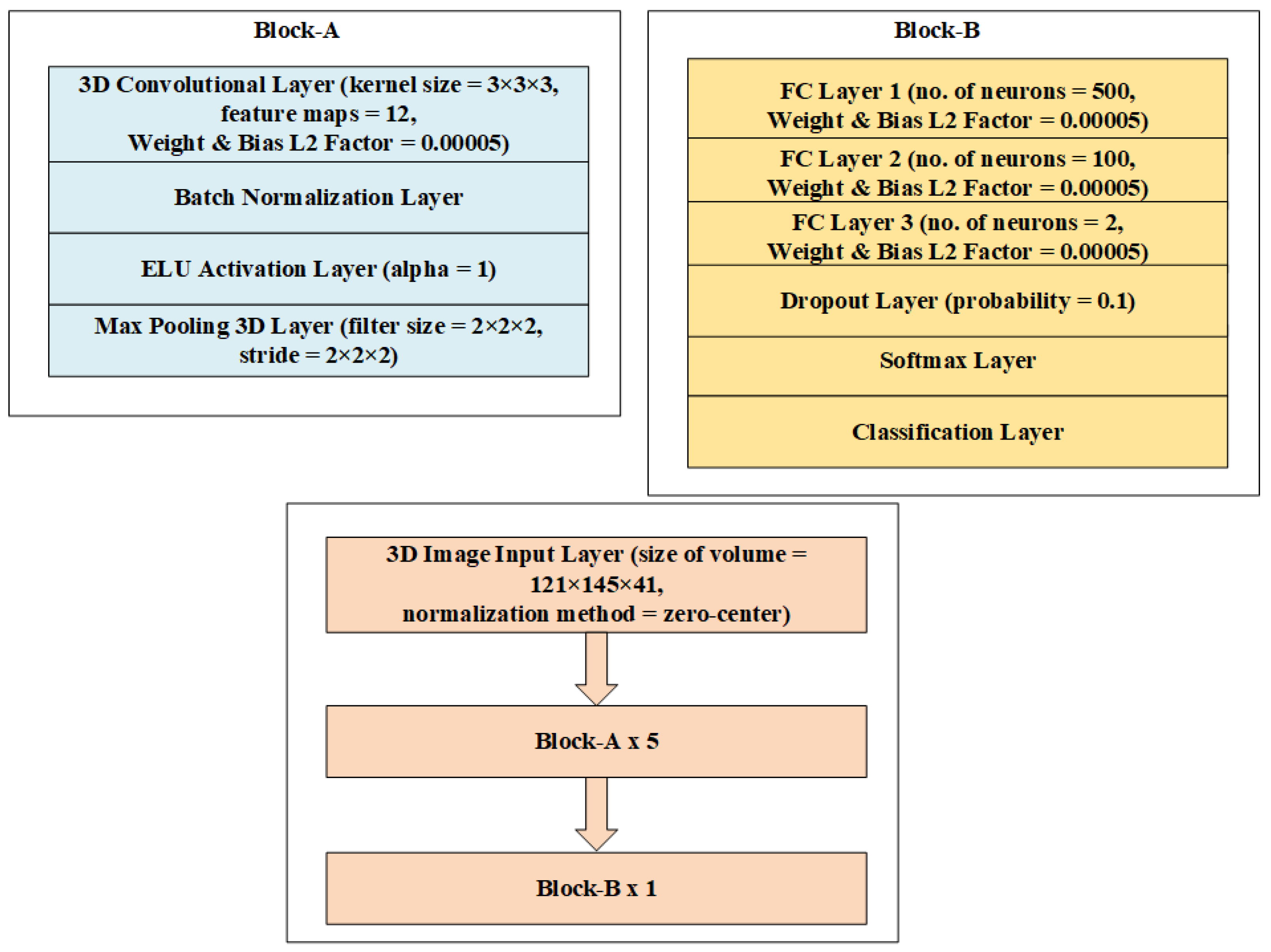
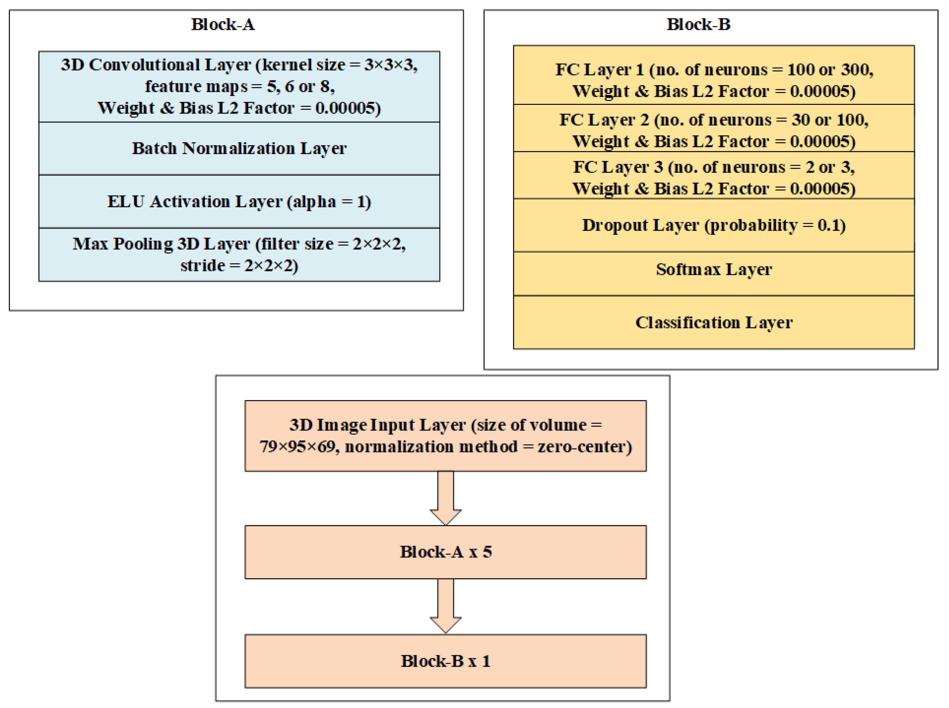
3. Methodology
4. Experiments and Results
5. Discussion
6. Conclusions
Author Contributions
Funding
Institutional Review Board Statement
Informed Consent Statement
Data Availability Statement
Conflicts of Interest
References
- Dubois, B.; Hampel, H.; Feldman, H.H.; Scheltens, P.; Aisen, P.; Andrieu, S.; Bakardjian, H.; Benali, H.; Bertram, L.; Blennow, K.; et al. Preclinical Alzheimer’s disease: Definition, natural history, and diagnostic criteria. Alzheimers Dement. 2016, 12, 292–323. [Google Scholar] [CrossRef] [PubMed]
- Cao, J.; Hou, J.; Ping, J.; Cai, D. Advances in developing novel therapeutic strategies for Alzheimer’s disease. Mol. Neurodegener. 2018, 13, 64. [Google Scholar] [PubMed] [Green Version]
- Slot, R.E.R.; Sikkes, S.A.M.; Berkhof, J.; Brodaty, H.; Buckley, R.; Cavedo, E.; Dardiotis, E.; Guillo-Benarous, F.; Hampel, H.; Kochan, N.A.; et al. Subjective cognitive decline and rates of incident Alzheimer’s disease and non-Alzheimer’s disease dementia. Alzheimers Dement. 2019, 15, 465–476. [Google Scholar] [CrossRef] [PubMed]
- Tufail, A.B.; Ma, Y.K.; Kaabar, M.K.; Martínez, F.; Junejo, A.R.; Ullah, I.; Khan, R. Deep learning in cancer diagnosis and prognosis prediction: A minireview on challenges, recent trends, and future directions. Comput. Math. Methods Med. 2021, 2021, 9025470. [Google Scholar]
- Khan, R.; Yang, Q.; Ullah, I.; Rehman, A.U.; Tufail, A.B.; Noor, A.; Cengiz, K. 3D convolutional neural networks based automatic modulation classification in the presence of channel noise. IET Commun. 2021, 16, 497–509. [Google Scholar] [CrossRef]
- Tufail, A.B.; Ma, Y.K.; Zhang, Q.N.; Khan, A.; Zhao, L.; Yang, Q.; Ullah, I. 3D convolutional neural networks-based multiclass classification of Alzheimer’s and Parkinson’s diseases using PET and SPECT neuroimaging modalities. Brain Inform. 2021, 8, 1–9. [Google Scholar]
- Ahmad, I.; Ullah, I.; Khan, W.U.; Rehman, A.U.; Adrees, M.S.; Saleem, M.Q.; Cheikhrouhou, O.; Hamam, H.; Shafiq, M. Efficient Algorithms for E-Healthcare to Solve Multiobject Fuse Detection Problem. J. Healthc. Eng. 2021, 2021, 9500304. [Google Scholar] [CrossRef]
- De Ture, M.A.; Dickson, D.W. The neuropathological diagnosis of Alzheimer’s disease. Mol. Neurodegener. 2019, 14, 32. [Google Scholar]
- Mukherjee, S.; Mez, J.; Trittschuh, E.H.; Saykin, A.J.; Gibbons, L.E.; Fardo, D.W.; Wessels, M.; Bauman, J.; Moore, M.; Choi, S.-E.; et al. Genetic data and cognitively-defined late-onset Alzheimer’s disease subgroups. Mol. Psychiatry 2019, 25, 2942–2951. [Google Scholar] [CrossRef] [Green Version]
- Edwards, G.A., III; Gamez, N.; Escobedo, G., Jr.; Calderon, O.; Moreno-Gonzalez, I. Modifiable Risk Factors for Alzheimer’s Disease. Front. Aging Neurosci. 2019, 11, 146. [Google Scholar]
- Mendez, M.F. Early-onset Alzheimer Disease and Its Variants. Continuum 2019, 25, 34–51. [Google Scholar] [CrossRef] [PubMed]
- Kim, M.; Snowden, S.; Suvitaival, T.; Ali, A.; Merkler, D.J.; Ahmad, T.; Westwood, S.; Baird, A.; Proitsi, P.; Nevado-Holgado, A.; et al. Primary fatty amides in plasma associated with brain amyloid burden, hippocampal volume, and memory in the European Medical Information Framework for Alzheimer’s Disease biomarker discovery cohort. Alzheimer’s Dement. 2019, 15, 817–827. [Google Scholar]
- Sundas, A.; Badotra, S.; Bharany, S.; Almogren, A.; Tag-ElDin, E.M.; Rehman, A.U. HealthGuard: An Intelligent Healthcare System Security Framework Based on Machine Learning. Sustainability 2022, 14, 11934. [Google Scholar] [CrossRef]
- Serrano-Pozo, A.; Growdon, J.H. Is Alzheimer’s Disease Risk Modifiable? J. Alzheimers Dis. 2019, 67, 795–819. [Google Scholar] [CrossRef] [PubMed]
- Rehman, A.U.; Naqvi, R.A.; Rehman, A.; Paul, A.; Sadiq, M.T.; Hussain, D. A Trustworthy SIoT Aware Mechanism as an Enabler for Citizen Services in Smart Cities. Electronics 2020, 9, 918. [Google Scholar] [CrossRef]
- Tufail, A.B.; Anwar, N.; Othman, M.T.; Ullah, I.; Khan, R.A.; Ma, Y.K.; Adhikari, D.; Rehman, A.U.; Shafiq, M.; Hamam, H. Early-stage Alzheimer’s disease categorization using PET neuroimaging modality and convolutional neural networks in the 2D and 3D domains. Sensors 2022, 22, 4609. [Google Scholar] [CrossRef]
- Ahmad, S.; Ullah, T.; Ahmad, I.; Al-Sharabi, A.; Ullah, K.; Khan, R.A.; Rasheed, S.; Ullah, I.; Uddin, M.; Ali, M. A novel hybrid deep learning model for metastatic cancer detection. Comput. Intell. Neurosci. 2022, 2022, 8141530. [Google Scholar]
- Basher, A.; Kim, B.C.; Lee, K.H.; Jung, H.Y. Volumetric Feature-Based Alzheimer’s Disease Diagnosis From sMRI Data Using a Convolutional Neural Network and a Deep Neural Network. IEEE Access 2021, 9, 29870–29882. [Google Scholar] [CrossRef]
- Martinez-Murcia, F.J.; Ortiz, A.; Gorriz, J.-M.; Ramirez, J.; Castillo-Barnes, D. Studying the Manifold Structure of Alzheimer’s Disease: A Deep Learning Approach Using Convolutional Autoencoders. IEEE J. Biomed. Health Inform. 2020, 24, 17–26. [Google Scholar] [CrossRef]
- Murugan, S.; Venkatesan, C.; Sumithra, M.G.; Gao, X.-Z.; Elakkiya, B.; Akila, M.; Manoharan, S. DEMNET: A Deep Learning Model for Early Diagnosis of Alzheimer Diseases and Dementia from MR Images. IEEE Access 2021, 9, 90319–90329. [Google Scholar] [CrossRef]
- Tanveer, M.; Rashid, A.H.; Ganaie, M.A.; Reza, M.; Razzak, I.; Hua, K.-L. Classification of Alzheimer’s disease using ensemble of deep neural networks trained through transfer learning. IEEE J. Biomed. Health Inform. 2021, 26, 1453–1463. [Google Scholar] [CrossRef]
- Tufail, A.B.; Ullah, I.; Khan, R.; Ali, L.; Yousaf, A.; Rehman, A.U.; Ma, Y.K. Recognition of Ziziphus lotus through Aerial Imaging and Deep Transfer Learning Approach. Mob. Inf. Syst. 2021, 2021, 4310321. [Google Scholar] [CrossRef]
- Yousafzai, B.K.; Khan, S.A.; Rahman, T.; Khan, I.; Ullah, I.; Ur Rehman, A.; Cheikhrouhou, O. Student-performulator: Student academic performance using hybrid deep neural network. Sustainability 2021, 13, 9775. [Google Scholar]
- Sadiq, M.T.; Yu, X.; Yuan, Z.; Zeming, F.; Rehman, A.U.; Ullah, I.; Li, G.; Xiao, G. Motor imagery EEG signals decoding by multivariate empirical wavelet transform-based framework for robust brain–computer interfaces. IEEE Access 2019, 7, 171431–171451. [Google Scholar]
- Bin Tufail, A.; Ullah, I.; Khan, W.U.; Asif, M.; Ahmad, I.; Ma, Y.-K.; Khan, R.; Kalimullah; Ali, S. Diagnosis of Diabetic Retinopathy through Retinal Fundus Images and 3D Convolutional Neural Networks with Limited Number of Samples. Wirel. Commun. Mob. Comput. 2021, 2021, 6013448. [Google Scholar] [CrossRef]
- Mahendran, N.; PM, D.R. A deep learning framework with an embedded based feature selection approach for the early detection of the Alzheimer’s disease. Comput. Biol. Med. 2022, 141, 105056. [Google Scholar]
- Han, R.; Chen, C.L.P.; Liu, Z. A Novel Convolutional Variation of Broad Learning System for Alzheimer’s Disease Diagnosis by Using MRI Images. IEEE Access 2020, 8, 214646–214657. [Google Scholar] [CrossRef]
- Lu, B.; Li, H.X.; Chang, Z.K.; Li, L.; Chen, N.X.; Zhu, Z.C.; Zhou, H.X.; Li, X.Y.; Wang, Y.W.; Cui, S.X.; et al. A practical Alzheimer’s disease classifier via brain imaging-based deep learning on 85,721 samples. J. Big Data 2022, 9, 101. [Google Scholar] [CrossRef]
- Syed, A.H.; Khan, T.; Hassan, A.; Alromema, N.A.; Binsawad, M.; Alsayed, A.O. An Ensemble-Learning Based Application to Predict the Earlier Stages of Alzheimer’s Disease (AD). IEEE Access 2020, 8, 222126–222143. [Google Scholar] [CrossRef]
- Saleem, T.J.; Zahra, S.R.; Wu, F.; Alwakeel, A.; Alwakeel, M.; Jeribi, F.; Hijji, M. Deep Learning-Based Diagnosis of Alzheimer’s Disease. J. Pers. Med. 2022, 12, 815. [Google Scholar] [CrossRef]
- Yuan, S.; Li, H.; Wu, J.; Sun, X. Classification of Mild Cognitive Impairment with Multimodal Data using both Labeled and Unlabeled Samples. IEEE/ACM Trans. Comput. Biol. Bioinform. 2021, 18, 2281–2290. [Google Scholar] [CrossRef] [PubMed]
- Assam, M.; Kanwal, H.; Farooq, U.; Shah, S.K.; Mehmood, A.; Choi, G.S. An Efficient Classification of MRI Brain Images. IEEE Access 2021, 9, 33313–33322. [Google Scholar] [CrossRef]
- Zhang, F.; Pan, B.; Shao, P.; Liu, P.; Shen, S.; Yao, P.; Xu, R.X. A Single Model Deep Learning Approach for Alzheimer’s Disease Diagnosis. Neuroscience 2022, 491, 200–214. [Google Scholar] [PubMed]
- Guo, H.; Zhang, Y. Resting State fMRI and Improved Deep Learning Algorithm for Earlier Detection of Alzheimer’s Disease. IEEE Access 2020, 8, 115383–115392. [Google Scholar] [CrossRef]
- Santurkar, S.; Tsipras, D.; Ilyas, A.; Madry, A. How Does Batch Normalization Help Optimization? arXiv 2019, arXiv:1805.11604v5. [Google Scholar]
- Bjorck, J.; Gomes, C.; Selman, B.; Weinberger, K.Q. Understanding Batch Normalization. arXiv 2018, arXiv:1806.02375v4. [Google Scholar]
- Ioffe, S.; Szegedy, C. Batch Normalization: Accelerating Deep Network Training by Reducing Internal Covariate Shift. arXiv 2015, arXiv:1502.03167v3. [Google Scholar]
- Daneshmand, H.; Joudaki, A.; Bach, F. Batch Normalization orthogonalizes representations in deep random networks. Adv. Neural Inf. Process. Syst. 2021, 34, 4896–4906. [Google Scholar]
- Srivastava, N.; Hinton, G.; Krizhevsky, A.; Sutskever, I.; Salakhutdinov, R. Dropout: A Simple Way to Prevent Neural Networks from Overfitting. J. Mach. Learn. Res. 2014, 15, 1929–1958. [Google Scholar]
- Labach, A.; Salehinejad, H.; Valaee, S. Survey of Dropout Methods for Deep Neural Networks. arXiv 2019, arXiv:1904.13310v2. [Google Scholar]
- Fan, X.; Zhang, S.; Tanwisuth, K.; Qian, X.; Zhou, M. Contextual dropout: An efficient sample dependent dropout module. arXiv 2021, arXiv:2103.04181v1. [Google Scholar]
- Xie, J.; Ma, Z.; Lei, J.; Zhang, G.; Xue, J.-H.; Tan, Z.-H.; Guo, J. Advanced Dropout: A Model-free Methodology for Bayesian Dropout Optimization. arXiv 2021, arXiv:2010.05244v2. [Google Scholar]
- Li, X.; Chen, S.; Hu, X.; Yang, J. Understanding the Disharmony between Dropout and Batch Normalization by Variance Shift. In Proceedings of the 2019 IEEE/CVF Conference on Computer Vision and Pattern Recognition (CVPR), Long Beach, CA, USA, 15–20 June 2019; pp. 2677–2685. [Google Scholar] [CrossRef] [Green Version]
- Weiner, M.W.; Aisen, P.S.; Jack, C.R., Jr.; Jagust, W.J.; Trojanowski, J.Q.; Shaw, L.; Saykin, A.J.; Morris, J.C.; Cairns, N.; Beckett, L.A.; et al. The Alzheimer’s disease Neuroimaging Initiative: Progress report and future plans. Alzheimers. Dement. 2010, 6, 202–211. [Google Scholar] [CrossRef] [PubMed] [Green Version]
- Wen, J.; Thibeau-Sutre, E.; Diaz-Melo, M.; Samper-González, J.; Routier, A.; Bottani, S.; Dormont, D.; Durrleman, S.; Burgos, N.; Colliot, O. Convolutional neural networks for classification of Alzheimer’s disease: Overview and reproducible evaluation. Med. Image Anal. 2020, 63, 101694. [Google Scholar] [CrossRef] [PubMed]
- Spasov, S.; Passamonti, L.; Duggento, A.; Liò, P.; Toschi, N.; for the Alzheimer's Disease Neuroimaging Initiative. A parameter-efficient deep learning approach to predict conversion from mild cognitive impairment to Alzheimer’s disease. Neuroimage 2019, 189, 276–287. [Google Scholar] [CrossRef] [Green Version]
- Tufail, A.B.; Ma, Y.-K.; Kaabar, M.K.A.; Rehman, A.U.; Khan, R.; Cheikhrouhou, O. Classification of Initial Stages of Alzheimer’s Disease through Pet Neuroimaging Modality and Deep Learning: Quantifying the Impact of Image Filtering Approaches. Mathematics 2021, 9, 3101. [Google Scholar] [CrossRef]
- Zhu, T.; Cao, C.; Wang, Z.; Xu, G.; Qiao, J. Anatomical Landmarks and DAG Network Learning for Alzheimer’s Disease Diagnosis. IEEE Access 2020, 8, 206063–206073. [Google Scholar] [CrossRef]
- Choi, J.Y.; Lee, B. Combining of Multiple Deep Networks via Ensemble Generalization Loss, Based on MRI Images, for Alzheimer’s Disease Classification. IEEE Signal Process. Lett. 2020, 27, 206–210. [Google Scholar] [CrossRef]
- Basheer, S.; Bhatia, S.; Sakri, S.B. Computational Modeling of Dementia Prediction Using Deep Neural Network: Analysis on OASIS Dataset. IEEE Access 2021, 9, 42449–42462. [Google Scholar] [CrossRef]
- Lian, C.; Liu, M.; Zhang, J.; Shen, D. Hierarchical Fully Convolutional Network for Joint Atrophy Localization and Alzheimer’s Disease Diagnosis Using Structural MRI. IEEE Trans. Pattern Anal. Mach. Intell. 2020, 42, 880–893. [Google Scholar] [CrossRef]
- Er, F.; Goularas, D. Predicting the Prognosis of MCI Patients Using Longitudinal MRI Data. IEEE/ACM Trans. Comput. Biol. Bioinform. 2021, 18, 1164–1173. [Google Scholar] [PubMed]
- Xia, Z.; Zhou, T.; Mamoon, S.; Lu, J. Recognition of Dementia Biomarkers with Deep Finer-DBN. IEEE Trans. Neural Syst. Rehabil. Eng. 2021, 29, 1926–1935. [Google Scholar] [CrossRef] [PubMed]
- Cuingnet, R.; Gerardin, E.; Tessieras, J.; Auzias, G.; Lehéricy, S.; Habert, M.-O.; Chupin, M.; Benali, H.; Colliot, O. Automatic classification of patients with Alzheimer’s disease from structural MRI: A comparison of ten methods using the ADNI database. Neuroimage 2011, 56, 766–781. [Google Scholar] [PubMed] [Green Version]
- Bin Tufail, A.; Ullah, K.; Khan, R.A.; Shakir, M.; Khan, M.A.; Ullah, I.; Ma, Y.-K.; Ali, S. On Improved 3D-CNN-Based Binary and Multiclass Classification of Alzheimer’s Disease Using Neuroimaging Modalities and Data Augmentation Methods. J. Healthc. Eng. 2022, 2022, 1302170. [Google Scholar] [CrossRef]
- Aderghal, K.; Afdel, K.; Benois-Pineau, J.; Catheline, G. Improving Alzheimer’s stage categorization with Convolutional Neural Network using transfer learning and different magnetic resonance imaging modalities. Heliyon 2020, 6, e05652. [Google Scholar] [CrossRef]
- Oh, K.; Chung, Y.C.; Kim, K.W.; Kim, W.S.; Oh, I.S. Author correction: Classification and visualization of Alzheimer’s disease using volumetric convolutional neural network and transfer learning. Sci. Rep. 2020, 10, 5663. [Google Scholar]
- Yagis, E.; Citi, L.; Diciotti, S.; Marzi, C.; Atnafu, S.W.; De Herrera, A.G.S. 3D Convolutional Neural Networks for Diagnosis of Alzheimer’s Disease via Structural MRI. In Proceedings of the 2020 IEEE 33rd International Symposium on Computer-Based Medical Systems, CBMS, Rochester, MN, USA, 28–30 July 2020. [Google Scholar]
- Ieracitano, C.; Mammone, N.; Hussain, A.; Morabito, F.C. A Convolutional Neural Network based self-learning approach for classifying neurodegenerative states from EEG signals in dementia. In Proceedings of the 2020 International Joint Conference on Neural Networks, IJCNN, Glasgow, UK, 19–24 July 2020. [Google Scholar]
- Prajapati, R.; Khatri, U.; Kwon, G.R. An Efficient Deep Neural Network Binary Classifier for Alzheimer’s disease Classification. In Proceedings of the 2021 International Conference on Artificial Intelligence in Information and Communication, ICAIIC, Jeju Island, Korea, 20–23 April 2021. [Google Scholar]
- Tomassini, S.; Falcionelli, N.; Sernani, P.; Müller, H.; Dragoni, A.F. An End-to-End 3D ConvLSTM-based Framework for Early Diagnosis of Alzheimer’s Disease from Full-Resolution Whole-Brain sMRI Scans. In Proceedings of the 2021 IEEE 34th International Symposium on Computer-Based Medical Systems, CBMS, Aveiro, Portugal, 7–9 June 2021. [Google Scholar]
- Rejusha, T.R.; Vipin Kumar, K.S. Artificial MRI Image Generation using Deep Convolutional GAN and its Comparison with other Augmentation Methods. In Proceedings of the 2021 International Conference on Communication, Control and Information Sciences, ICCISc, Idukki, India, 16–18 June 2021. [Google Scholar]
- Yagis, E.; de Herrera, A.G.S.; Citi, L. Convolutional Autoencoder based Deep Learning Approach for Alzheimer’s Disease Diagnosis using Brain MRI. In Proceedings of the 2021 IEEE 34th International Symposium on Computer-Based Medical Systems, CBMS, Aveiro, Portugal, 7–9 June 2021. [Google Scholar]
- Sarasua, I.; Lee, J.; Wachinger, C. Geometric Deep Learning on Anatomical Meshes for the Prediction of Alzheimer’s disease. In Proceedings of the 2021 IEEE 18th International Symposium on Biomedical Imaging, ISBI, Nice, France, 13–16 April 2021. [Google Scholar]
- Kaur, S.; Sharma, S.; Rehman, A.U.; Eldin, E.T.; Ghamry, N.A.; Shafiq, M.; Bharany, S. Predicting Infection Positivity, Risk Estimation, and Disease Prognosis in Dengue Infected Patients by ML Expert System. Sustainability 2022, 14, 13490. [Google Scholar] [CrossRef]
- Aderghal, K.; Boissenin, M.; Benois-Pineau, J.; Catheline, G.; Afdel, K. Classification of sMRI for AD Diagnosis with Convolutional Neuronal Networks: A Pilot 2-D+ɛ Study on ADNI. In Proceedings of the International Conference on Multimedia Modeling, Reykjavik, Iceland, 4–6 January 2017. [Google Scholar]
- Aderghal, K.; Benois-Pineau, J.; Afdel, K. FuseMe: Classification of sMRI images by fusion of Deep CNNs in 2D+ε projections. In Proceedings of the International Workshop on Content-Based Multimedia Indexing, CBMI, Florence, Italy, 19–21 June 2017. [Google Scholar]
- Kam, T.E.; Zhang, H.; Jiao, Z.; Shen, D. Deep Learning of Static and Dynamic Brain Functional Networks for Early MCI Detection. IEEE Trans. Med. Imaging 2020, 39, 478–487. [Google Scholar] [CrossRef]
- Ben Ahmed, O.; Mizotin, M.; Benois-Pineau, J.; Allard, M.; Catheline, G.; Ben Amar, C. Alzheimer’s disease diagnosis on structural MR images using circular harmonic functions descriptors on hippocampus and posterior cingulate cortex. Comput. Med. Imaging Graph. 2015, 44, 13–25. [Google Scholar]
- Khagi, B.; Kwon, G.-R. 3D CNN Design for the Classification of Alzheimer’s Disease Using Brain MRI and PET. IEEE Access 2020, 8, 217830–217847. [Google Scholar] [CrossRef]
- Puspaningrum, E.Y.; Wahid, R.R.; Amaliyah, R.P. Alzheimer’s Disease Stage Classification using Deep Convolutional Neural Networks on Oversampled Imbalance Data. In Proceedings of the 2020 6th Information Technology International Seminar, ITIS, Surabaya, Indonesia, 14–16 October 2020. [Google Scholar]


| Demographics | NC | MCI | AD |
|---|---|---|---|
| Subjects | 102 | 97 | 94 |
| Age | 76.01 (62.21–86.62) | 74.54 (55.32–87.23) | 75.82 (55.32–881) |
| Weight | 75.72 (49–130.3) | 77.13 (45.1–120.2) | 74.12 (42.62–127.54) |
| Functional Activities Questionnaire Total Score | 0.1863 (0–6) | 3.163 (0–15) | 13.672 (0–27) |
| Neuropsychiatric Inventory Questionnaire Total Score | 0.4023 (0–5) | 1.973 (0–17) | 4.0741 (0–15) |
| Demographics | NC | AD |
|---|---|---|
| Subjects Number | 228 | 187 |
| Age | 75.97 (60.02–89.74) | 75.4 (55.18–90.99) |
| Weight | 75.91 (45.81–137.44) | 72.03 (37.65–127.46) |
| Mini-Mental State Examination Score | 29.11 (25–30) | 23.26 (18–27) |
| Clinical Dementia Rating Global Score | 0 (0–0) | 0.75 (0.5–1) |
| Architecture Used | Metrics of Performance |
|---|---|
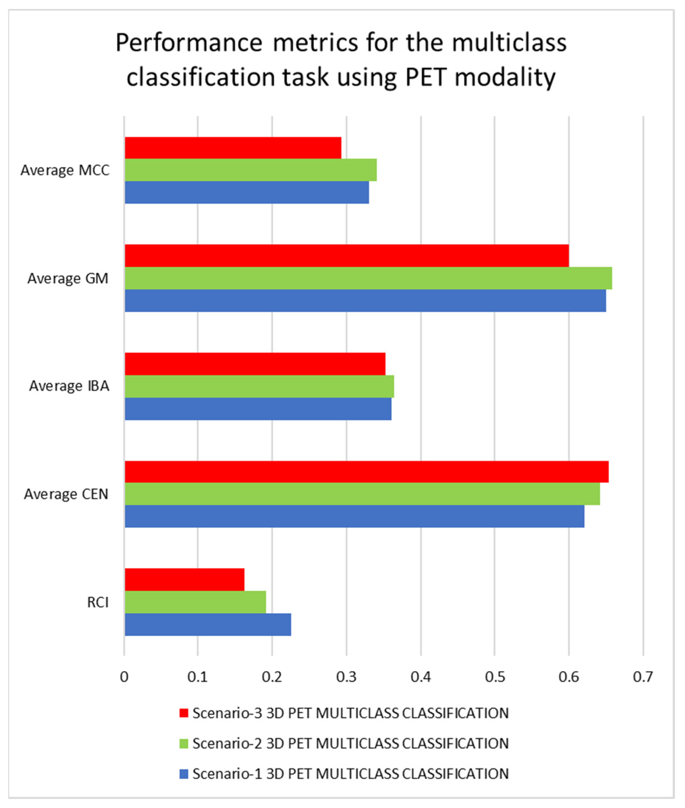
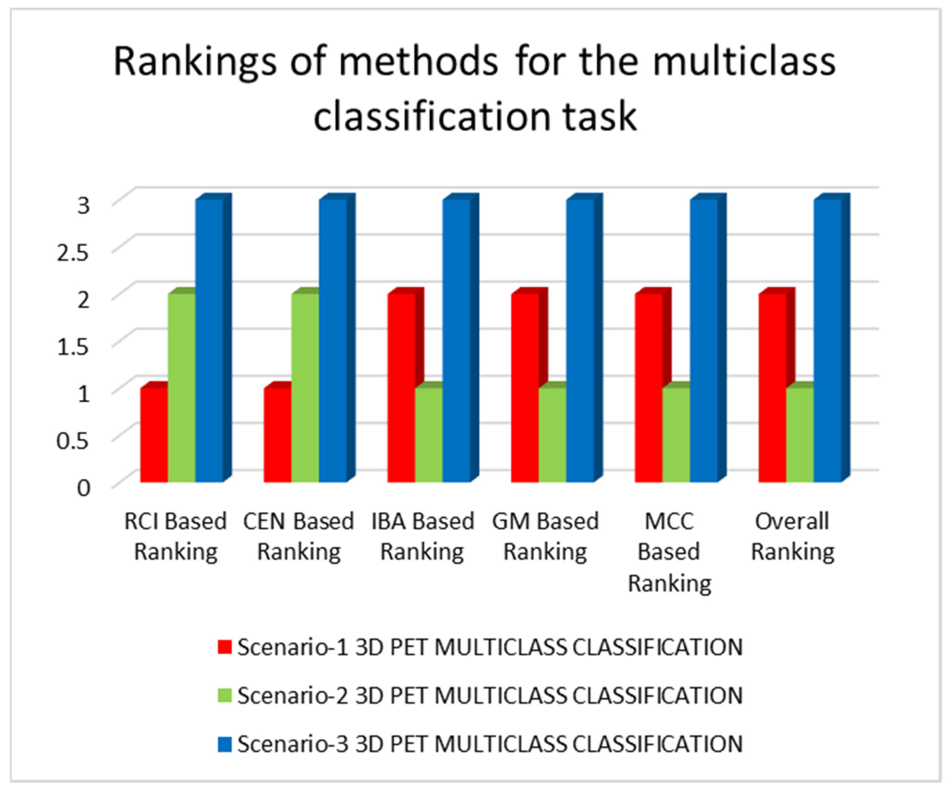
| 3D-CNN applying PET data to study scenario-1 | RCI = 0.2261, CEN = {‘AD’: 0.5054, ‘MCI’: 0.8572, ‘NC’: 0.4996}, Average CEN = 0.6207, IBA = {‘AD’: 0.4539, ‘MCI’: 0.1316, ‘NC’: 0.4969}, Average IBA = 0.3608, GM = {‘AD’: 0.7484, ‘MCI’: 0.4683, ‘NC’: 0.7344}, Average GM = 0.6503, MCC = {‘AD’: 0.5118, ‘MCI’: 0.019, ‘NC’: 0.4601}, Average MCC = 0.3303 |
| 3D-CNN applying PET data to study scenario-2 | RCI = 0.1923, CEN = {‘AD’: 0.5448, ‘MCI’: 0.8405, ‘NC’: 0.5407}, Average CEN = 0.642, IBA = {‘AD’: 0.4674, ‘MCI’: 0.1516, ‘NC’: 0.4734}, Average IBA = 0.3641, GM = {‘AD’: 0.7454, ‘MCI’: 0.4982, ‘NC’: 0.7289}, Average GM = 0.6575, MCC = {‘AD’: 0.4953, ‘MCI’: 0.0721, ‘NC’: 0.4543}, Average MCC = 0.3405 |
| 3D-CNN applying PET data to study scenario-3 | RCI = 0.1628, CEN = {‘AD’: 0.5692, ‘MCI’: 0.8398, ‘NC’: 0.5501}, Average CEN = 0.653, IBA = {‘AD’: 0.4407, ‘MCI’: 0.0411, ‘NC’: 0.5748}, Average IBA = 0.3522, GM = {‘AD’: 0.7424, ‘MCI’: 0.3597, ‘NC’: 0.6975}, Average GM = 0.5998, MCC = {‘AD’: 0.5026, ‘MCI’: −0.011, ‘NC’: 0.3881}, Average MCC = 0.2932 |
| Architecture Used | Metrics of Performance |
|---|---|
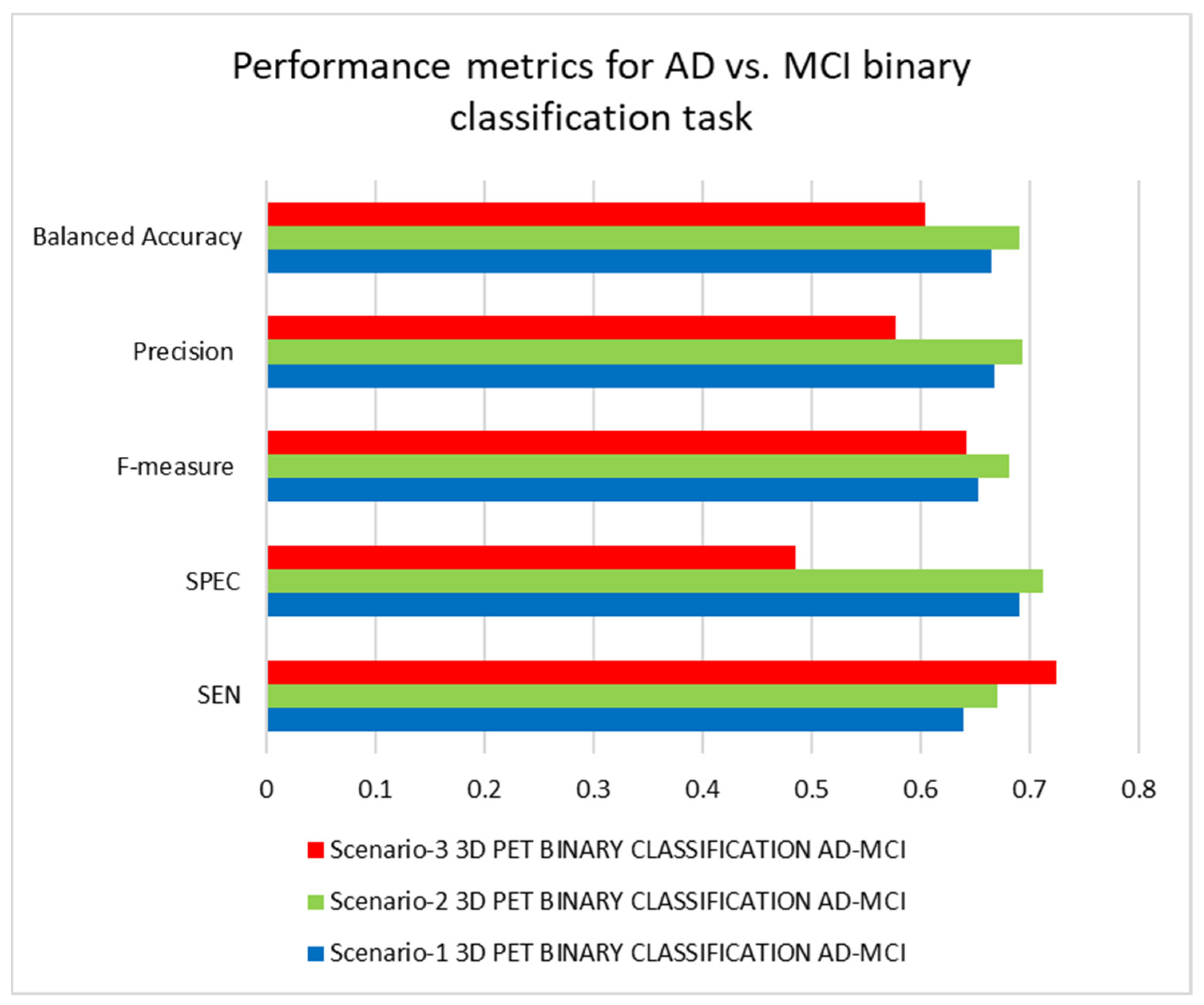
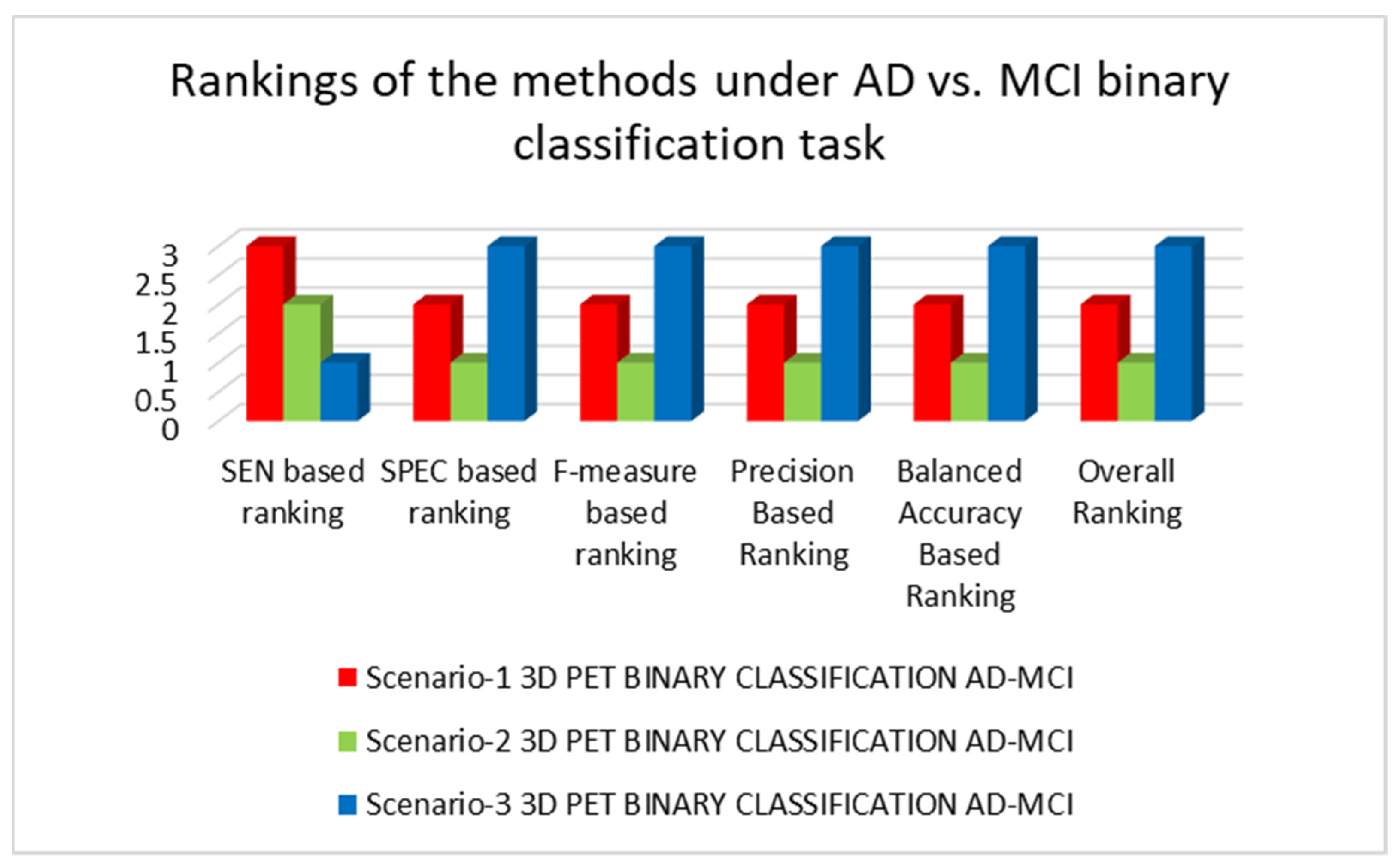
| 3D-CNN applying PET data to study scenario-1 | SEN = 0.6383, SPEC = 0.6907, F-measure = 0.6522, Precision = 0.6667, Balanced Accuracy = 0.6645 |
| 3D-CNN applying PET data to study scenario-2 | SEN = 0.6702, SPEC = 0.7113, F-measure = 0.6811, Precision = 0.6923, Balanced Accuracy = 0.6908 |
| 3D-CNN applying PET data to study scenario-3 | SEN = 0.7234, SPEC = 0.4845, F-measure = 0.6415, Precision = 0.5763, Balanced Accuracy = 0.6040 |
| Architecture | Performance Metrics |
|---|---|
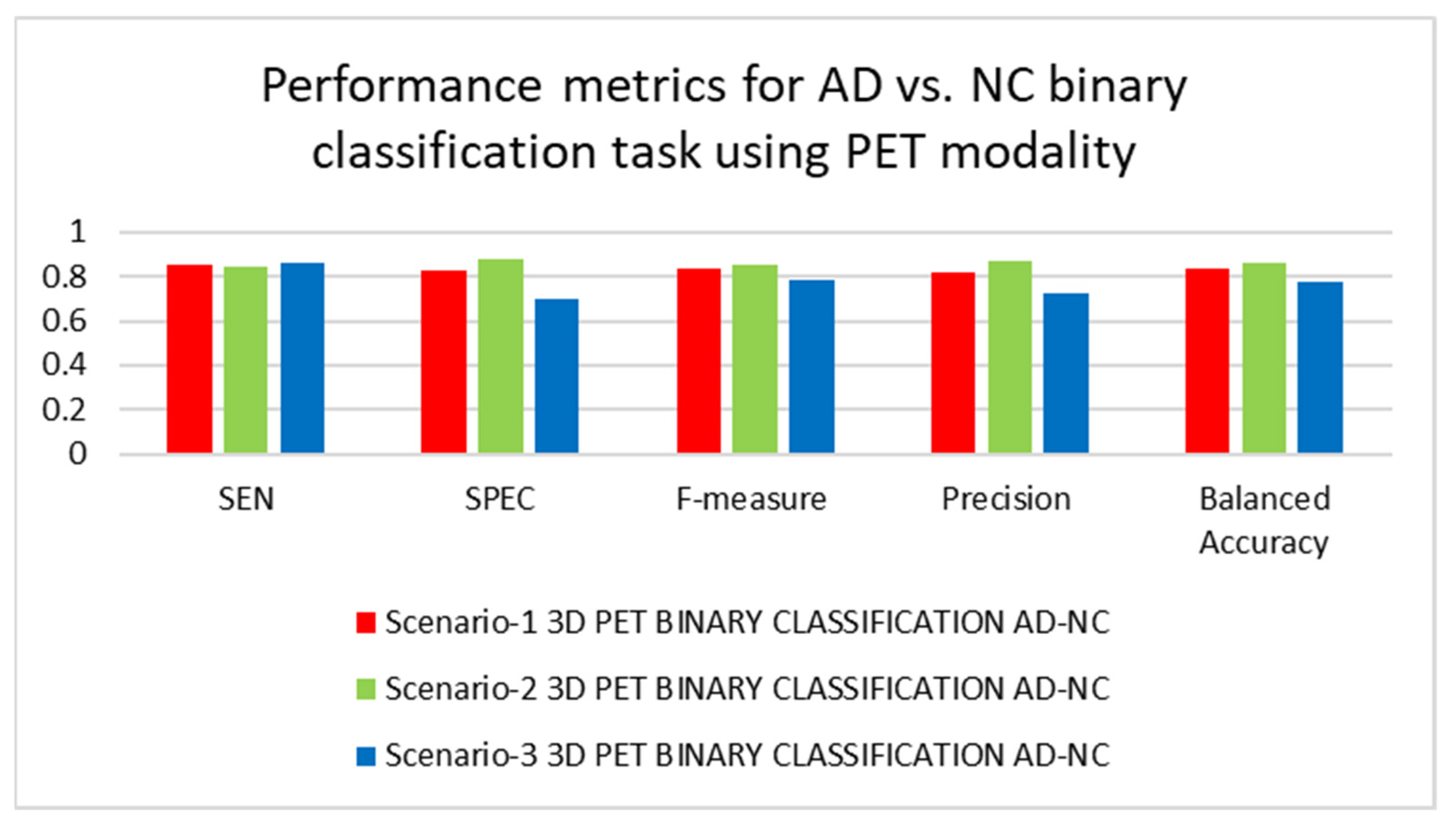
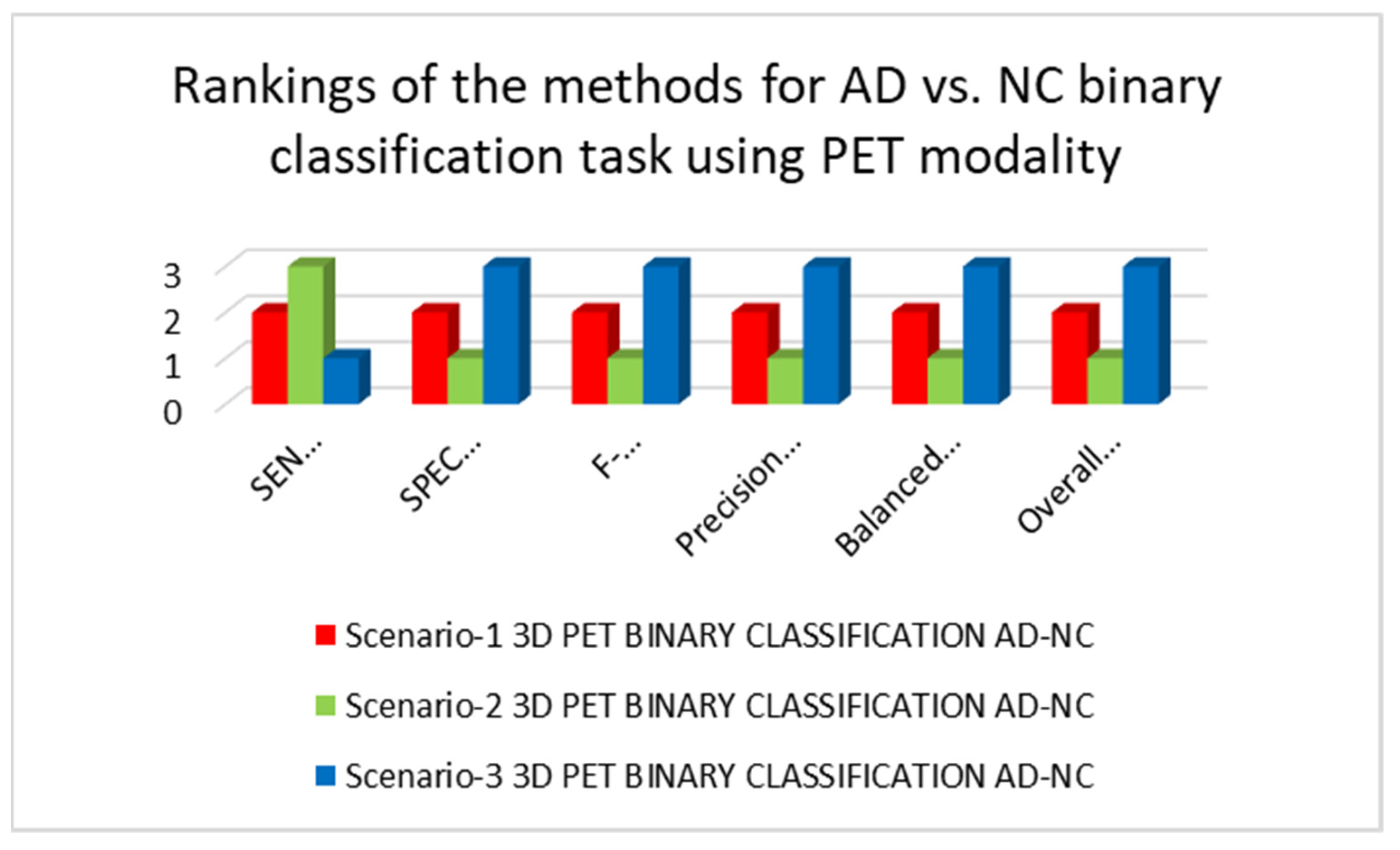
| 3D-CNN applying PET data to study scenario-1 | SEN = 0.8511, SPEC = 0.8235, F-measure = 0.8333, Precision = 0.8163, Balanced Accuracy = 0.8373 |
| 3D-CNN applying PET data to study scenario-2 | SEN = 0.8404, SPEC = 0.8824, F-measure = 0.8541, Precision = 0.8681, Balanced Accuracy = 0.8614 |
| 3D-CNN applying PET data to study scenario-3 | SEN = 0.8617, SPEC = 0.6961, F-measure = 0.7864, Precision = 0.7232, Balanced Accuracy = 0.7789 |
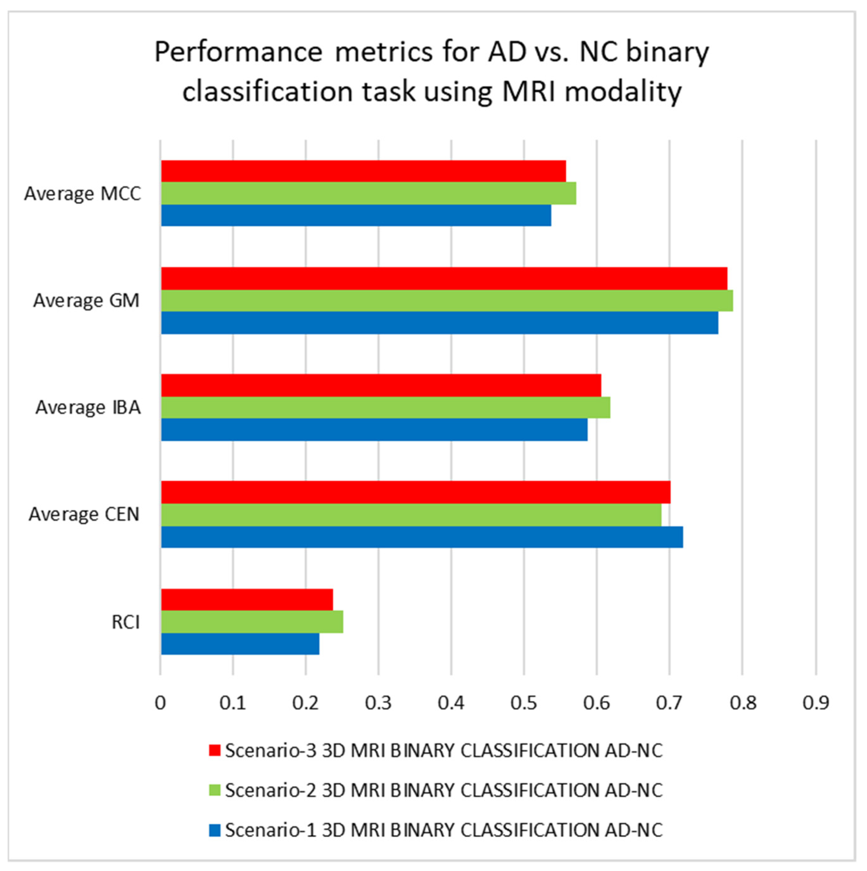
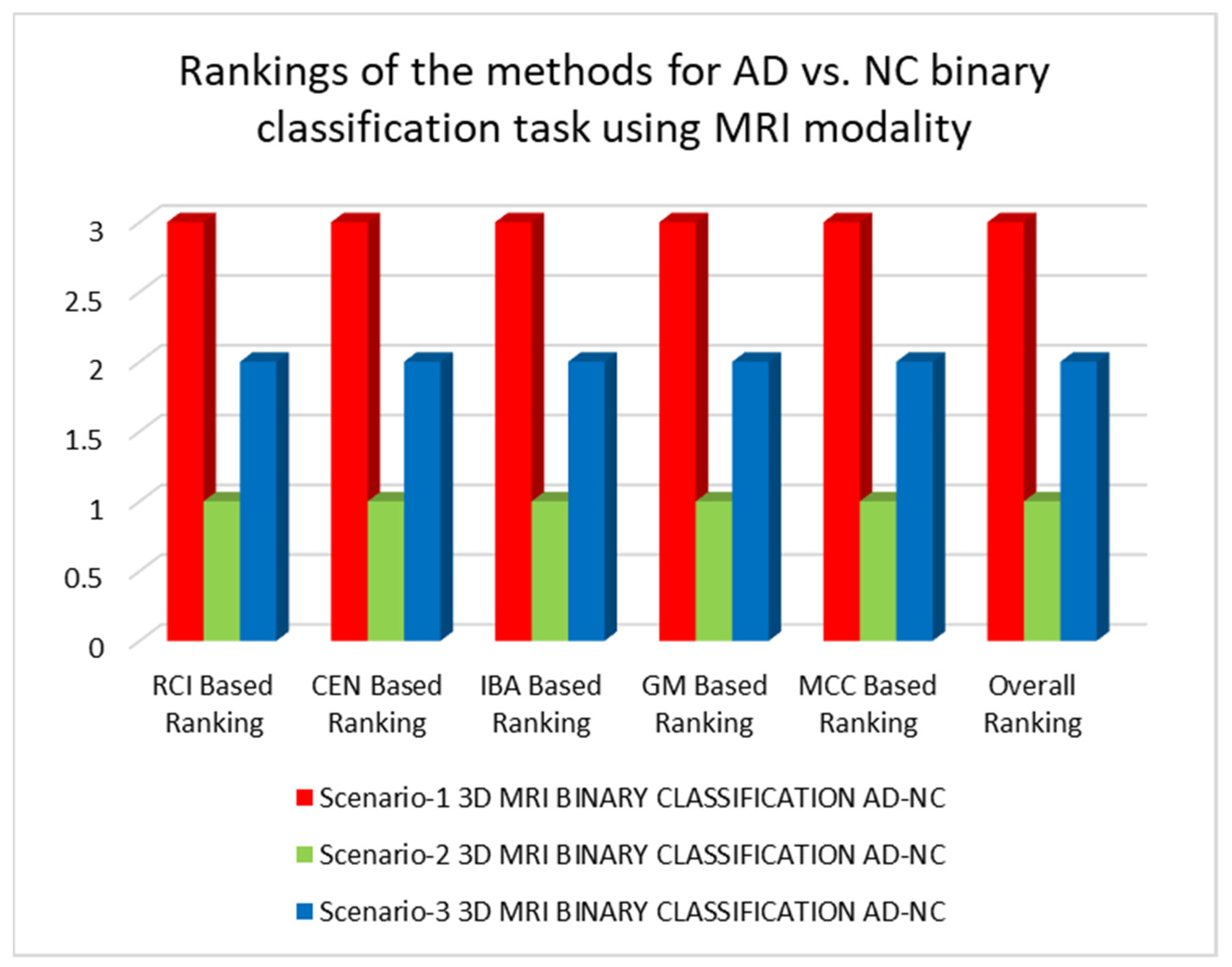
| 3D-CNN applying MRI data to study scenario-1 | RCI = 0.2194, CEN = {‘AD’: 0.7609, ‘NC’: 0.6752}, Average CEN = 0.71805, IBA = {‘AD’: 0.5468, ‘NC’: 0.6291}, Average IBA = 0.5879, GM = {‘AD’: 0.7668, ‘NC’: 0.7668}, Average GM = 0.7668, MCC = {‘AD’: 0.5367, ‘NC’: 0.5367}, Average MCC = 0.5367 |
| 3D-CNN applying MRI data to study scenario-2 | RCI = 0.2517, CEN = {‘AD’: 0.7243, ‘NC’: 0.6525}, Average CEN = 0.6884, IBA = {‘AD’: 0.5979, ‘NC’: 0.6382}, Average IBA = 0.618, GM = {‘AD’: 0.7861, ‘NC’: 0.7861}, Average GM = 0.7861, MCC = {‘AD’: 0.5721, ‘NC’: 0.5721}, Average MCC = 0.5721 |
| 3D-CNN applying MRI data to study scenario-3 | RCI = 0.238, CEN = {‘AD’: 0.7384, ‘NC’: 0.6643}, Average CEN = 0.7014, IBA = {‘AD’: 0.5825, ‘NC’: 0.6297}, Average IBA = 0.6061, GM = {‘AD’: 0.7785, ‘NC’: 0.7785}, Average GM = 0.7785, MCC = {‘AD’: 0.5573, ‘NC’: 0.5573}, Average MCC = 0.5573 |
| Architecture | Performance Metrics |
|---|---|
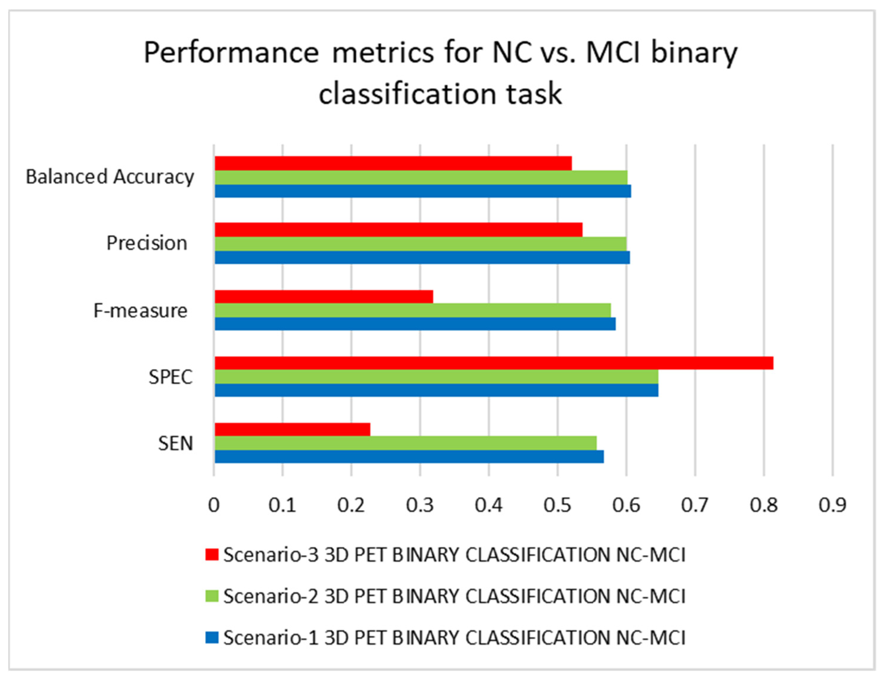
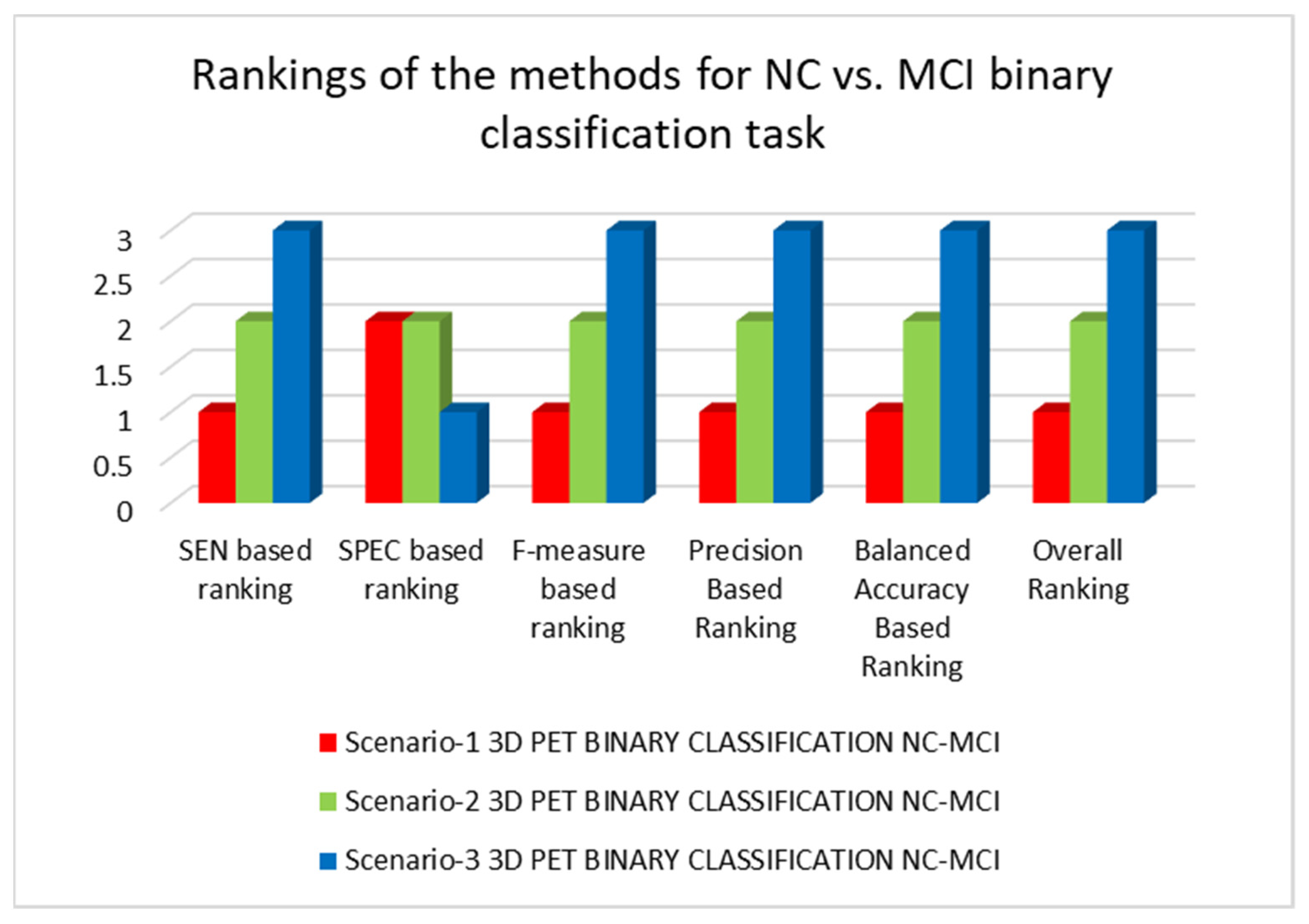
| 3D-CNN applying PET data to study scenario-1 | SEN = 0.5670, SPEC = 0.6471, F-measure = 0.5851, Precision = 0.6044, Balanced Accuracy = 0.6070 |
| 3D-CNN applying PET data to study scenario-2 | SEN = 0.5567, SPEC = 0.6471, F-measure = 0.5775, Precision = 0.6000, Balanced Accuracy = 0.6019 |
| 3D-CNN applying PET data to study scenario-3 | SEN = 0.2268, SPEC = 0.8137, F-measure = 0.3188, Precision = 0.5366, Balanced Accuracy = 0.5203 |
| Authors | Data | Methods | Accuracy | Classification Task |
|---|---|---|---|---|
| Oh et al. [57] | MRI | Inception auto-encoder based CNN | 84.51% | AD vs. NC Binary |
| Ekin et al. [58] | MRI | 3D-CNN | 73.4% | AD vs. NC Binary |
| Cosimo Ieracitano et al. [59] | MRI | Electroencephalographic signals | 85.78% | AD vs. NC Binary |
| Rukesh Prajapati et al. [60] | MRI | DL model | 85.19% | AD vs. NC Binary |
| Selene Tomassini et al. [61] | MRI | 3D Convolutional Long Short-term Memory-based network | 86% | AD vs. NC Binary |
| Rejusha T R et al. [62] | MRI | Deep convolutional GAN | 83% | AD vs. NC Binary |
| Ekin et al. [63] | MRI | 2D-CNN autoencoder | 74.66% | AD vs. NC Binary |
| Ignacio Sarasua et al. [64] | Functional MRI | Template-based DL | 77.3% | AD vs. NC Binary |
| Alex Fedorov et al. [65] | MRI | Multimodal | 84.1% | AD vs. NC Binary |
| Proposed Model (Scenario-2) | PET | 3D-CNN Whole brain | 86.22% | AD vs. NC Binary |
| Karim A et al. [66] | MRI | 2D CNNs hippocampal region | 66.5% | AD vs. MCI Binary |
| Karim A et al. [67] | MRI | 2D CNNs coronal, sagittal and axial projections | 63.28% | AD vs. MCI Binary |
| Proposed Model (Scenario-2) | PET | 3D-CNN Whole brain | 69.1% | AD vs. MCI Binary |
| Tae-Eui K et al. [68] | Resting-state functional MRI | CNN framework | 73.85% | NC vs. MCI Binary |
| Olfa B A et al. [69] | MRI | Circular Harmonic Functions | 69.45% | NC vs. MCI Binary |
| Proposed Model (Scenario-1) | PET | 3D-CNN Whole brain | 60.8% | NC vs. MCI Binary |
| Bijen K et al. [70] | PET, MRI | DL employing 3D-CNN layers | 50.21% | AD vs. NC vs. MCI Multiclass |
| Eva Y P et al. [71] | MRI | Deep CNN having 3 convolutional layers | 55.27% | AD vs. NC vs. MCI Multiclass |
| Proposed Model (Scenario-2) | PET | 3D-CNN Whole brain | 56.31% | AD vs. NC vs. MCI Multiclass |
Publisher’s Note: MDPI stays neutral with regard to jurisdictional claims in published maps and institutional affiliations. |
© 2022 by the authors. Licensee MDPI, Basel, Switzerland. This article is an open access article distributed under the terms and conditions of the Creative Commons Attribution (CC BY) license (https://creativecommons.org/licenses/by/4.0/).
Share and Cite
Tufail, A.B.; Ullah, I.; Rehman, A.U.; Khan, R.A.; Khan, M.A.; Ma, Y.-K.; Hussain Khokhar, N.; Sadiq, M.T.; Khan, R.; Shafiq, M.; et al. On Disharmony in Batch Normalization and Dropout Methods for Early Categorization of Alzheimer’s Disease. Sustainability 2022, 14, 14695. https://doi.org/10.3390/su142214695
Tufail AB, Ullah I, Rehman AU, Khan RA, Khan MA, Ma Y-K, Hussain Khokhar N, Sadiq MT, Khan R, Shafiq M, et al. On Disharmony in Batch Normalization and Dropout Methods for Early Categorization of Alzheimer’s Disease. Sustainability. 2022; 14(22):14695. https://doi.org/10.3390/su142214695
Chicago/Turabian StyleTufail, Ahsan Bin, Inam Ullah, Ateeq Ur Rehman, Rehan Ali Khan, Muhammad Abbas Khan, Yong-Kui Ma, Nadar Hussain Khokhar, Muhammad Tariq Sadiq, Rahim Khan, Muhammad Shafiq, and et al. 2022. "On Disharmony in Batch Normalization and Dropout Methods for Early Categorization of Alzheimer’s Disease" Sustainability 14, no. 22: 14695. https://doi.org/10.3390/su142214695