
Evaluation of the Main Control Strategies for Grid-Connected PV Systems
by
 , ,
, ,
Mostafa Ahmed
1,2,*,
Ibrahim Harbi
1,3 ,
,
Ralph Kennel
1,
José Rodríguez
4 and
Mohamed Abdelrahem
1,2,*
1
Chair of High-Power Converter Systems (HLU), Technical University of Munich (TUM), 80333 Munich, Germany
2
Electrical Engineering Department, Faculty of Engineering, Assiut University, Assiut 71516, Egypt
3
Electrical Engineering Department, Faculty of Engineering, Menoufia University, Shebin El-Koum 32511, Egypt
4
Faculty of Engineering, Universidad San Sebastian, Santiago 8370146, Chile
*
Authors to whom correspondence should be addressed.
Sustainability 2022, 14(18), 11142; https://doi.org/10.3390/su141811142
Submission received: 13 August 2022
/
Revised: 29 August 2022
/
Accepted: 3 September 2022
/
Published: 6 September 2022
(This article belongs to the Special Issue Advanced Control Techniques for Renewable Energy Systems and Power Electronics Volume II)
Abstract
:The present study aims at analyzing and assessing the performance of grid-connected photovoltaic (PV) systems, where the considered arrangement is the two-stage PV system. Normally, the maximum power point tracking (MPPT) process is utilized in the first stage of this topology (DC-DC). Furthermore, the active and reactive power control procedure is accomplished in the second stage (DC-AC). Different control strategies have been discussed in the literature for grid integration of the PV systems. However, we present the main techniques, which are considered the commonly utilized and effective methods to control such system. In this regard, and for MPPT, popularly the perturb and observe (P&O) and incremental conductance (INC) are employed to extract the maximum power from the PV source. Moreover, and to improve the performance of the aforementioned methods, an adaptive step can be utilized to enhance the steady-state response. For the inversion stage, the well-known and benchmarking technique voltage-oriented control, the dead-beat method, and the model predictive control algorithms will be discussed and evaluated using experimental tests. The robustness against parameters variation is considered and an extended Kalman filter (EKF) is used to estimate the system’s parameters. Future scope and directions for the research in this area are also addressed.
1. Introduction
Recently, the penetration of the photovoltaic (PV) systems into the grid has been increasing significantly [1,2]. Several factors contribute to this fast increase and interest of PV energy. To mention a few: The PV energy is global and widespread across the world, and it can be utilized for stand-alone or grid-connected purposes. Furthermore, the PV energy is environmentally friendly, where approximately no emissions exist and it has silent operation [3,4,5]. The PV systems can be implemented using different power converters [6,7] according to application levels, where module, string, multi-string, and central configuration are used for PV systems construction. Generally, one can say that increasing the number of converters enhances the PV system’s efficiency. This is mainly due to the operation based on the information (measurement) obtained from a smaller structure, which decreases the effect of mismatches, but this implies a higher cost [8,9,10]. However, the main categorization is simply divided into the single-stage topology and the two-stage configuration [11,12,13]. Therefore, and fundamentally, two control functions are required to connect the PV system with the grid. The first one is the maximum power point tracking (MPPT) action, and second is the active and reactive power management [14].
The maximum power extraction occurs at the DC-DC converter stage and in this respect numerous methods and algorithms have been discussed in the literature [15,16]. However, a general classification can be highlighted as follows:
- Traditional methods: In this branch, the measured values (normally the PV voltage and current) are used to set the control parameter. Within this category, the well-known perturb and observe (P&O) and the incremental conductance (INC) are very popular [17,18]. The gradient descent method has a similar operating principle, where the gradient of the power with respect to voltage is used to set the voltage reference value [19,20].
- Mathematical models: Here, a model is derived based on the characteristics of the PV source. The objective of this model is to allocate the position of the maximum power point (MPP). The fractional open-circuit voltage method, fractional short-circuit current method [21,22], and temperature algorithm [23,24] are examples from this methodology. Temperature or radiation sensor can be utilized in such schemes in addition to the voltage or current measurements [25].
- Methods for partial shading: The partial shading methods are designed to capture the global maximum of the power–voltage (P-V) curve when nonuniform distribution of radiation happens [30]. Heavy smoke, clouds, and shadowing from nearby buildings are the main causes of partial shading [31]. Optimization techniques are employed to hunt the ultimate maximum of the produced power. Particle swarm optimization, genetic algorithm, simulated annealing, bat algorithm, etc. are common for such execution [32,33].
The previous algorithms can be implemented using direct or indirect control technique. In the direct method, the algorithm gives the duty cycle directly to the modulation stage. However, in the indirect method, a proportional-integral (PI) controller is used to get the duty cycle [34,35]. For both methods, a fixed step or an adaptive one can be applied to obtain the control parameter. The adaptive-step strategy utilizes a big step when the control parameter is far from the MPP, and a small step is enforced while the system is approaching the MPP. Table 1 summarizes some methods [36,37,38,39] where the step is tuned adaptively.
For the inversion stage, and to control the active and reactive power, several algorithms have been adopted for this purpose. However, the benchmarking method is the voltage-oriented control (VOC). In this methodology, two sequential loops are used to generate the reference voltage [40]. The first loop is the outer voltage loop, which generates the direct axis reference current () for the inner and second loop. Then, the current loop provides the reference voltage to the modulator. Normally, PI controllers are employed for the voltage and current loops [31]. Direct power control (DPC) algorithm is also popular, where the error signals between the active and reactive power and their references generate the switching actions based on a hysteresis controller [41]. Clearly, the switching frequency of this technique is variable. Furthermore, it suffers from poor steady-state behavior (high ripples). Another method is the proportional-resonant (PR) controller, where the reference voltage is generated using a second-order system called PR instead of the PI controller for the inner current loop. The PR controller is implemented in the - reference frame, where the performance of the PI is poor in that frame [42,43].
Recently, model predictive control (MPC) has attracted the attention of researchers [44]. The MPC approach is a nonlinear controller, and it can be classified into continuous-set model predictive control (CS-MPC), finite-set model predictive control (FS-MPC), and predictive dead-beat (DB) technique [31]. The CS-MPC develops the switching actions using a modulator and its realization is complicated [45]. The FS-MPC is more popular in this category, where it can handle several control objectives in one control law called the cost function [46]. The implementation of this strategy is simple and intuitive [44]. It relies on on the discrete-time model of the system. Nevertheless, the switching frequency of FS-MPC is changeable. The DB control takes advantage of the discrete-time model of the system and generates the required reference voltage vector (RVV). The RVV is applied next to the modulation stage causing a fixed switching frequency behavior [14,47].
The objective of this paper is to evaluate the main control techniques for the two-stage PV system. Therefore, our aim in this study is summarized as follows:
- Investigation of the primary control objectives for the two-stage PV topology.
- Experimental assessment of the performance of the MPPT operation using adaptive step-size.
- Comparative evaluation among the main control algorithms for the inversion-stage, where the VOC, FS-MPC, and DB will be considered for comparison.
- Robustness assessment of all studied methods against system’s parameter variation.
- Estimation of these parameters based on an extended Kalman filter.
- Future scope will also be addressed.
The rest of this article is arranged as follows: Section 2 presents the model of the two-stage PV structure. The control techniques of the PV arrangement including the MPPT and the inverter control objectives are discussed in Section 3. The experimental results, discussion, and evaluation are provided in Section 4. The future scope is explored in Section 5. Finally, the outcome and recommendations of the study are summarized in Section 6.
2. Model of the PV System
The PV framework under study consists of two stages. The first stage is commonly a boost converter (DC-DC), which gives flexibility to the arrangement of the PV array (source). Furthermore, it enables grid connection due to voltage boosting capability [14]. The second stage is the inversion stage, where the active and reactive power regulation happens. The detailed model of each part of the system is provided in the following sections.
2.1. PV Source Scheme
The PV generator can be described using its current-voltage (I–V) characteristics according to different models. However, the single-diode model is preferable because of its simplicity and accuracy [48]. Therefore, it is used in this study to represent the characteristics of the PV source, which is given by [14,29]
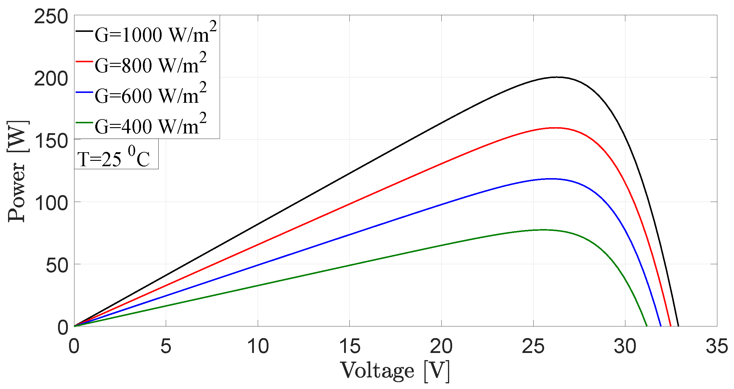
where is the generated photovoltaic current, n is the ideality (quality) constant of the diode, is the leakage current of the diode, is the equivalent series resistance, is the equivalent shunt resistance, is the number of series cells in the module, is the delivered current, and is the terminal output voltage. Based on that, the characteristics of the PV source (KC200GT) at various conditions are illustrated in Figure 1 and Figure 2 [14].
2.2. Boost Converter Modeling
The boost topology has two forms of operation according to the status of its power switch, which are the ON and OFF states. These states are clarified in Figure 3. Therefore, the performance of the boost converter is simply described as
where x = [ ] is the state vector, u = [ ] is the input vector, and is the output voltage. Additionally, , , , and are the system matrices and can be given as
where is the input voltage for the inverter, is inverter input current, L is the boost inductance, and are the capacitors at the PV source and inverter terminals, respectively, and d is the duty interval of the boost.
2.3. Model of the Inversion Stage with Grid Connection
The two-level inverter set-up with grid connection is shown in Figure 4. In fact, eight switching vectors can be produced from the two-level inverter. These switching patterns are also shown in Figure 4. Furthermore, the corresponding sector distribution is involved in the same figure [49].
In reference to Figure 4, one can simply obtain
where are the grid voltages, are the inverter output voltages, are the line currents, and and are the filter parameters.
In the stationary reference frame (-), Equation (4) is reformulated as
Furthermore, and in the (d-q) reference frame, the previous formula is written as
where is the grid-frequency. Then, the expressions of the active and reactive power at these frames are given by
3. Main Control Strategies for the Two-Stage PV System
3.1. Maximum Power Point Tracking
The objective of the MPPT algorithm is to pursue the maximum power from the PV source at different atmospheric conditions. In this regard, the most popular techniques and practically implemented in the industry are the P&O and INC [50]. The execution of both methods is simple, where no model dependency is required [17].
- The perturb and observe method
The working principle of this method depends on the P-V characteristics of the PV generator (Figure 1). Simply, the operating point is disturbed in one direction. For instance, the control parameter is increased and if the power grows, the perturbation is kept in the same direction (the control parameter will be increased again). Otherwise, the direction of the control parameter will be changed (reversed). Following this manner, the MPP will be reached after certain iterations [51,52]. This, in turn, implies oscillation around the MPP. To reduce this oscillation, the P&O method can be implemented by incorporating an adaptive step. In the present study, an adaptive step based on the slope of the PV power relative to the PV voltage is utilized as follows [36]
where is the present duty period, is the previous one, and N is a tuning factor. The idea behind this relation is that the slope of the P-V characteristics is large when the operating point is far from the MPP and small in the neighborhood of the MPP. Therefore, a big move is enforced when the system operation is far from the MPP. In contrast, a tiny step is provided as the system comes near the MPP, resulting in a lower ripple content in the PV power under steady-state operation. The tuning factor (N) is adjusted to regulate the step-size, which is the change of the duty cycle. Therefore, the value of the tuning factor specifies the performance of the MPPT algorithm. Figure 5 shows the algorithm of the P&O method with adaptive step realization.
- The incremental conductance method
It is known that the slope of the P-V curve at the left side of the MPP is positive and negative on the right part. Theoretically, the slope of the power with respect to the voltage equals zero at the MPP, and hence this can be mathematically formulated as [53]
where p, v, and i refer to the PV power, voltage, and current, respectively. Further manipulation can be performed to obtain the following:
where and represent the interval between two measurements. Simply, the basic concept of the INC method is stated in the following rule
In practice, it is hard to fulfill the condition in Equation (11). Therefore, a permitted error is allowed to achieve approximately zero oscillation around the MPP [34,54]. As a result, the mentioned formula is modified to
where e is the allowable value of error. It is worth indicating that if the power–current (P-I) characteristic is considered instead of the P-V curve, the method is recognized as the incremental resistance (INR) [55].
3.2. Active and Reactive Power Control
- The voltage-oriented control
The VOC is the most recognized method for active and reactive power regulation in grid-coupled applications. The primary principle of this technique is to align the grid voltage with the direct axis of the rotating reference frame (d-q) [40,56]. Therefore, the active and reactive power are decoupled, and hence, they can be controlled separately. In this case, Equation (8) is simplified to
Considering this, the active power can be directly managed by controlling the direct axis current (). By the same way, the reactive power is regulated using the quadrature axis current (). Normally, the direct axis current is drawn from the DC-link to achieve energy balance. Furthermore, the quadrature axis current is set to zero for unity power factor operation [40]. However, the quadrature axis current value can be adjusted to inject and support the system with reactive power, which in turn influences (reduces) the active power value to avoid overloading on the inverter [57]. To implement the VOC strategy, a cascaded loop structure is used employing PI controllers, where the outer loop provides the reference currents for the inner loop. Then, the reference voltage is computed and applied to the modulation stage.
- The finite-set model predictive control
FS-MPC has gotten a significant interest to control different power converters and machines. That is because the simple implementation, and the inclusion of additional control objectives and constraints [58]. The FS-MPC design is based on the discrete-time model of the system. In the case of the two-level inverter (the present utilized converter), Equation (4) can be discretized to
The FS-MPC principle implies calculating the previous predicted currents for all possible switching states of the utilized converter (8 for the two-level inverter). Following, the best state among them is chosen to be applied next in accordance with the cost function as follows
where and are the reference currents. Additional objectives can be added to the cost function. However, this comes at the cost of affecting the primary control objective. For example, if it is required to decrease the switching frequency as an additional objective, the cost function is modified to [49]
where is the present switching state, is the past one, and is a weighting factor. Hence, the switching frequency will be decreased based on the value of the weighting factor. This indeed affects the current tracking, resulting in an increased THD of the currents [46].
To decrease the computational burden of the FS-MPC, considering the current predictions and cost function evaluations (8 times for both), the reference voltage vector (RVV) is computed as follows [31,59]
Therefore, the cost function is calculated only for a definite number of voltage vectors, which are mainly in the neighborhood of the RVV. This can be implemented by sector identification or grouping of the converter switching vectors [31,46].
- The dead-beat technique
The DB is similar to the implementation of the FS-MPC. However, it has a fixed switching frequency due to the presence of a modulator. The idea behind this strategy is to force the predicted currents to be equal to the reference values at the next sampling instant [47]. This can be accomplished using the previously mentioned RVV in Equation (18) and a modulator. Furthermore, this technique (also the FS-MPC) can be directly implemented in the - reference frame, which implies modifying Equation (18) to
The control strategies are illustrated in Figure 6, where the VOC with two loop construction, the FS-MPC with the predictive principle, and the DB method are clarified.
3.3. Parameter Estimation Based on EKF
The predictive control techniques (including simplified algorithms) and the dead-beat method depend on the model of the system. Therefore, potential variation of the parameters of the system affects the performance of the controller [60]. Numerous methods have been investigated to address this issue, where different analytical methods and observers are implemented to account for the parameters change. Model reference adaptive system (MRAS) [61], Luenberger observe [62], extended Kalman filter [31], disturbance observer [63,64], and discrete-time integral action [64] have been discussed in the literature. EKF is an effective method to estimate the system’s parameters [31]. Its design is dependent on the discrete-time model of the structure. Therefore, it is chosen in this study to estimate the PV system parameters, which are the filter parameters namely the filter resistance and inductance. It should be mentioned that the authors presented EKF previously to address the problem of parameters variation with FS-MPC in [31]. However, only simulation results were provided in this study. Therefore, we are motivated to investigate that experimentally in this work.
To execute the EKF, the discrete-time model of the PV system is obtained by rearranging Equation (5) as
In fact, the model of the grid-integrated system incorporating disturbance is given by
where x = [ ] is the state vector, u = [( − ) ( − )] is the input states, y = [ ] is the measured values, w is the system uncertainty with covariance matrix , and v is the measurement noise with covariance matrix . Further, , , , and are the system matrices, which are defined according to Equation (20) as
Hence, the discrete model is given as
where , , , , and is the unity matrix. Normally, the variability (uncertainty) of the system and the noise related to the measurement are not identified; thus, the EKF is realized as
where is the Kalman costant, and and are the estimated values. At last, the EKF can be executed within two processes of prediction and correction according to the next steps:
- Initialization for the state variables and covariance matrices.
- Projection of state vector
- Prediction of error covariance matrixwhere
- Computation of Kalman constant
- Estimation correction based on measurements
- Update of error covariance matrix
- Repeat from step 2.
4. Experimental Tests and Evaluations
4.1. Lab Setup Description
The two-stage PV topology, which is considered for validation, consists of a PV emulator, DC-DC converter (boost), inverter, and R-L load. The emulator utilizes a DC source with a group of shunt resistors to emulate a step change in the PV power (radiation in real case) [46]. Measurement board is used to sense the voltages and currents required for implementation. As a real-time controller, dSPACE MicroLabBox is employed. The control techniques are built using Matlab platform and the results are captured with the assistance of control desk software. The test-bench configuration is shown in Figure 7, while the parameters of the arrangement are tabulated in Table 2.
4.2. Assessment of the MPPT Performance
The behavior of the MPPT using the adaptive P&O method is investigated in Figure 8. The results show the PV power, PV voltage, and PV current, respectively. The system operates under certain power level. Then, the PV power is increased in step manner and returned to its previous value. The P&O method succeeded to track the maximum power in different operating conditions with less oscillation at the steady-state. The adaptive step contributes to the limitation of the power ripple. The waveform of the duty cycle with adaptive step is further investigated in Figure 9, where the oscillation of the duty cycle is small. This, in turn, has a positive impact on the energy utilization. Therefore, the efficiency of the P&O technique is given in Table 3.
4.3. Inverter Control Results
In this subsection, the behavior of the VOC, FS-MPC, and DB techniques is discussed. Figure 10 shows the results of DC-link voltage, d-axis current, q-axis current, and the instantaneous currents, respectively. The behavior of the DC-link voltage is similar for all methods with moderate over and undershoots. The ripple content of d-axis current is small for the VOC method in comparison with the FS-MPC and DB. Furthermore, the oscillations of the d-axis current is the highest for the FS-MPC technique. The variable switching frequency behavior contributes to these high oscillations. It is worth mentioning that the average switching frequency at different operating conditions (for the FS-MPC) is comparable to the fixed switching frequency of the VOC and DB methods for fair comparison. Similarly, the q-axis current tracking is the best for the VOC method. However, the FS-MPC provides better q-axis current tracking when compared to the DB technique, especially at higher power values. Moreover, a small steady-state error can be observed between the d-axis current and its reference for the FS-MPC and DB. The reason for this steady-state deviation is the model parameter mismatches and the un-modeled dynamics of the system. As these approaches are more dependent on the model parameters when compared to the VOC technique.
The THD of the currents are summarized in Table 4, where the FS-MPC gives higher THD values due to the variable switching frequency nature. Furthermore, the THD values with the VOC are the lowest. The computational burden of all methods is further investigated in Table 5, where the execution times of all methods are provided. The FS-MPC requires a higher execution time in comparison with the VOC and DB due to the presence of the prediction stage and cost function computation for all switching states of the converter. However, the execution time of the DB is comparable to the VOC technique.
4.4. EKF Estimation
As raised earlier, the FS-MPC and DB rely on the system’s parameter. Therefore, to tackle this problem, the EKF is used to calculate these parameters. Figure 11 presents the estimation of the filter inductance and resistance at step change of the injected currents. The estimated values are in very good agreement with the nominal values (see Table 2), where the maximum error in inductance estimation is 4% and 1.8% in the resistance estimation.
Another merit of the EKF, which motivates the authors to employ it for parameters estimation, is the filtering capability of the EKF. This great advantage can provide a significant benefit in case of noisy measurements. Therefore, the estimated currents can be fed into the implemented control algorithm instead of the measured values. Figure 12 shows the actual and estimated currents in the - reference frame. Moreover, Table 6 gives the THD values of the actual and estimated currents. The THD values of the estimated (filtered) currents are greatly reduced when compared with the actual ones.
4.5. Robustness Assessment
In this part, the influence of the parameters change on the system will be investigated. The filter inductance is considered for analysis as the resistance effect is minor [31]. Two values are used to assess the effect of the inductance variation on the system, where one value represents a severe underestimation, and the other one is an overestimated value for the inductance. The chosen values are 7 and 15 mH, which represents 4 mH difference from the nominal value.
To have a clear picture of the inductance variation effect, the instantaneous currents are shown in Figure 13 for the two values of the inductance. Then, the THD values at inductance mismatch are calculated and tabulated in Table 7. From the table, the effect of inductance variation on the VOC is approximately negligible, where the THD values vary within a very narrow range. The FS-MPC and DB methods give better THD values at lower inductance values, which is normal due to the filtering behavior of the inductance [14]. The effect of inductance overestimation is more noticeable for the DB method in comparison with the FS-MPC, where, and at high inductance value, the THD increase in comparison with the nominal inductance (see Table 4 low power condition) is approximately 1% for the DB and 0.5% for the FS-MPC.
Even when the THD values get better with inductance underestimation, it should be mentioned that parameter mismatches affect the tracking behavior of the actual current with respect to its reference value. Figure 14 shows the response of the d-axis current at the previously mentioned inductance values. One can notice the steady-state error between the reference and actual currents.
To this end, Table 8 provides a comparative summary for the VOC, FS-MPC, and DB methods, where different aspects have been considered. The VOC gives the most adequate performance in steady-state and its computational burden is low. However, tuning effort for the PI controllers is considered a drawback of this method. The DB technique has also perfect steady-state behavior. However, the dependency on the parameters is high in this technique. The FS-MPC shows high ripple content at steady-state, but multi-objective handling is a big merit of this approach.
The VOC and DB methods are advised when fixed switching is preferred over the variable one. However, the VOC method has the advantage of fewer parameters dependency. On the other hand, the DB method allows simple implementation in comparison with VOC due to the low number of utilized PI controllers (at the outer loop only). FS-MPC is recommended in case of multi-objective requirements. It provides simple execution for the multi-task, which can be involved within the cost function design. Furthermore, it shows fast dynamics.
5. Future Work
The present study proposed a comparative study among the main control methods for grid integration of the PV system. The control objectives that have been discussed include the MPPT, adaptive implementation of MPPT, active and reactive power regulation, and robustness assessment and improvement. However, the authors believe that some key points should be addressed to further improve the research in the field of PV systems. To mention a few:
- Implementation of different power control strategies in addition to the MPPT function. The PV system should be able to support the grid [67]. In this matter, different functions are to be included within the MPPT operation. For example, constant power generation is required to protect the grid against overloading at situations of peak power generation [68].
- Simplification and calculation reduction of the FS-MPC techniques, especially when considering multilevel inverters [69].
- Multi-objective realization for the control scheme, where different purposes can be achieved.
- Sensorless control is preferred as a back-up strategy in situations of sensor failure, where the control objective can be fulfilled with a minimum number of sensors. However, this may lead to deterioration of the controller quality [72].
- Low voltage ride through capability and improvement of the PV system [73].
6. Conclusions
This article discusses the main control techniques of the two-stage PV system. Firstly, the P&O method is implemented for MPPT and an adaptive step is utilized to limit the steady-state oscillation in the PV power. Secondly, the inverter control strategies including the VOC, FS-MPC, and DB are discussed and compared together. The VOC and DB methods provide less steady-state oscillation in comparison with the FS-MPC. Furthermore, their switching frequency is fixed, which is preferred in some applications. The FS-MPC allows multi-task incorporation in the cost function design, which makes it an interesting option for multi-objectives. The DB and FS-MPC design depend on the parameters of the system. In this regard, the robustness of the DB is lower when compared to FS-MPC. Therefore, an EKF is utilized here for parameters estimation. Furthermore, the EKF provides filtering behavior. Thus, it can be advantageous in case of noisy measurements. Future research directions include multi-objective inclusion for the FS-MPC technique. Robustness enhancement for the DB method is also advised. For MPPT, the drift phenomenon at fast-changing atmospheric conditions is to be addressed and effectively solved.
Author Contributions
M.A. (Mostafa Ahmed) designed, implemented, the proposed control strategy, and wrote the manuscript. I.H. helped in writing the manuscript and collection of the experimental results. M.A. (Mohamed Abdelrahem) revised and edited the manuscript. R.K. and J.R. were responsible for guidance and suggestions. All authors have read and agreed to the published version of the manuscript.
Funding
This research received no external funding.
Institutional Review Board Statement
Not applicable.
Informed Consent Statement
Not applicable.
Data Availability Statement
Not applicable.
Acknowledgments
The work of José Rodríguez was supported by Agencia Nacional de Investigación y Desarrollo (ANID) under Project FB0008, Project 1210208, and Project 1221293.
Conflicts of Interest
The authors declare no conflict of interest.
References
- Alshahrani, A.; Omer, S.; Su, Y.; Mohamed, E.; Alotaibi, S. The technical challenges facing the integration of small-scale and large-scale PV systems into the grid: A critical review. Electronics 2019, 8, 1443. [Google Scholar] [CrossRef]
- Aleem, S.A.; Hussain, S.S.; Ustun, T.S. A review of strategies to increase PV penetration level in smart grids. Energies 2020, 13, 636. [Google Scholar] [CrossRef]
- Seyedmahmoudian, M.; Rahmani, R.; Mekhilef, S.; Oo, A.M.T.; Stojcevski, A.; Soon, T.K.; Ghandhari, A.S. Simulation and hardware implementation of new maximum power point tracking technique for partially shaded PV system using hybrid DEPSO method. IEEE Trans. Sustain. Energy 2015, 6, 850–862. [Google Scholar] [CrossRef]
- Liu, G.; Rasul, M.G.; Amanullah, M.T.O.; Khan, M.M.K. Techno-economic simulation and optimization of residential grid-connected PV system for the Queensland climate. Renew. Energy 2012, 45, 146–155. [Google Scholar] [CrossRef]
- Ahmed, J.; Salam, Z. A Maximum Power Point Tracking (MPPT) for PV system using Cuckoo Search with partial shading capability. Appl. Energy 2014, 119, 118–130. [Google Scholar] [CrossRef]
- Zheng, H.; Li, S.; Challoo, R.; Proano, J. Shading and bypass diode impacts to energy extraction of PV arrays under different converter configurations. Renew. Energy 2014, 68, 58–66. [Google Scholar] [CrossRef]
- Taghvaee, M.H.; Radzi, M.A.M.; Moosavain, S.M.; Hizam, H.; Marhaban, M.H. A current and future study on non-isolated DC–DC converters for photovoltaic applications. Renew. Sustain. Energy Rev. 2013, 17, 216–227. [Google Scholar] [CrossRef]
- Başoğlu, M.E. Comprehensive review on distributed maximum power point tracking: Submodule level and module level MPPT strategies. Sol. Energy 2022, 241, 85–108. [Google Scholar] [CrossRef]
- Ali, K.; Yasir, M.; Liu, H.; Yang, Z.; Yuan, X. A comprehensive review on grid connected photovoltaic inverters, their modulation techniques, and control strategies. Energies 2020, 13, 4185. [Google Scholar]
- Shawky, A.; Ahmed, M.; Orabi, M.; Aroudi, A.E. Classification of three-phase grid-tied microinverters in photovoltaic applications. Energies 2020, 13, 2929. [Google Scholar] [CrossRef]
- Wu, T.-F.; Chang, C.-H.; Lin, L.-C.; Kuo, C.-L. Power loss comparison of single-and two-stage grid-connected photovoltaic systems. IEEE Trans. Energy Convers. 2011, 26, 707–715. [Google Scholar] [CrossRef]
- Lakshmi, M.; Hemamalini, S. Coordinated control of MPPT and voltage regulation using single-stage high gain DC–DC converter in a grid-connected PV system. Electr. Power Syst. Res. 2019, 169, 65–73. [Google Scholar] [CrossRef]
- Kumar, N.; Singh, B.; Panigrahi, B.K. LLMLF-based control approach and LPO MPPT technique for improving performance of a multifunctional three-phase two-stage grid integrated PV system. IEEE Trans. Sustain. Energy 2019, 11, 371–380. [Google Scholar] [CrossRef]
- Ahmed, M.; Abdelrahem, M.; Harbi, I.; Kennel, R. An Adaptive Model-Based MPPT Technique with Drift-Avoidance for Grid-Connected PV Systems. Energies 2020, 13, 6656. [Google Scholar] [CrossRef]
- Karami, N.; Moubayed, N.; Outbib, R. General review and classification of different MPPT Techniques. Renew. Sustain. Energy Rev. 2017, 68, 1–18. [Google Scholar] [CrossRef]
- Motahhir, S.; Hammoumi, A.E.; Ghzizal, A.E. The most used MPPT algorithms: Review and the suitable low-cost embedded board for each algorithm. J. Clean. Prod. 2020, 246, 118983. [Google Scholar] [CrossRef]
- Sera, D.; Mathe, L.; Kerekes, T.; Spataru, S.V.; Teodorescu, R. On the perturb-and-observe and incremental conductance MPPT methods for PV systems. IEEE J. Photovolt. 2013, 3, 1070–1078. [Google Scholar] [CrossRef]
- Bhattacharyya, S.; Samanta, S.; Mishra, S. Steady Output and Fast Tracking MPPT (SOFT-MPPT) for P&O and InC Algorithms. IEEE Trans. Sustain. Energy 2020, 12, 293–302. [Google Scholar]
- Pradhan, R.; Subudhi, B. A steepest-descent based maximum power point tracking technique for a photovoltaic power system. In Proceedings of the 2012 2nd International Conference on Power, Control and Embedded Systems, Allahabad, India, 17–19 December 2012; IEEE: Piscataway, NJ, USA, 2012; pp. 1–6. [Google Scholar]
- Verma, D.; Nema, S.; Shandilya, A.M.; Dash, S.K. Maximum power point tracking (MPPT) techniques: Recapitulation in solar photovoltaic systems. Renew. Sustain. Energy Rev. 2016, 54, 1018–1034. [Google Scholar] [CrossRef]
- Sher, H.A.; Murtaza, A.F.; Noman, A.; Addoweesh, K.E.; Al-Haddad, K.; Chiaberge, M. A new sensorless hybrid MPPT algorithm based on fractional short-circuit current measurement and P&O MPPT. IEEE Trans. Sustain. Energy 2015, 6, 1426–1434. [Google Scholar]
- Nadeem, A.; Sher, H.A.; Murtaza, A.F. Online fractional open-circuit voltage maximum output power algorithm for photovoltaic modules. IET Renew. Power Gener. 2020, 14, 188–198. [Google Scholar] [CrossRef]
- Coelho, R.F.; Concer, F.M.; Martins, D.C. A MPPT approach based on temperature measurements applied in PV systems. In Proceedings of the 2010 IEEE International Conference on Sustainable Energy Technologies (ICSET), Kandy, Sri Lanka, 6–9 December 2010; IEEE: Piscataway, NJ, USA, 2010; pp. 1–6. [Google Scholar]
- De Brito, M.A.G.; Galotto, L.; Sampaio, L.P.; Melo, G.d.e.; Canesin, C.A. Evaluation of the main MPPT techniques for photovoltaic applications. IEEE Trans. Ind. Electron. 2012, 60, 1156–1167. [Google Scholar] [CrossRef]
- Li, X.; Wang, Q.; Wen, H.; Xiao, W. Comprehensive studies on operational principles for maximum power point tracking in photovoltaic systems. IEEE Access 2019, 7, 121407–121420. [Google Scholar] [CrossRef]
- Robles Algarín, C.; Giraldo, J.T.; Alvarez, O.R. Fuzzy logic based MPPT controller for a PV system. Energies 2017, 10, 2036. [Google Scholar] [CrossRef]
- Boumaaraf, H.; Talha, A.; Bouhali, O. A three-phase NPC grid-connected inverter for photovoltaic applications using neural network MPPT. Renew. Sustain. Energy Rev. 2015, 49, 1171–1179. [Google Scholar] [CrossRef]
- Messalti, S.; Harrag, A.; Loukriz, A. A new variable step size neural networks MPPT controller: Review, simulation and hardware implementation. Renew. Sustain. Energy Rev. 2017, 68, 221–233. [Google Scholar] [CrossRef]
- Podder, A.K.; Roy, N.K.; Pota, H.R. MPPT methods for solar PV systems: A critical review based on tracking nature. IET Renew. Power Gener. 2019, 13, 1615–1632. [Google Scholar] [CrossRef]
- Mohanty, S.; Subudhi, B.; Ray, P.K. A new MPPT design using grey wolf optimization technique for photovoltaic system under partial shading conditions. IEEE Trans. Sustain. Energy 2015, 7, 181–188. [Google Scholar] [CrossRef]
- Ahmed, M.; Abdelrahem, M.; Kennel, R. Highly efficient and robust grid connected photovoltaic system based model predictive control with kalman filtering capability. Sustainability 2020, 12, 4542. [Google Scholar] [CrossRef]
- Kermadi, M.; Salam, Z.; Eltamaly, A.M.; Ahmed, J.; Mekhilef, S.; Larbes, C.; Berkouk, E.M. Recent developments of MPPT techniques for PV systems under partial shading conditions: A critical review and performance evaluation. IET Renew. Power Gener. 2020, 14, 3401–3417. [Google Scholar] [CrossRef]
- Seyedmahmoudian, M.; Horan, B.; Soon, T.K.; Rahmani, R.; Oo, A.M.T.; Mekhilef, S.; Stojcevski, A. State of the art artificial intelligence-based MPPT techniques for mitigating partial shading effects on PV systems—A review. Renew. Sustain. Energy Rev. 2016, 64, 435–455. [Google Scholar] [CrossRef]
- Safari, A.; Mekhilef, S. Simulation and hardware implementation of incremental conductance MPPT with direct control method using cuk converter. IEEE Trans. Ind. Electron. 2010, 58, 1154–1161. [Google Scholar] [CrossRef]
- Elgendy, M.A.; Zahawi, B.; Atkinson, D.J. Assessment of perturb and observe MPPT algorithm implementation techniques for PV pumping applications. IEEE Trans. Sustain. Energy 2011, 3, 21–33. [Google Scholar] [CrossRef]
- Liu, F.; Duan, S.; Liu, F.; Liu, B.; Kang, Y. A variable step size INC MPPT method for PV systems. IEEE Trans. Ind. Electron. 2008, 55, 622–2628. [Google Scholar]
- Loukriz, A.; Haddadi, M.; Messalti, S. Simulation and experimental design of a new advanced variable step size Incremental Conductance MPPT algorithm for PV systems. ISA Trans. 2016, 62, 30–38. [Google Scholar] [CrossRef] [PubMed]
- Zhang, F.; Thanapalan, K.; Procter, A.; Carr, S.; Maddy, J. Adaptive hybrid maximum power point tracking method for a photovoltaic system. IEEE Trans. Energy Convers. 2013, 28, 353–360. [Google Scholar] [CrossRef]
- Zakzouk, N.E.; Elsaharty, M.A.; Abdelsalam, A.K.; Helal, A.A.; Williams, B.W. Improved performance low-cost incremental conductance PV MPPT technique. IET Renew. Power Gener. 2016, 10, 561–574. [Google Scholar] [CrossRef]
- Kadri, R.; Gaubert, J.-P.; Champenois, G. An improved maximum power point tracking for photovoltaic grid-connected inverter based on voltage-oriented control. IEEE Trans. Ind. Electron. 2010, 58, 66–75. [Google Scholar] [CrossRef]
- Noguchi, T.; Tomiki, H.; Kondo, S.; Takahashi, I. Direct power control of PWM converter without power-source voltage sensors. IEEE Trans. Ind. Appl. 1998, 34, 473–479. [Google Scholar] [CrossRef]
- Zhang, N.; Tang, H.; Yao, C. A systematic method for designing a PR controller and active damping of the LCL filter for single-phase grid-connected PV inverters. Energies 2014, 7, 3934–3954. [Google Scholar] [CrossRef]
- Tafti, H.D.; Maswood, A.I.; Ukil, A.; Gabriel, O.H.P.; Ziyou, L. NPC photovoltaic grid-connected inverter using proportional-resonant controller. In Proceedings of the 2014 IEEE PES Asia-Pacific Power and Energy Engineering Conference (APPEEC), Hong Kong, China, 7–10 December 2014; IEEE: Piscataway, NJ, USA, 2014; pp. 1–6. [Google Scholar]
- Rodriguez, J.; Garcia, C.; Mora, A.; Flores-Bahamonde, F.; Acuna, P.; Novak, M.; Zhang, Y.; Tarisciotti, L.; Davari, S.A.; Zhang, Z.; et al. Latest advances of model predictive control in electrical drives. Part I: Basic concepts and advanced strategies. IEEE Trans. Power Electron. 2021, 37, 3927–3942. [Google Scholar] [CrossRef]
- Wang, F.; Zhang, Z.; Mei, X.; Rodríguez, J.; Kennel, R. Advanced control strategies of induction machine: Field oriented control, direct torque control and model predictive control. Energies 2018, 11, 120. [Google Scholar] [CrossRef]
- Ahmed, M.; Harbi, I.; Kennel, R.; Abdelrahem, M. Predictive Fixed Switching Maximum Power Point Tracking Algorithm with Dual Adaptive Step-Size for PV Systems. Electronics 2021, 10, 3109. [Google Scholar] [CrossRef]
- Bouafia, A.; Gaubert, J.-P.; Krim, F. Predictive direct power control of three-phase pulsewidth modulation (PWM) rectifier using space-vector modulation (SVM). IEEE Trans. Power Electron. 2009, 25, 228–236. [Google Scholar] [CrossRef]
- Shongwe, S.; Hanif, M. Comparative analysis of different single-diode PV modeling methods. IEEE J. Photovolt. 2015, 5, 938–946. [Google Scholar] [CrossRef]
- Rodriguez, J.; Cortes, P. Predictive Control of Power Converters and Electrical Drives; John Wiley & Sons: Hoboken, NJ, USA, 2012; Volume 40. [Google Scholar]
- Manoharan, P.; Subramaniam, U.; Babu, T.S.; Padmanaban, S.; Holm-Nielsen, J.B.; Mitolo, M.; Ravichandran, S. Improved perturb and observation maximum power point tracking technique for solar photovoltaic power generation systems. IEEE Syst. J. 2020, 15, 3024–3035. [Google Scholar] [CrossRef]
- Abdelsalam, A.K.; Massoud, A.M.; Ahmed, S.; Enjeti, P.N. High-performance adaptive perturb and observe MPPT technique for photovoltaic-based microgrids. IEEE Trans. Power Electron. 2011, 26, 1010–1021. [Google Scholar] [CrossRef]
- Killi, M.; Samanta, S. Modified perturb and observe MPPT algorithm for drift avoidance in photovoltaic systems. IEEE Trans. Ind. Electron. 2015, 62, 5549–5559. [Google Scholar] [CrossRef]
- Ishaque, K.; Salam, Z. A review of maximum power point tracking techniques of PV system for uniform insolation and partial shading condition. Renew. Sustain. Energy Rev. 2013, 19, 475–488. [Google Scholar] [CrossRef]
- Soon, T.K.; Mekhilef, S. A fast-converging MPPT technique for photovoltaic system under fast-varying solar irradiation and load resistance. IEEE Trans. Ind. Inform. 2014, 11, 176–186. [Google Scholar] [CrossRef]
- Mei, Q.; Shan, M.; Liu, L.; Guerrero, J.M. A novel improved variable step-size incremental-resistance MPPT method for PV systems. IEEE Trans. Ind. Electron. 2010, 58, 2427–2434. [Google Scholar] [CrossRef]
- Blaabjerg, F.; Teodorescu, R.; Liserre, M.; Timbus, A.V. Overview of control and grid synchronization for distributed power generation systems. IEEE Trans. Ind. Electron. 2006, 53, 1398–1409. [Google Scholar] [CrossRef]
- Yang, Y.; Wang, H.; Blaabjerg, F. Reactive power injection strategies for single-phase photovoltaic systems considering grid requirements. IEEE Trans. Ind. Appl. 2014, 50, 4065–4076. [Google Scholar] [CrossRef]
- Rodríguez, J.; Kennel, R.M.; Espinoza, J.R.; Trincado, M.; Silva, C.A.; Rojas, C.A. High-performance control strategies for electrical drives: An experimental assessment. IEEE Trans. Ind. Electron. 2011, 59, 812–820. [Google Scholar] [CrossRef]
- Xia, C.; Liu, T.; Shi, T.; Song, Z. A simplified finite-control-set model-predictive control for power converters. IEEE Trans. Ind. Inform. 2013, 10, 991–1002. [Google Scholar]
- Young, H.A.; Perez, M.A.; Rodriguez, J. Analysis of finite-control-set model predictive current control with model parameter mismatch in a three-phase inverter. IEEE Trans. Ind. Electron. 2016, 63, 3100–3107. [Google Scholar] [CrossRef]
- Liu, X.; Wang, D.; Peng, Z. Improved finite-control-set model predictive control for active front-end rectifiers with simplified computational approach and on-line parameter identification. ISA Trans. 2017, 69, 51–64. [Google Scholar] [CrossRef]
- Yan, L.; Song, X. Design and implementation of Luenberger model-based predictive torque control of induction machine for robustness improvement. IEEE Trans. Power Electron. 2019, 35, 2257–2262. [Google Scholar] [CrossRef]
- Yang, H.; Zhang, Y.; Liang, J.; Liu, J.; Zhang, N.; Walker, P.D. Robust deadbeat predictive power control with a discrete-time disturbance observer for PWM rectifiers under unbalanced grid conditions. IEEE Trans. Power Electron. 2018, 34, 287–300. [Google Scholar] [CrossRef]
- Abdelrahem, M.; Hackl, C.M.; Kennel, R.; Rodriguez, J. Efficient direct-model predictive control with discrete-time integral action for PMSGs. IEEE Trans. Energy Convers. 2018, 34, 1063–1072. [Google Scholar] [CrossRef]
- Eltamaly, A.M. A novel musical chairs algorithm applied for MPPT of PV systems. Renew. Sustain. Energy Rev. 2021, 146, 111135. [Google Scholar] [CrossRef]
- Ahmed, J.; Salam, Z. A modified P&O maximum power point tracking method with reduced steady-state oscillation and improved tracking efficiency. IEEE Trans. Sustain. Energy 2016, 7, 1506–1515. [Google Scholar]
- Tafti, H.D.; Konstantinou, G.; Townsend, C.D.; Farivar, G.G.; Sangwongwanich, A.; Yang, Y.; Pou, J.; Blaabjerg, F. Extended functionalities of photovoltaic systems with flexible power point tracking: Recent advances. IEEE Trans. Power Electron. 2020, 35, 9342–9356. [Google Scholar] [CrossRef]
- Peng, Q.; Sangwongwanich, A.; Yang, Y.; Blaabjerg, F. Grid-friendly power control for smart photovoltaic systems. Sol. Energy 2020, 210, 115–127. [Google Scholar] [CrossRef]
- Novak, M.; Dragicevic, T. Supervised Imitation Learn. Finite-Set Model Predict. Control Syst. Power Electronics. IEEE Trans. Ind. Electron. 2020, 68, 1717–1723. [Google Scholar] [CrossRef]
- Dragičević, T.; Novak, M. Weighting factor design in model predictive control of power electronic converters: An artificial neural network approach. IEEE Trans. Ind. Electron. 2018, 66, 8870–8880. [Google Scholar] [CrossRef] [Green Version]
- Elmorshedy, M.F.; Xu, W.; Allam, S.M.; Rodriguez, J.; Garcia, C. MTPA-based finite-set model predictive control without weighting factors for linear induction machine. IEEE Trans. Ind. Electron. 2020, 68, 2034–2047. [Google Scholar] [CrossRef]
- Chen, X.; Wu, W.; Gao, N.; Chung, H.S.-H.; Liserre, M.; Blaabjerg, F. Finite control set model predictive control for LCL-filtered grid-tied inverter with minimum sensors. IEEE Trans. Ind. Electron. 2020, 67, 9980–9990. [Google Scholar] [CrossRef]
- Al-Shetwi, A.Q.; Sujod, M.Z.; Blaabjerg, F. Low voltage ride-through capability control for single-stage inverter-based grid-connected photovoltaic power plant. Sol. Energy 2018, 159, 665–681. [Google Scholar] [CrossRef] [Green Version]
Figure 1.
P-V characteristics of the PV source at various irradiance conditions.

Figure 2.
I-V characteristics of the PV source at various irradiance conditions.

Figure 3.
Structure of the boost converter when: (a) Switch is OFF, and (b) switch is ON.

Figure 4.
(a) Two-level inverter configuration with grid coupling. (b) Switching actions and voltage vectors of the two-level inverter.
Figure 4.
(a) Two-level inverter configuration with grid coupling. (b) Switching actions and voltage vectors of the two-level inverter.

Figure 5.
The algorithm of the P&O method using adaptive step operation.

Figure 6.
Active and reactive power regulation methods for grid-tied PV systems (a) The VOC technique. (b) The FS-MPC approach. (c) The DB function.
Figure 6.
Active and reactive power regulation methods for grid-tied PV systems (a) The VOC technique. (b) The FS-MPC approach. (c) The DB function.

Figure 7.
The laboratory setup of the two-stage PV system.

Figure 8.
The performance of the P&O algorithm with adaptive process.

Figure 9.
Duty cycle variation under adaptive step operation.

Figure 10.
The behavior of the inverter control techniques at step change of the PV power: (a) The VOC method. (b) The FS-MPC technique. (c) The DB approach.
Figure 10.
The behavior of the inverter control techniques at step change of the PV power: (a) The VOC method. (b) The FS-MPC technique. (c) The DB approach.

Figure 11.
The estimated parameters at step change of the current: (a) Filter inductance. (b) Filter resistance.
Figure 11.
The estimated parameters at step change of the current: (a) Filter inductance. (b) Filter resistance.

Figure 12.
The current values in - reference frame. (a) Actual currents. (b) Estimated quantities.

Figure 13.
The currents at inductance variation where (1) is the underestimated inductance and (2) is the overestimated one: (a) The VOC method; (b) The FS-MPC technique; (c) The DB approach.
Figure 13.
The currents at inductance variation where (1) is the underestimated inductance and (2) is the overestimated one: (a) The VOC method; (b) The FS-MPC technique; (c) The DB approach.

Figure 14.
The d-axis currents at inductance variation where (1) is the underestimated inductance and (2) is the overestimated one: (a) The VOC method; (b) The FS-MPC technique; (c) The DB approach.
Figure 14.
The d-axis currents at inductance variation where (1) is the underestimated inductance and (2) is the overestimated one: (a) The VOC method; (b) The FS-MPC technique; (c) The DB approach.


Table 2.
PV system variables.
| Variable | Value |
|---|---|
| Boost inductance | mH |
| DC-link capacitor | |
| Power switch | single switch (IGBT-Module FF50R12RT4) |
| Diode | fast recovery diode BYW77PI200 |
| DC-link reference voltage | 50 V |
| Load resistance | |
| Load inductance | 11 mH |
| PV emulator resistors | / |
| Sampling time |
Table 3.
Average efficiency of the P&O technique.
| Method | (%) |
|---|---|
| P&O with adaptive step-size | 97.45 |
Table 4.
THD values of the currents for the VOC, FS-MPC, and DB techniques.
| Technique | THD % |
|---|---|
| VOC (low/high power) | 3.59/ 2.48 |
| FS-MPC (low/high power) | 4.52/ 3.41 |
| DB (low/high power) | 3.80/ 3.01 |
Table 5.
Execution times of the inverter control techniques.
| Method | Execution Time (s) |
|---|---|
| VOC | 14.62 |
| FS-MPC | 15.22 |
| DB | 14.51 |
Table 6.
THD values of the actual and filtered currents.
| Case | THD % |
|---|---|
| Actual (low/high power) | 3.81/3.05 |
| Filtered (low/high power) | 1.55/1.97 |
Table 7.
THD values at under- and overestimated filter inductance.
| Method | THD % (7 mH/15 mH) |
|---|---|
| VOC | 3.59/3.61 |
| FS-MPC | 4.42/4.99 |
| DB | 3.61/4.89 |
Table 8.
Comparative summary for the inverter control methods.
| Parameter | VOC | FS-MPC | DB |
|---|---|---|---|
| Switching frequency | Fixed | Variable | Fixed |
| PI requirements | 3 | 1 | 1 |
| Computation burden | Low | Moderate | Low |
| Steady-state performance | Excellent | Good | Very good |
| Tuning efforts | High | Low | Low |
| Dependency on parameters | Low | Moderate | High |
| Multi-objective inclusion | Hard | Easy | Hard |
Publisher’s Note: MDPI stays neutral with regard to jurisdictional claims in published maps and institutional affiliations. |
© 2022 by the authors. Licensee MDPI, Basel, Switzerland. This article is an open access article distributed under the terms and conditions of the Creative Commons Attribution (CC BY) license (https://creativecommons.org/licenses/by/4.0/).
Share and Cite
MDPI and ACS Style
Ahmed, M.; Harbi, I.; Kennel, R.; Rodríguez, J.; Abdelrahem, M. Evaluation of the Main Control Strategies for Grid-Connected PV Systems. Sustainability 2022, 14, 11142. https://doi.org/10.3390/su141811142
AMA Style
Ahmed M, Harbi I, Kennel R, Rodríguez J, Abdelrahem M. Evaluation of the Main Control Strategies for Grid-Connected PV Systems. Sustainability. 2022; 14(18):11142. https://doi.org/10.3390/su141811142
Chicago/Turabian StyleAhmed, Mostafa, Ibrahim Harbi, Ralph Kennel, José Rodríguez, and Mohamed Abdelrahem. 2022. "Evaluation of the Main Control Strategies for Grid-Connected PV Systems" Sustainability 14, no. 18: 11142. https://doi.org/10.3390/su141811142
Note that from the first issue of 2016, this journal uses article numbers instead of page numbers. See further details here.