
Modeling to Factor Productivity of the United Kingdom Food Chain: Using a New Lifetime-Generated Family of Distributions

 ,
,  and
and 
Abstract
:1. Introduction
- The first dataset: It represents the food chain in the United Kingdom from 2000 to 2019. The food sector plays a significant part in our economy, accounting for about 9 per cent of the Gross Value Added of the UK non-financial business economy. Four sectors make up the food chain: manufacture, wholesale, retail and non-residential catering. Both alcoholic and non-alcoholic drinks are included in food. Total factor productivity is a measure of the efficiency with which inputs are converted into outputs. For example, TFP increases if the volume of outputs increases while the volume of inputs stays the same. Similarly, TFP increases if the volume of inputs decreases while the volume of outputs stays the same. Although there is a practical limit on how much food people want to buy, the volume of output can increase due to increases in quality of products and by increases in exports.
- The second dataset: It represents the food and drink wholesaling in the United Kingdom from 2000 to 2019 as one factor of FTP.
- The third dataset: It is called the Single carbon fiber data and it is contains the tensile strength of single carbon fibers (in GPa).
- The fourth dataset: It is often called the breaking stress of carbon fibers dataset.
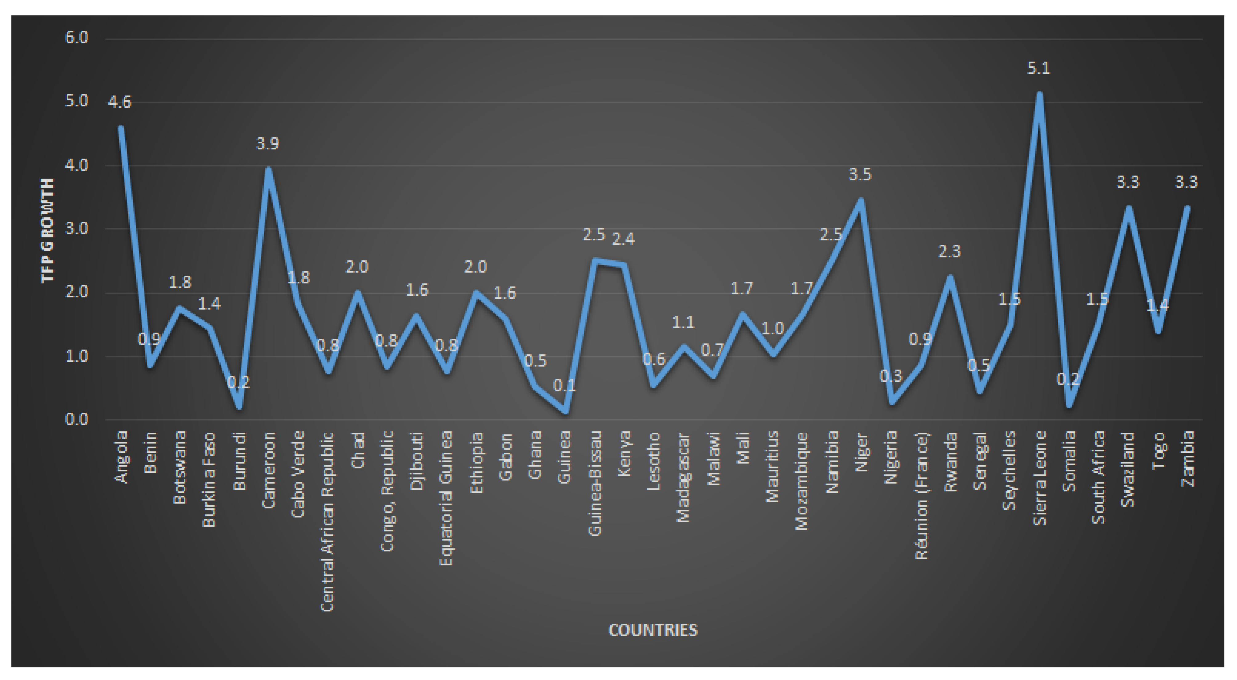
- The fifth dataset: It represents the TFP growth agricultural production for thirty-seven African countries from 2001–2010 as reported in Figure 1. Increasing the efficiency of agricultural production—getting more output from the same amount of resources—is critical for improving food security. To measure the efficiency of agricultural systems, we use TFP. TFP is an indicator of how efficiently agricultural land, labor, capital, and materials (agricultural inputs) are used to produce a country’s crops and livestock (agricultural output)—it is calculated as the ratio of total agricultural output to total production inputs. When more output is produced from a constant amount of resources, meaning that resources are being used more efficiently, TFP increases. Measures of land and labor productivity—partial factor productivity (PFP) measures—are calculated as the ratio of total output to total agricultural area (land productivity) and to the number of economically active persons in agriculture (labor productivity). Because PFP measures are easy to estimate, they are often used to measure agricultural production performance. These measures normally show higher rates of growth than TFP because growth in land and labor productivity can result not only from increases in TFP but also from a more intensive use of other inputs (such as fertilizer or machinery). Indicators of both TFP and PFP contribute to the understanding of agricultural systems needed for policy and investment decisions by enabling comparisons across time and across countries and regions. These TFP and PFP estimates were generated using the most recent data from Economic Research Service of the United States Department of Agriculture (ERS-USDA), the FAOSTAT database of the Food and Agriculture Organization of the United Nations (FAO), and national statistical sources.
2. The Sine-Exponentiated Weibull-H Family
3. Linear Representations
4. Some Special Models of the SEW-H Family
5. Statistical Properties
5.1. Quantile Function
5.2. Various Types of Moments
5.3. Order Statistics
6. Estimation Methods
6.1. Maximum Likelihood Estimation
6.2. Weighted and Ordinary Least Square
6.3. Product Spacing’s Method
6.4. Cramér–von-Mises
6.5. Anderson–Darling Method
7. Simulation
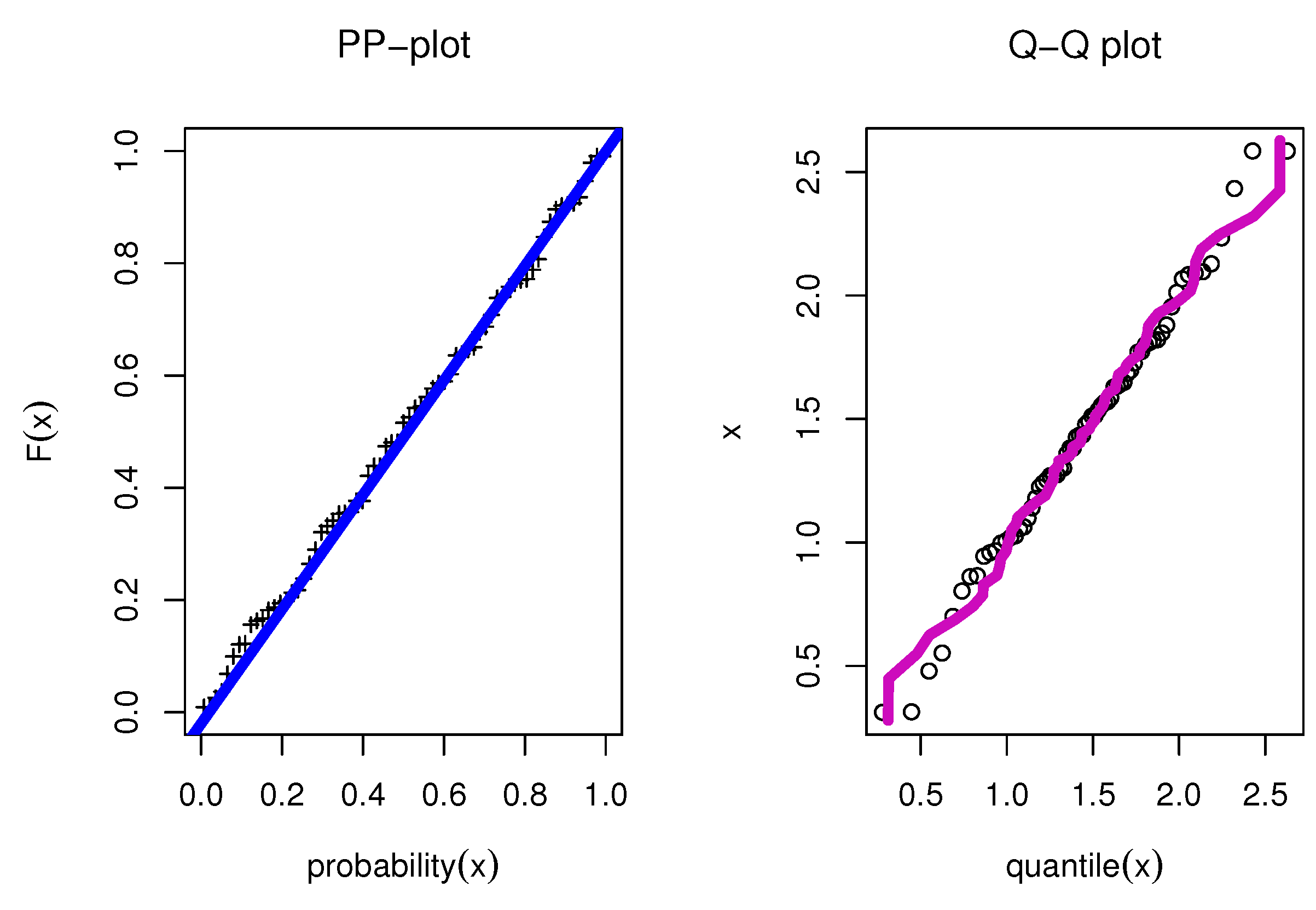
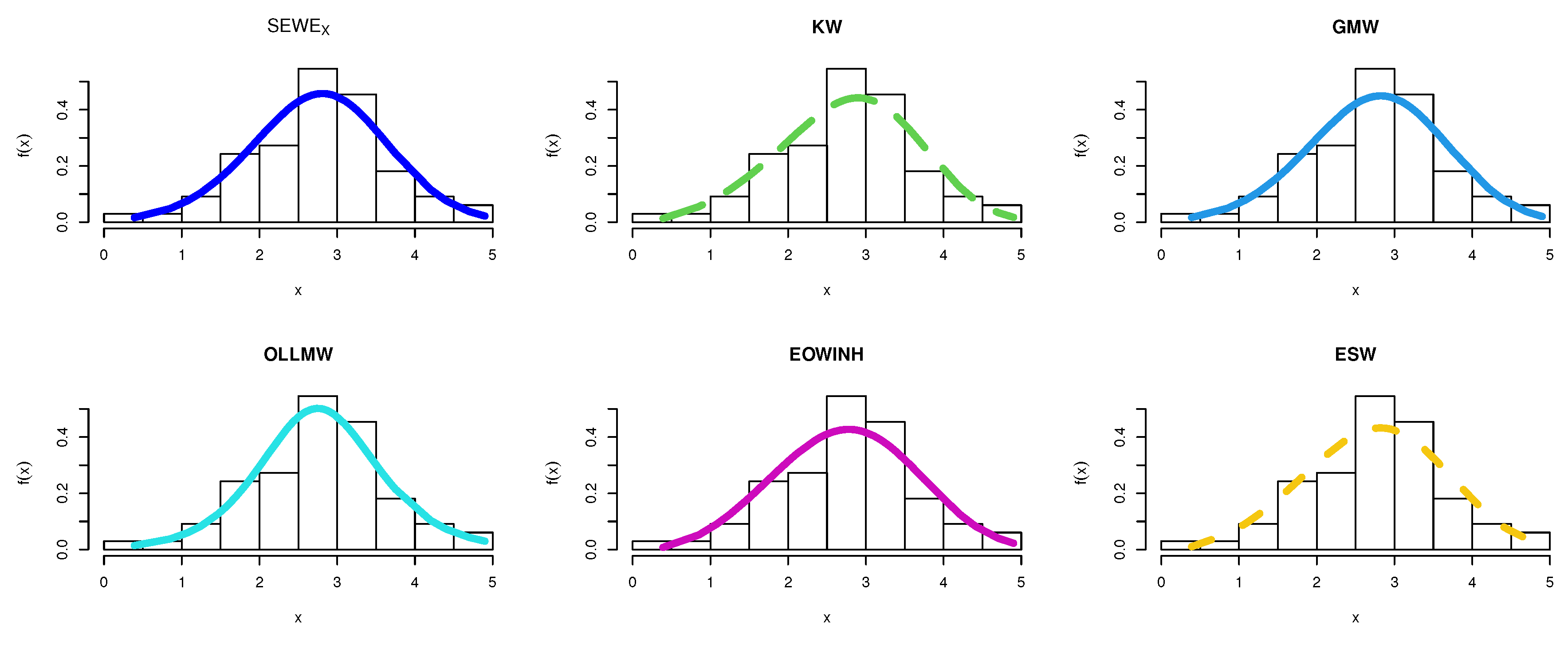
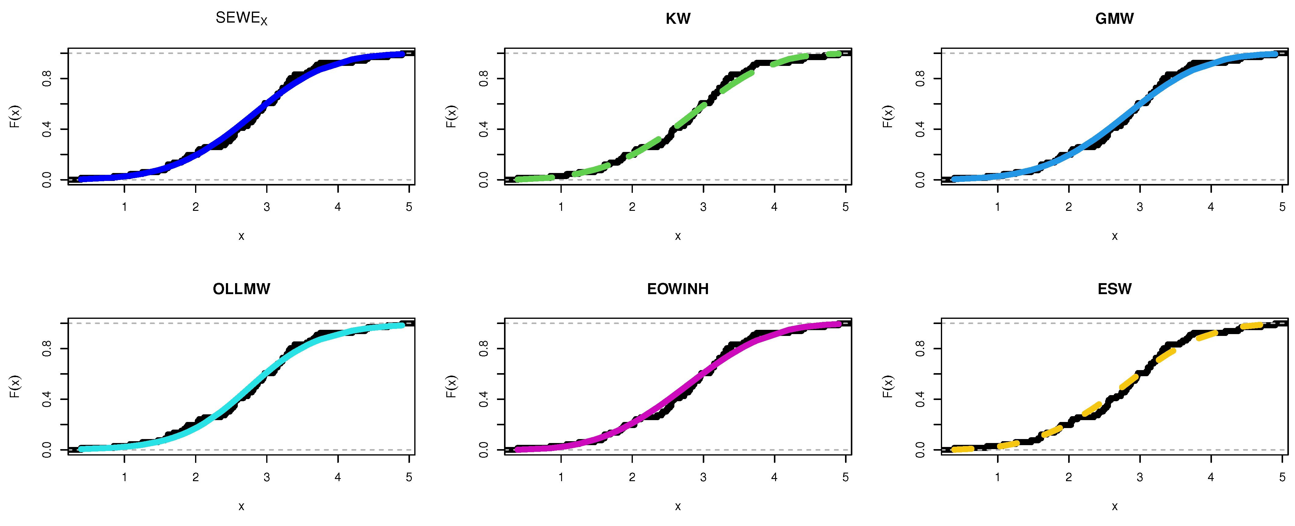
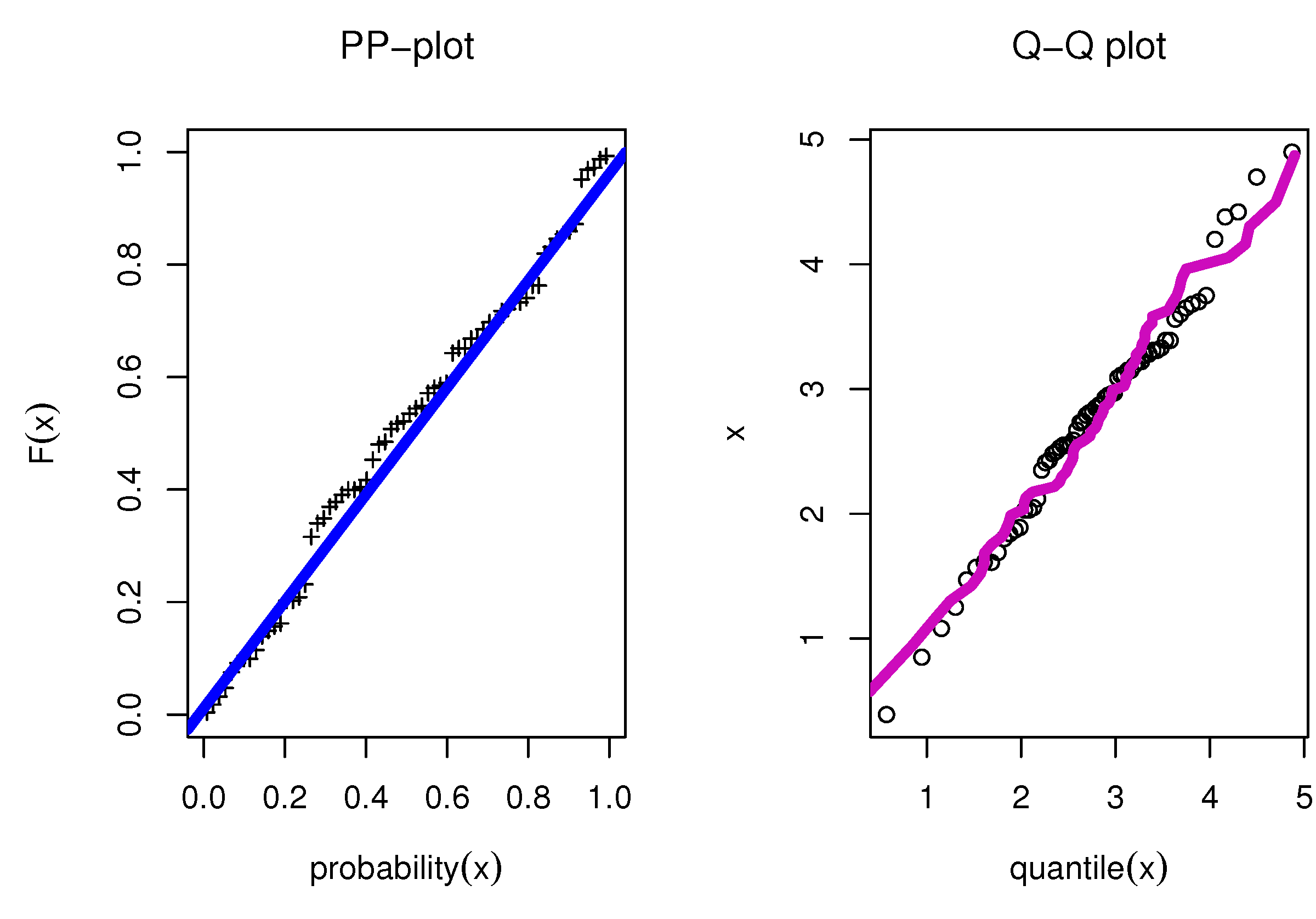
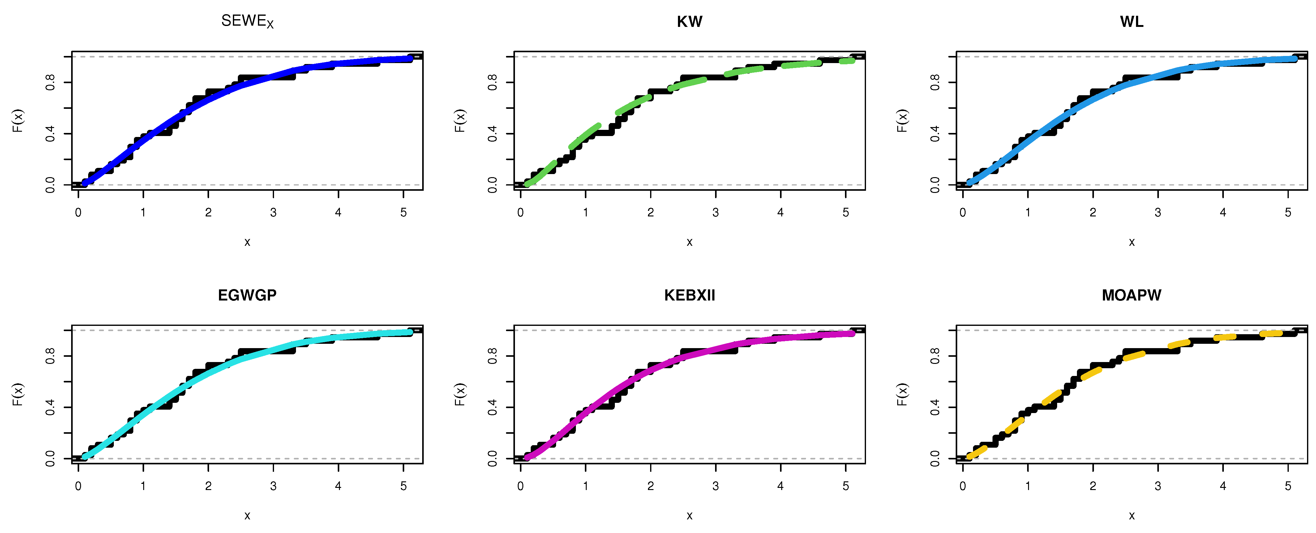
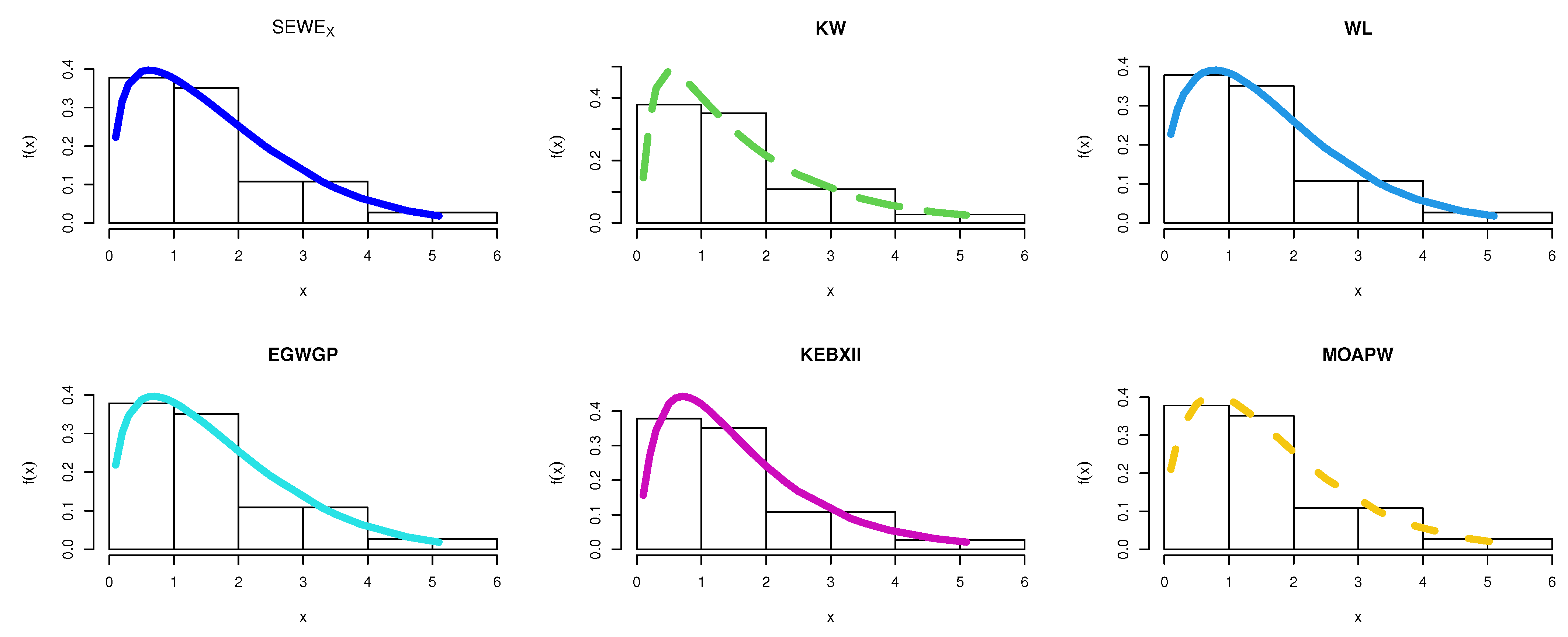
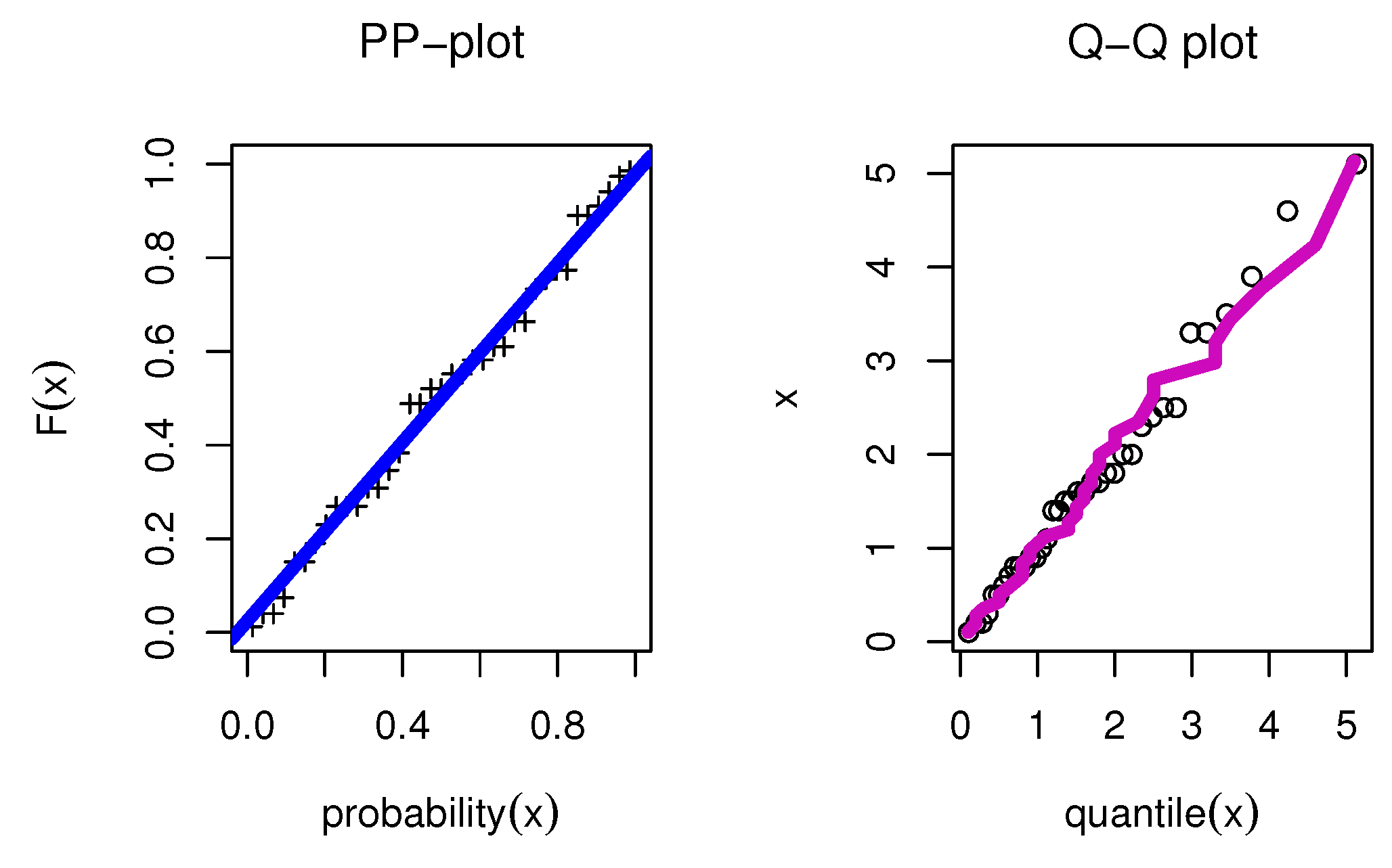
8. Applications
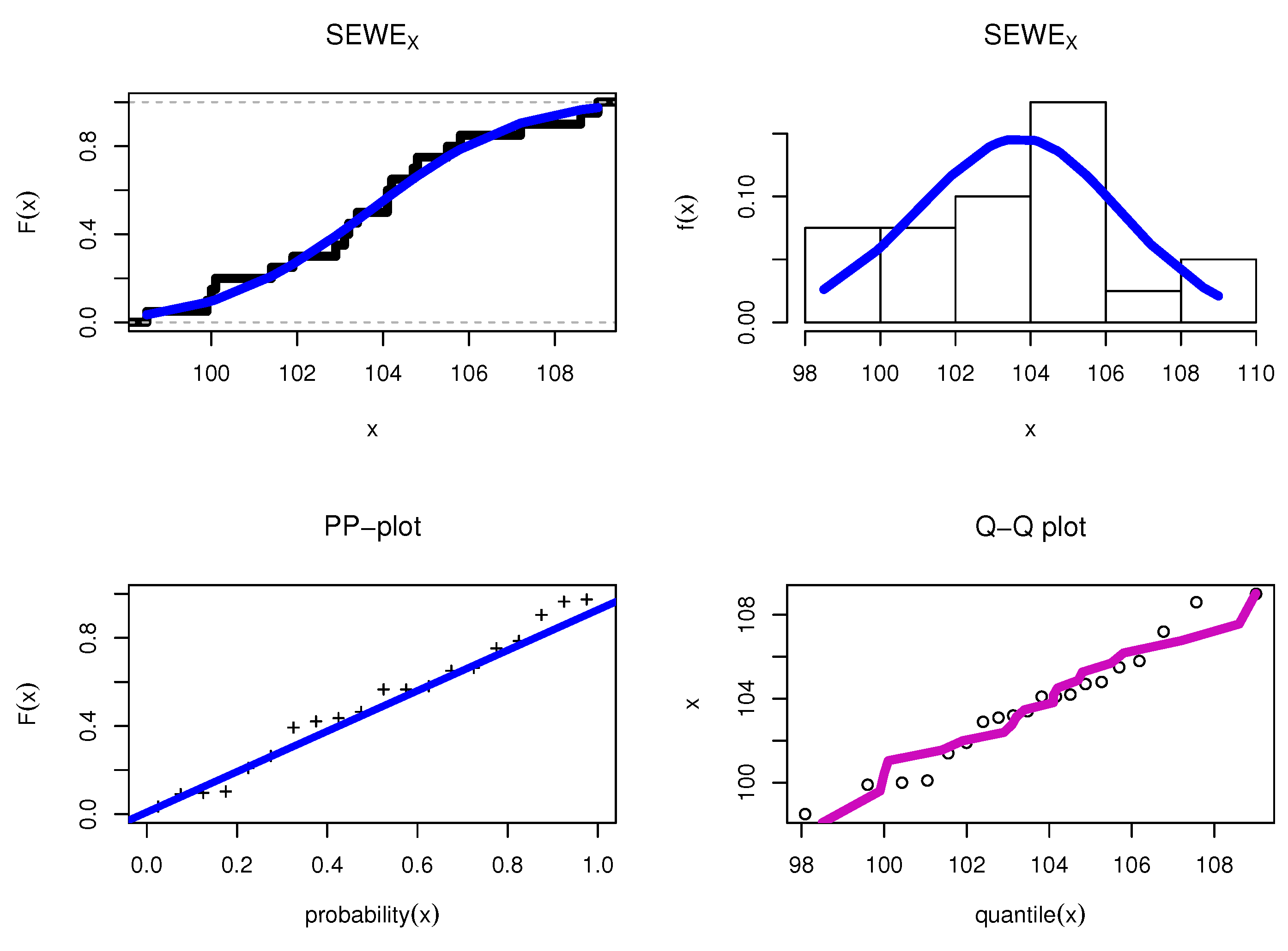
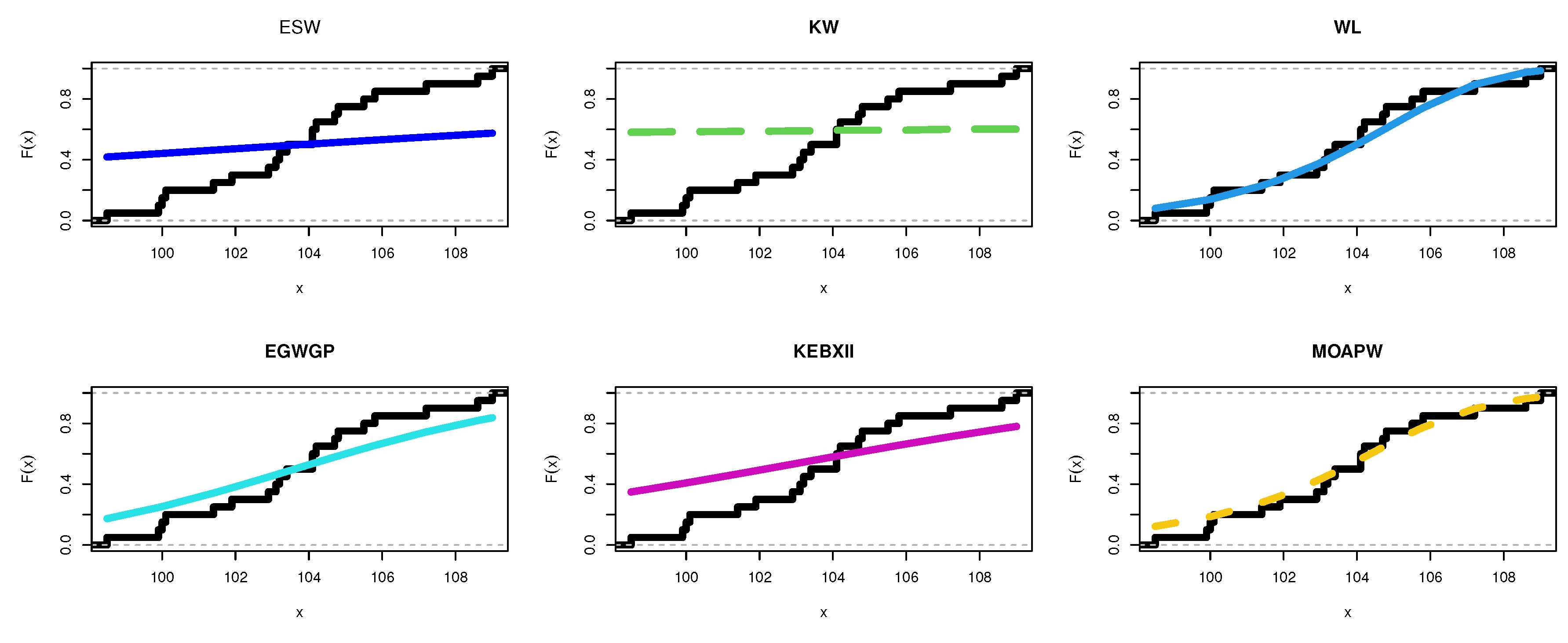
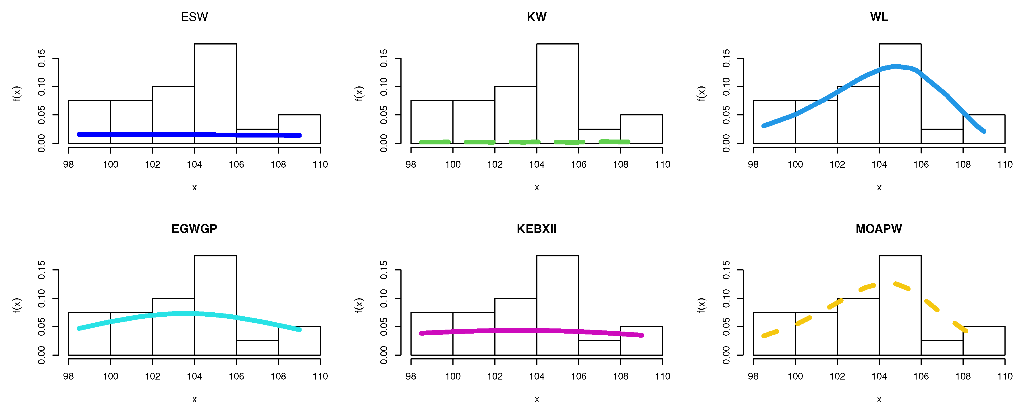
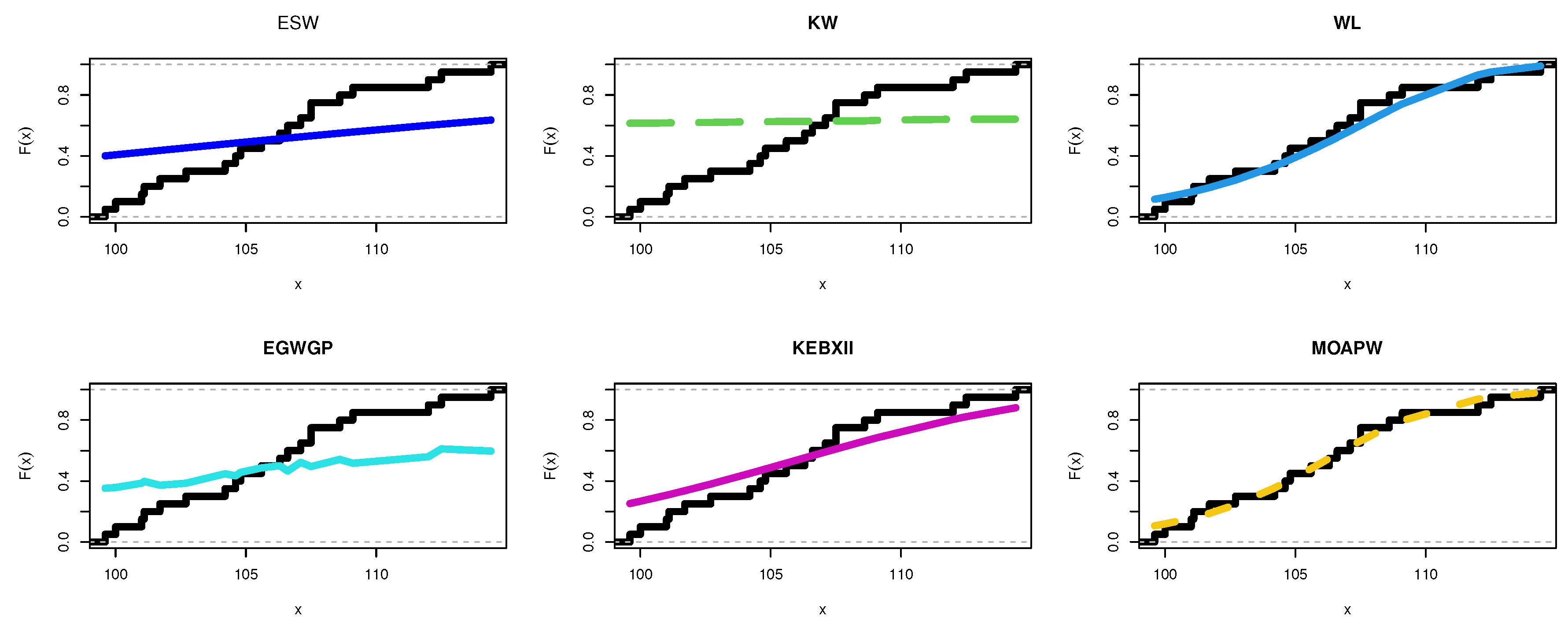
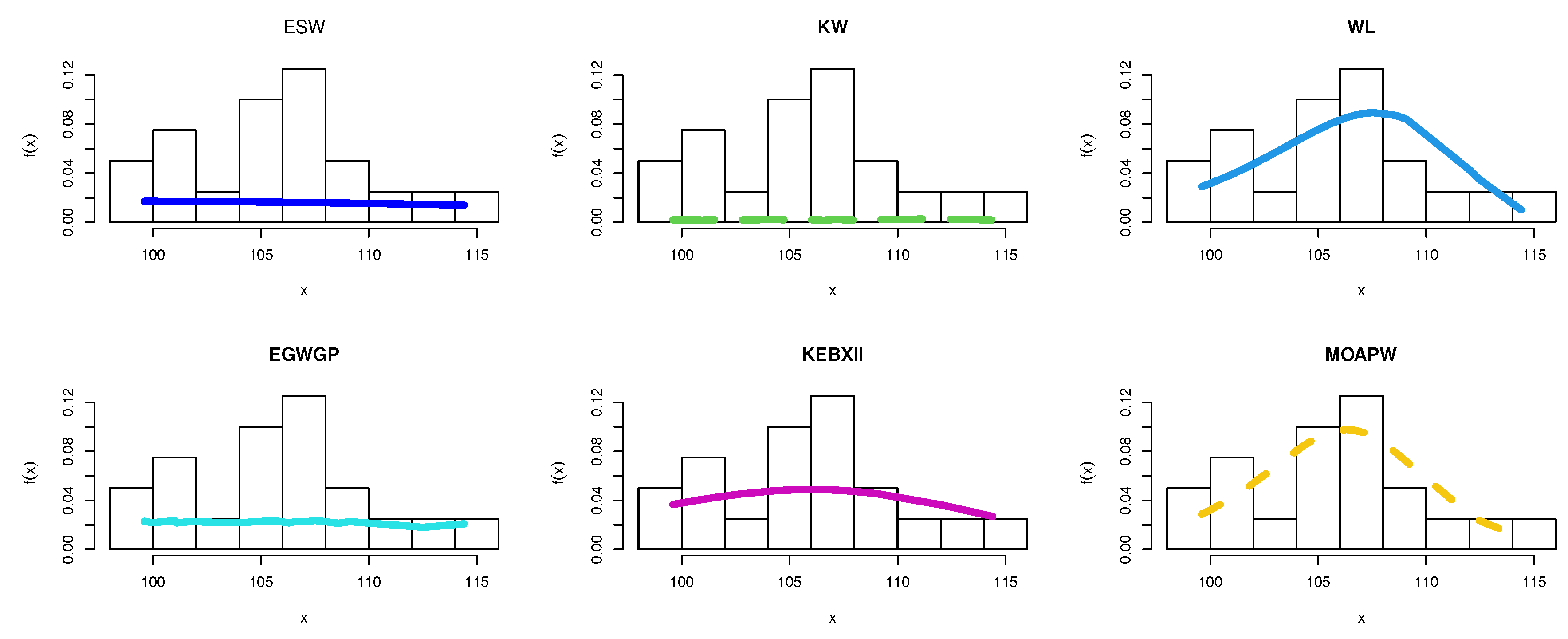
8.1. Food Chain Data
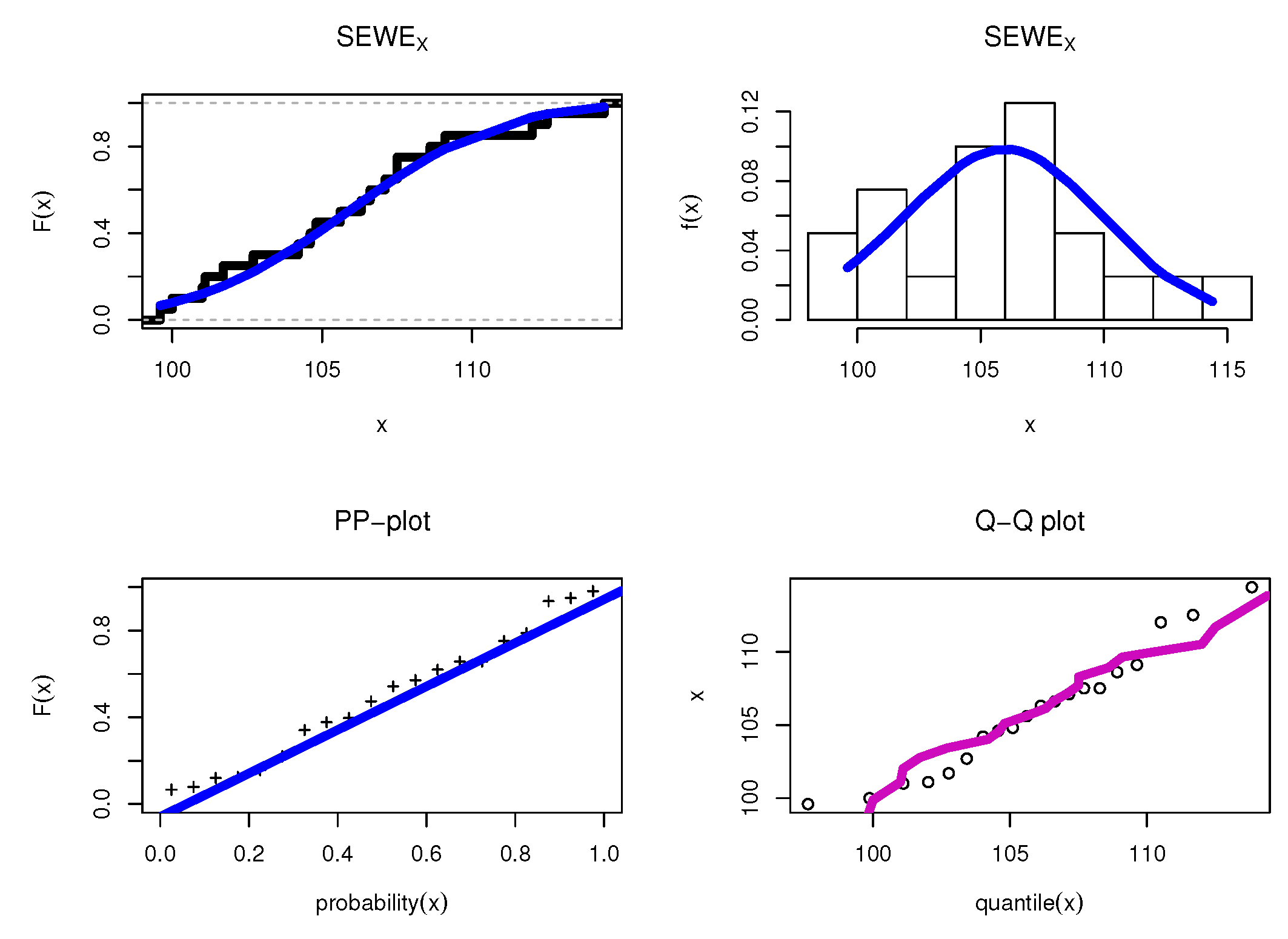
8.2. Wholesale Data
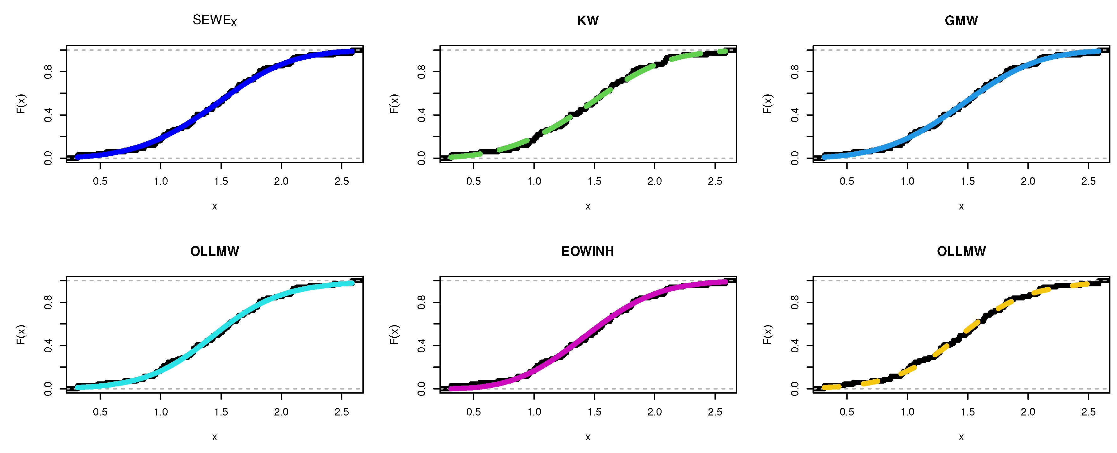
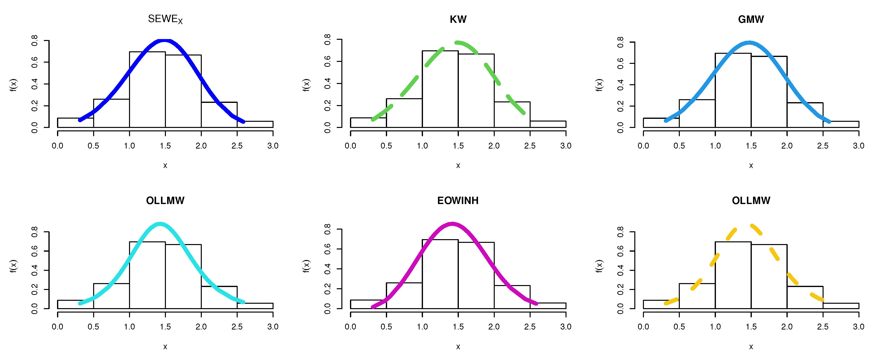
8.3. Single Carbon Fiber Data
8.4. Breaking Stress Dataset
8.5. TFP Growth Dataset
9. Conclusions and Summary
Author Contributions
Funding
Data Availability Statement
Acknowledgments
Conflicts of Interest
Appendix A

| E | E | E | E | E | E | |||||||||
|---|---|---|---|---|---|---|---|---|---|---|---|---|---|---|
| n | RBV | MSEV | RBV | MSEV | RBV | MSEV | RBV | MSEV | RBV | MSEV | RBV | MSEV | ||
| 0.5 | 40 | −0.0051 | 0.0065 | 0.0005 | 0.0008 | −0.0014 | 0.0013 | −0.0051 | 0.0048 | 0.0023 | 0.0008 | 0.0005 | 0.0009 | |
| −0.0786 | 0.0226 | 0.0029 | 0.0118 | −0.0030 | 0.0135 | −0.0786 | 0.0263 | 0.0350 | 0.0130 | 0.0059 | 0.0120 | |||
| 0.0405 | 0.0963 | −0.0073 | 0.0114 | −0.0102 | 0.0228 | 0.0407 | 0.1002 | −0.0185 | 0.0116 | −0.0167 | 0.0193 | |||
| 0.2161 | 0.0725 | 0.0180 | 0.0042 | 0.0540 | 0.0155 | 0.2154 | 0.0931 | 0.0136 | 0.0035 | 0.0446 | 0.0104 | |||
| 80 | −0.0032 | 0.0038 | −0.0005 | 0.0003 | 0.0009 | 0.0005 | −0.0032 | 0.0027 | 0.0003 | 0.0004 | −0.0003 | 0.0005 | ||
| −0.0553 | 0.0139 | −0.0021 | 0.0054 | −0.0028 | 0.0059 | −0.0552 | 0.0156 | 0.0046 | 0.0054 | −0.0057 | 0.0058 | |||
| 0.0412 | 0.0768 | 0.0028 | 0.0065 | 0.0140 | 0.0137 | 0.0413 | 0.0672 | −0.0008 | 0.0070 | 0.0039 | 0.0133 | |||
| 0.1263 | 0.0441 | 0.0135 | 0.0024 | 0.0141 | 0.0055 | 0.1259 | 0.0496 | 0.0108 | 0.0023 | 0.0253 | 0.0068 | |||
| 160 | −0.0008 | 0.0016 | −0.0001 | 0.0003 | 0.0002 | 0.0003 | −0.0008 | 0.0016 | 0.0002 | 0.0003 | −0.0001 | 0.0005 | ||
| −0.0298 | 0.0087 | −0.0021 | 0.0048 | −0.0001 | 0.0035 | −0.0300 | 0.0091 | 0.0048 | 0.0050 | −0.0035 | 0.0054 | |||
| 0.0567 | 0.0494 | 0.0027 | 0.0049 | 0.0108 | 0.0073 | 0.0406 | 0.0490 | 0.0006 | 0.0069 | 0.0035 | 0.0127 | |||
| 0.0483 | 0.0223 | 0.0129 | 0.0024 | 0.0046 | 0.0025 | 0.0486 | 0.0230 | 0.0131 | 0.0022 | 0.0203 | 0.0067 | |||
| 3 | 40 | −0.0053 | 0.3367 | −0.0011 | 0.0141 | 0.0090 | 0.0331 | −0.0051 | 0.2493 | 0.0010 | 0.0168 | 0.0039 | 0.0312 | |
| −0.0041 | 0.0103 | 0.0082 | 0.0098 | 0.0144 | 0.0084 | −0.0043 | 0.0069 | 0.0392 | 0.0114 | 0.0201 | 0.0080 | |||
| 0.1231 | 0.2721 | −0.0038 | 0.0126 | 0.0280 | 0.0278 | 0.1231 | 0.1563 | −0.0162 | 0.0125 | 0.0086 | 0.0187 | |||
| −0.0199 | 0.4947 | 0.0017 | 0.0267 | −0.0128 | 0.0609 | −0.0200 | 0.4374 | 0.0012 | 0.0278 | −0.0055 | 0.0541 | |||
| 80 | −0.0009 | 0.1493 | 0.0011 | 0.0132 | −0.0026 | 0.0268 | −0.0049 | 0.1569 | 0.0010 | 0.0138 | 0.0036 | 0.0161 | ||
| −0.0089 | 0.0038 | −0.0061 | 0.0043 | 0.0009 | 0.0036 | −0.0042 | 0.0032 | 0.0083 | 0.0044 | 0.0025 | 0.0034 | |||
| 0.0936 | 0.0744 | 0.0032 | 0.0093 | 0.0079 | 0.0136 | 0.0936 | 0.0890 | 0.0069 | 0.0081 | 0.0072 | 0.0126 | |||
| −0.0195 | 0.2347 | −0.0013 | 0.0243 | 0.0019 | 0.0483 | −0.0196 | 0.2829 | −0.0015 | 0.0237 | −0.0049 | 0.0316 | |||
| 160 | 0.0120 | 0.1345 | −0.0001 | 0.0026 | 0.0021 | 0.0128 | 0.0012 | 0.0895 | 0.0004 | 0.0038 | 0.0014 | 0.0106 | ||
| −0.0100 | 0.0025 | −0.0021 | 0.0031 | 0.0006 | 0.0024 | −0.0010 | 0.0021 | 0.0080 | 0.0032 | 0.0022 | 0.0024 | |||
| 0.0923 | 0.0733 | 0.0031 | 0.0032 | 0.0071 | 0.0061 | 0.0919 | 0.0516 | 0.0017 | 0.0034 | 0.0106 | 0.0068 | |||
| −0.0297 | 0.2404 | 0.0001 | 0.0044 | −0.0014 | 0.0221 | −0.0130 | 0.1752 | 0.0000 | 0.0063 | −0.0025 | 0.0193 | |||
| E | E | E | E | E | E | |||||||||
|---|---|---|---|---|---|---|---|---|---|---|---|---|---|---|
| n | RBV | MSEV | RBV | MSEV | RBV | MSEV | RBV | MSEV | RBV | MSEV | RBV | MSEV | ||
| 0.5 | 40 | −0.0436 | 0.4199 | −0.0074 | 0.0834 | −0.0027 | 0.0220 | −0.0435 | 0.3166 | −0.0032 | 0.0935 | −0.0041 | 0.1598 | |
| 0.0194 | 0.0322 | 0.0152 | 0.0093 | 0.0148 | 0.0075 | 0.0191 | 0.0176 | 0.0421 | 0.0113 | 0.0283 | 0.0100 | |||
| −0.0099 | 0.2653 | −0.0052 | 0.0554 | −0.0017 | 0.0123 | −0.0198 | 0.1630 | −0.0033 | 0.0580 | 0.0031 | 0.0936 | |||
| −0.0382 | 0.0089 | −0.0062 | 0.0042 | 0.0013 | 0.0033 | −0.0387 | 0.0048 | 0.0258 | 0.0045 | 0.0019 | 0.0035 | |||
| 80 | −0.0234 | 0.2154 | −0.0013 | 0.0643 | −0.0017 | 0.0076 | −0.0233 | 0.1976 | −0.0016 | 0.0841 | 0.0040 | 0.0916 | ||
| 0.0023 | 0.0124 | −0.0059 | 0.0036 | 0.0084 | 0.0033 | 0.0182 | 0.0091 | 0.0077 | 0.0038 | 0.0031 | 0.0032 | |||
| 0.0014 | 0.1411 | −0.0013 | 0.0105 | −0.0008 | 0.0037 | 0.0164 | 0.1059 | −0.0016 | 0.0163 | 0.0020 | 0.0198 | |||
| −0.0313 | 0.0054 | −0.0027 | 0.0019 | −0.0005 | 0.0016 | −0.0314 | 0.0030 | 0.0075 | 0.0020 | −0.0009 | 0.0016 | |||
| 160 | −0.0026 | 0.1627 | −0.0008 | 0.0144 | −0.0015 | 0.0068 | −0.0027 | 0.1034 | −0.0015 | 0.0167 | 0.0006 | 0.0339 | ||
| −0.0118 | 0.0049 | −0.0013 | 0.0028 | 0.0015 | 0.0022 | −0.0117 | 0.0032 | 0.0068 | 0.0029 | 0.0022 | 0.0025 | |||
| 0.0145 | 0.0984 | −0.0011 | 0.0099 | −0.0006 | 0.0036 | 0.0145 | 0.0691 | −0.0016 | 0.0108 | 0.0017 | 0.0123 | |||
| −0.0332 | 0.0025 | −0.0004 | 0.0014 | 0.0002 | 0.0011 | −0.0334 | 0.0021 | 0.0065 | 0.0015 | 0.0007 | 0.0013 | |||
| 3 | 40 | −0.0687 | 1.5287 | −0.0094 | 0.0275 | 0.0055 | 0.2252 | −0.0684 | 0.8406 | −0.0585 | 0.0237 | −0.0073 | 0.0911 | |
| 0.1085 | 0.2062 | 0.0097 | 0.0100 | 0.0241 | 0.0148 | 0.1080 | 0.0950 | 0.0424 | 0.0120 | 0.0259 | 0.0097 | |||
| −0.0277 | 0.4156 | −0.0091 | 0.0491 | 0.0047 | 0.0940 | −0.0278 | 0.2324 | 0.0096 | 0.0491 | 0.0012 | 0.0586 | |||
| −0.0358 | 0.1394 | −0.0036 | 0.0345 | −0.0037 | 0.0410 | −0.0360 | 0.0744 | 0.0143 | 0.0393 | 0.0033 | 0.0300 | |||
| 80 | −0.0467 | 0.9585 | −0.0019 | 0.0275 | −0.0073 | 0.1440 | −0.0465 | 0.4781 | −0.0078 | 0.0153 | −0.0041 | 0.0916 | ||
| 0.0440 | 0.0741 | −0.0043 | 0.0050 | 0.0162 | 0.0149 | 0.0438 | 0.0361 | 0.0142 | 0.0057 | 0.0066 | 0.0062 | |||
| −0.0158 | 0.2451 | −0.0046 | 0.0249 | −0.0048 | 0.0621 | −0.0159 | 0.1192 | −0.0063 | 0.0341 | 0.0012 | 0.0396 | |||
| −0.0253 | 0.0718 | −0.0032 | 0.0178 | 0.0009 | 0.0227 | −0.0253 | 0.0423 | 0.0051 | 0.0189 | −0.0013 | 0.0205 | |||
| 160 | −0.0153 | 0.4215 | −0.0015 | 0.0175 | −0.0063 | 0.0682 | −0.0155 | 0.2706 | −0.0045 | 0.0108 | −0.0035 | 0.0893 | ||
| 0.0060 | 0.0168 | 0.0037 | 0.0039 | 0.0085 | 0.0051 | 0.0061 | 0.0097 | 0.0132 | 0.0042 | 0.0062 | 0.0060 | |||
| −0.0016 | 0.1069 | −0.0033 | 0.0140 | −0.0009 | 0.0243 | −0.0017 | 0.0825 | 0.0018 | 0.0318 | −0.0010 | 0.0259 | |||
| −0.0237 | 0.0315 | 0.0012 | 0.0136 | 0.0004 | 0.0124 | −0.0239 | 0.0336 | 0.0045 | 0.0150 | 0.0012 | 0.0194 | |||
| E | E | E | E | E | E | |||||||||
|---|---|---|---|---|---|---|---|---|---|---|---|---|---|---|
| 0.5 | 40 | −0.01121 | 0.03921 | −0.00557 | 0.00859 | −0.00381 | 0.01597 | −0.01126 | 0.01443 | 0.00544 | 0.01353 | 0.00411 | 0.01517 | |
| −0.02074 | 0.05917 | 0.00910 | 0.02844 | −0.00946 | 0.02595 | −0.02086 | 0.04968 | 0.01512 | 0.03550 | 0.00706 | 0.04065 | |||
| 0.00108 | 0.00050 | −0.00027 | 0.00012 | −0.00019 | 0.00025 | 0.00109 | 0.00021 | −0.00125 | 0.00022 | −0.00041 | 0.00021 | |||
| −0.01047 | 0.00018 | −0.00231 | 0.00016 | −0.00391 | 0.00014 | −0.01057 | 0.00020 | 0.00220 | 0.00015 | −0.00031 | 0.00015 | |||
| 80 | −0.00782 | 0.03262 | −0.00246 | 0.00646 | 0.00328 | 0.00878 | −0.00784 | 0.00683 | 0.00330 | 0.00886 | −0.00136 | 0.01373 | ||
| −0.01516 | 0.02808 | −0.00515 | 0.01619 | 0.00809 | 0.01861 | −0.01519 | 0.02192 | 0.00417 | 0.01970 | −0.00504 | 0.02411 | |||
| 0.00085 | 0.00050 | 0.00017 | 0.00007 | −0.00077 | 0.00011 | 0.00085 | 0.00009 | −0.00038 | 0.00011 | 0.00037 | 0.00016 | |||
| −0.00590 | 0.00009 | −0.00177 | 0.00009 | 0.00223 | 0.00008 | −0.00592 | 0.00009 | 0.00150 | 0.00010 | −0.00028 | 0.00009 | |||
| 160 | −0.00507 | 0.00652 | −0.00085 | 0.00175 | −0.00123 | 0.00323 | −0.00509 | 0.00388 | 0.00081 | 0.00173 | −0.00064 | 0.00189 | ||
| −0.01107 | 0.01619 | −0.00123 | 0.00619 | −0.00147 | 0.00856 | −0.01109 | 0.01347 | 0.00156 | 0.00652 | −0.00167 | 0.00679 | |||
| 0.00067 | 0.00009 | 0.00001 | 0.00002 | −0.00010 | 0.00005 | 0.00067 | 0.00005 | −0.00013 | 0.00002 | 0.00011 | 0.00002 | |||
| −0.00413 | 0.00006 | −0.00018 | 0.00005 | −0.00021 | 0.00005 | −0.00417 | 0.00006 | 0.00106 | 0.00005 | −0.00013 | 0.00005 | |||
| 3 | 40 | −0.02534 | 0.77945 | −0.00540 | 0.04216 | −0.02703 | 0.20585 | −0.02518 | 0.69258 | 0.01059 | 0.04814 | 0.00493 | 0.06843 | |
| 0.02476 | 0.32320 | 0.00587 | 0.09164 | 0.02061 | 0.13155 | 0.02441 | 0.33022 | 0.02969 | 0.10620 | 0.01548 | 0.08509 | |||
| −0.00364 | 0.01487 | −0.00160 | 0.00058 | −0.00235 | 0.00319 | −0.00362 | 0.01415 | −0.00134 | 0.00062 | −0.00121 | 0.00103 | |||
| −0.01226 | 0.00699 | −0.00307 | 0.00931 | −0.00151 | 0.00793 | −0.01235 | 0.00856 | 0.00415 | 0.00925 | 0.00144 | 0.00731 | |||
| 80 | −0.01514 | 0.61948 | −0.00496 | 0.02314 | 0.01265 | 0.09885 | −0.01502 | 0.46116 | −0.00125 | 0.03397 | −0.00456 | 0.05829 | ||
| 0.00867 | 0.31488 | −0.00473 | 0.05100 | −0.00403 | 0.05293 | 0.00850 | 0.20105 | 0.00856 | 0.05780 | 0.00614 | 0.06378 | |||
| −0.00136 | 0.01230 | −0.00070 | 0.00042 | 0.00123 | 0.00165 | −0.00135 | 0.00891 | −0.00082 | 0.00061 | −0.00098 | 0.00100 | |||
| −0.00795 | 0.00375 | −0.00301 | 0.00445 | −0.00074 | 0.00383 | −0.00797 | 0.00396 | 0.00160 | 0.00439 | −0.00129 | 0.00362 | |||
| 160 | 0.00461 | 0.21543 | 0.00208 | 0.02135 | 0.00069 | 0.02479 | 0.00433 | 0.29192 | 0.00105 | 0.03412 | 0.00396 | 0.04742 | ||
| −0.00775 | 0.09234 | −0.00280 | 0.03551 | 0.00059 | 0.02697 | −0.00766 | 0.11092 | 0.00549 | 0.03685 | −0.00070 | 0.04183 | |||
| 0.00126 | 0.00390 | 0.00010 | 0.00036 | −0.00011 | 0.00036 | 0.00121 | 0.00540 | 0.00008 | 0.00057 | 0.00091 | 0.00096 | |||
| −0.00553 | 0.00234 | −0.00098 | 0.00325 | −0.00012 | 0.00262 | −0.00558 | 0.00278 | 0.00139 | 0.00326 | 0.00021 | 0.00257 | |||
References
- Marshall, A.; Olkin, I. A new method for adding a parameter to a class of distributions with applications to the exponential and Weibull families. Biometrika 1997, 84, 641–652. [Google Scholar] [CrossRef]
- Haq, A.; Elgarhy, M. The odd Fréchet-G class of probability distributions. J. Stat. Appl. Probab. 2018, 7, 189–203. [Google Scholar] [CrossRef]
- Eugene, N.; Lee, C.; Famoye, F. Beta-normal distribution and its applications. Commun. Stat. Theory Methods 2002, 31, 497–512. [Google Scholar] [CrossRef]
- Liu, M.; Ilyas, S.K.; Khosa, S.K.; Muhmoudi, E.; Ahmad, Z.; Khan, D.M.; Hamedani, G.G. A flexible reduced logarithmic-X family of distributions with biomedical analysis. Comput. Math. Methods Med. 2020, 2020, 4373595. [Google Scholar] [CrossRef] [Green Version]
- Muhammad, M.; Bantan, R.A.R.; Liu, L.; Chesneau, C.; Tahir, M.H.; Jamal, F.; Elgarhy, M. A New Extended Cosine—G Distributions for Life time Studies. Mathematics 2021, 9, 2758. [Google Scholar] [CrossRef]
- He, W.; Ahmad, Z.; Afify, A.Z.; Goual, H. The arcsine exponentiated-X family: Validation and insurance application. Complexity 2020, 2020, 8394815. [Google Scholar] [CrossRef]
- Alotaibi, N.; Elbatal, I.; Almetwally, E.M.; Alyami, S.A.; Al-Moisheer, A.S.; Elgarhy, M. Truncated Cauchy Power Weibull-G Class of Distributions: Bayesian and Non-Bayesian Inference Modelling for COVID-19 and Carbon Fiber Data. Mathematics 2022, 10, 1565. [Google Scholar] [CrossRef]
- Afify, A.Z.; Altun, E.; Alizadeh, M.; Ozel, G.; Hamedani, G.G. The odd exponentiated half-logistic-G class: Properties, characterizations and applications. Chil. J. Stat. 2017, 8, 65–91. [Google Scholar]
- Nofal, Z.M.; Afify, A.Z.; Yousof, H.M.; Cordeiro, G.M. The generalized transmuted-G family of distributions. Commun. Stat. Theory Methods 2017, 46, 4119–4136. [Google Scholar] [CrossRef]
- Cordeiro, G.M.; Alizadeh, M.; Ozel, G.; Hosseini, B.; Ortega, E.M.M.; Altun, E. The generalized odd log-logistic class of distributions: Properties, regression models and applications. J. Stat. Comput. Simul. 2017, 87, 908–932. [Google Scholar] [CrossRef]
- Badr, M.; Elbatal, I.; Jamal, F.; Chesneau, C.; Elgarhy, M. The Transmuted Odd Fréchet-G class of Distributions: Theory and Applications. Mathematics 2020, 8, 958. [Google Scholar] [CrossRef]
- Tahir, M.H.; Cordeiro, G.M.; Alzaatreh, A.; Mansoor, M.; Zubair, M. The Logistic-X class of distributions and its Applications. Commun. Stat. Theory Method 2016, 45, 7326–7349. [Google Scholar] [CrossRef] [Green Version]
- Jamal, F.; Chesneau, C.; Bouali, D.L.; Ul Hassan, M. Beyond the Sin-G family: The transformed Sin-G family. PLoS ONE 2021, 16, e0250790. [Google Scholar] [CrossRef]
- Souza, L.; Junior, W.R.O.; de Brito, C.C.R.; Chesneau, C.; Ferreira, T.A.E.; Soares, L. General properties for the Cos-G class ofdistributions with applications. Eurasian Bull. Math. 2019, 2, 63–79. [Google Scholar]
- Elbatal, I.; Alotaibi, N.; Almetwally, E.M.; Alyami, S.A.; Elgarhy, M. On Odd Perks-G Class of Distributions: Properties, Regression Model, Discretization, Bayesian and Non-Bayesian Estimation, and Applications. Symmetry 2022, 14, 883. [Google Scholar] [CrossRef]
- Jamal, F.; Chesneau, C.; Saboor, A.; Aslam, M.; Tahit, M.H.; Mashwan, W.K. The U Family of Distributions: Properties and applicantions. Math. Slov. 2022, 72, 17–240. [Google Scholar] [CrossRef]
- Nasiru, S. Extended Odd Fréchet-G class of Distributions. J. Probab. Stat. 2018, 2018, 2931326. [Google Scholar] [CrossRef]
- Bantan, R.A.; Chesneau, C.; Jamal, F.; Elgarhy, M. On the analysis of new COVID-19 cases in Pakistan using an exponentiated version of the M family of distributions. Mathematics 2020, 8, 953. [Google Scholar] [CrossRef]
- Afify, A.Z.; Alizadeh, M.; Yousof, H.M.; Aryal, G.; Ahmad, M. The transmuted geometric-G family of distributions: Theory and applications. Pak. J. Stat. 2016, 32, 139–160. [Google Scholar]
- Algarni, A.; Almarashi, A.M.; Elbatal, I.; Hassan, A.S.; Almetwally, E.M.; Daghistani, A.M.; Elgarhy, M. Type I half logis-tic Burr X-G family: Properties, Bayesian, and non-Bayesian estimation under censored samples and applications to COVID-19 data. Math. Probl. Eng. 2021, 2021, 5461130. [Google Scholar] [CrossRef]
- Mahmood, Z.; Chesneau, C.; Tahir, M.H. A new sine-G family of distributions: Properties and applications. Bull. Comput. Appl. Math. 2019, 7, 53–81. [Google Scholar]
- Almarashi, A.M.; Jamal, F.; Chesneau, C.; Elgarhy, M. The Exponentiated truncated inverse Weibull-generated family of distributions with applications. Symmetry 2020, 12, 650. [Google Scholar] [CrossRef] [Green Version]
- Yousof, H.M.; Afify, A.Z.; Hamedani, G.G.; Aryal, G. The Burr X generator of distributions for lifetime data. J. Stat. Theory Appl. 2017, 16, 288–305. [Google Scholar] [CrossRef] [Green Version]
- Souza, L.; de Oliveira, W.R.; de Brito, C.C.R.; Chesneau, C.; Fernandes, R.; Ferreira, T.A.E. Sec-GClass of Distributions: Properties andApplications. Symmetry 2022, 14, 299. [Google Scholar] [CrossRef]
- Nascimento, A.; Silva, K.F.; Cordeiro, M.; Alizadeh, M.; Yousof, H.; Hamedani, G. The odd Nadarajah–Haghighi family of distributions. Prop. Appl. Stud. Sci. Math. Hung. 2019, 56, 1–26. [Google Scholar]
- Al-Shomrani, A.; Arif, O.; Shawky, A.; Hanif, S.; Shahbaz, M.Q. Topp–Leone family of distributions: Some properties and application. Pak. J. Stat. Oper. Res. 2016, 12, 443–451. [Google Scholar] [CrossRef] [Green Version]
- Al-Babtain, A.A.; Elbatal, I.; Chesneau, C.; Elgarhy, M. Sine Topp-Leone-G family of distributions: Theory and applications. Open Phys. 2020, 18, 74–593. [Google Scholar] [CrossRef]
- Bantan, R.A.; Jamal, F.; Chesneau, C.; Elgarhy, M. A New Power Topp–Leone Generated Family of Distributions with Applications. Entropy 2019, 21, 1177. [Google Scholar] [CrossRef] [Green Version]
- Bantan, R.A.; Jamal, F.; Chesneau, C.; Elgarhy, M. Truncated inverted Kumaraswamy generated family of distributions with applications. Entropy 2019, 21, 1089. [Google Scholar] [CrossRef] [Green Version]
- Cordeiro, G.M.; Afify, A.Z.; Yousof, H.M.; Pescim, R.R.; Aryal, G.R. The Exponentiated Weibull-H Family of Distributions: Theory and Applications. Mediterr. J. Math. 2013, 71, 955. [Google Scholar] [CrossRef]
- Bourguignon, M.; Silva, R.B.; Cordeiro, G.M. The Weibull-G family of probability distributions. J. Data Sci. 2014, 12, 1253–1268. [Google Scholar] [CrossRef]
- Kumar, D.; Singh, U.; Singh, S.K. A New Distribution Using Sine Function Its Application to Bladder Cancer Patients Data. J. Stat. Appl. Probl. 2015, 4, 417–427. [Google Scholar]
- Nadarajah, S.; Kotz, S. Beta Trigonometric Distribution. Port. Econ. J. 2006, 3, 207–224. [Google Scholar] [CrossRef]
- Al-Faris, R.Q.; Khan, S. Sine Square distribution: A New Statistical Model Based on the Sine Function. J. Appl. Probab. Stat. 2008, 3, 163–173. [Google Scholar]
- Raab, D.H.; Green, E.H. A cosine approximation to the normal distribution. Psychometrika 1961, 26, 447–450. [Google Scholar] [CrossRef]
- Kharazmi, O.; Saadatinik, A.; Jahangard, S. Odd Hyperbolic Cosine Exponential-Exponential (OHC-EE) Distribution. Ann. Data Sci. 2019, 6, 1–21. [Google Scholar] [CrossRef] [Green Version]
- Souza, L. New Trigonometric Classes of Probabilistic Distributions. Ph.D. Thesis, Universidade Federal Rural de Pernambuco, Recife, Brazil, 2015. [Google Scholar]
- Kharazmi, O.; Saadatinik, A.; Alizadeh, M.; Hamedani, G.G. Odd hyperbolic cosine family of lifetime distributions. J. Stat. Theory Appl. 2018, 4, 387–401. [Google Scholar] [CrossRef] [Green Version]
- Bleed, S.O.; Abdelali, A.E. Transmuted Arcsine Distribution Properties and Application. Int. J. Res. 2018, 6, 1–11. [Google Scholar] [CrossRef]
- Ibrahim, G.M.; Hassan, A.S.; Almetwally, E.M.; Almongy, H.M. Parameter estimation of alpha power inverted Topp-Leone distribution with applications. Intell. Autom. Soft Comput. 2021, 29, 353–371. [Google Scholar] [CrossRef]
- Almetwally, E.M. The odd Weibull inverse topp–leone distribution with applications to COVID-19 data. Ann. Data Sci. 2022, 9, 121–140. [Google Scholar] [CrossRef]
- Almetwally, E.M.; Ahmad, H.H. A new generalization of the Pareto distribution and its applications. Stat. Transit. N. Ser. 2020, 21, 61–84. [Google Scholar] [CrossRef]
- Basheer, A.M.; Almetwally, E.M.; Okasha, H.M. Marshall-olkin alpha power inverse Weibull distribution: Non bayesian and bayesian estimations. J. Stat. Appl. Probab. 2021, 10, 327–345. [Google Scholar]
- Ali, M.M.; Pal, M.; Woo, J. Estimation of P (Y< X) in a four-parameter generalized gamma distribution. Aust. J. Stat. 2012, 41, 197–210. [Google Scholar]
- Cordeiro, G.M.; Lemonte, A.J. The β-Birnbaum–Saunders distribution: An improved distribution for fatigue life modeling. Comput. Stat. Data Anal. 2011, 55, 1445–1461. [Google Scholar] [CrossRef]


| Model | |||
|---|---|---|---|
| SW-H family | - | - | 1 |
| SBX-H family | 1 | 2 | - |
| SEE-H family | - | 1 | - |
| SE-H family | - | 1 | 1 |
| 1.2 | 0.287 | 0.234 | 0.273 | 0.402 | 0.151 | 2.02 | 8.056 | 1.352 | |
| 1.5 | 0.333 | 0.299 | 0.370 | 0.567 | 0.189 | 1.773 | 6.64 | 1.305 | |
| 1.8 | 0.368 | 0.360 | 0.468 | 0.742 | 0.225 | 1.607 | 5.75 | 1.289 | |
| 0.7 | 2 | 0.386 | 0.397 | 0.533 | 0.862 | 0.248 | 1.527 | 5.327 | 1.289 |
| 2.3 | 0.409 | 0.448 | 0.627 | 1.044 | 0.281 | 1.437 | 4.853 | 1.297 | |
| 2.6 | 0.426 | 0.495 | 0.718 | 1.227 | 0.313 | 1.375 | 4.513 | 1.312 | |
| 3 | 0.444 | 0.550 | 0.834 | 1.469 | 0.353 | 1.322 | 4.194 | 1.339 | |
| 1.2 | 0.285 | 0.223 | 0.233 | 0.296 | 0.142 | 1.656 | 5.9 | 1.322 | |
| 1.5 | 0.315 | 0.273 | 0.305 | 0.404 | 0.174 | 1.496 | 5.051 | 1.326 | |
| 1.8 | 0.335 | 0.316 | 0.372 | 0.513 | 0.204 | 1.405 | 4.541 | 1.348 | |
| 0.9 | 2 | 0.345 | 0.34 | 0.415 | 0.585 | 0.223 | 1.368 | 4.311 | 1.369 |
| 2.3 | 0.355 | 0.375 | 0.475 | 0.691 | 0.249 | 1.336 | 4.072 | 1.403 | |
| 2.6 | 0.362 | 0.404 | 0.532 | 0.795 | 0.272 | 1.324 | 3.918 | 1.44 | |
| 3 | 0.368 | 0.436 | 0.600 | 0.928 | 0.301 | 1.326 | 3.798 | 1.49 | |
| 1.2 | 0.255 | 0.200 | 0.196 | 0.222 | 0.135 | 1.512 | 4.795 | 1.443 | |
| 1.5 | 0.266 | 0.232 | 0.242 | 0.288 | 0.161 | 1.467 | 4.414 | 1.505 | |
| 1.8 | 0.271 | 0.256 | 0.283 | 0.351 | 0.182 | 1.468 | 4.245 | 1.573 | |
| 1.2 | 2 | 0.273 | 0.27 | 0.307 | 0.391 | 0.195 | 1.482 | 4.2 | 1.619 |
| 2.3 | 0.273 | 0.286 | 0.340 | 0.447 | 0.211 | 1.514 | 4.194 | 1.685 | |
| 2.6 | 0.271 | 0.299 | 0.369 | 0.500 | 0.225 | 1.554 | 4.237 | 1.749 | |
| 3 | 0.268 | 0.312 | 0.403 | 0.564 | 0.240 | 1.612 | 4.34 | 1.828 | |
| 1.2 | 0.211 | 0.170 | 0.163 | 0.176 | 0.126 | 1.654 | 4.929 | 1.677 | |
| 1.5 | 0.211 | 0.188 | 0.192 | 0.218 | 0.143 | 1.701 | 4.901 | 1.792 | |
| 1.8 | 0.208 | 0.200 | 0.216 | 0.257 | 0.157 | 1.77 | 5.017 | 1.902 | |
| 1.5 | 2 | 0.205 | 0.21 | 0.230 | 0.280 | 0.164 | 1.821 | 5.136 | 1.971 |
| 2.3 | 0.201 | 0.213 | 0.248 | 0.311 | 0.172 | 1.899 | 5.352 | 2.069 | |
| 2.6 | 0.196 | 0.217 | 0.263 | 0.340 | 0.179 | 1.976 | 5.592 | 2.159 | |
| 3 | 0.19 | 0.222 | 0.279 | 0.373 | 0.186 | 2.074 | 5.93 | 2.268 | |
| 1.2 | 0.153 | 0.128 | 0.122 | 0.128 | 0.105 | 2.09 | 6.415 | 2.117 | |
| 1.5 | 0.145 | 0.134 | 0.137 | 0.152 | 0.113 | 2.239 | 6.919 | 2.308 | |
| 1.8 | 0.138 | 0.137 | 0.148 | 0.171 | 0.118 | 2.386 | 7.504 | 2.481 | |
| 1.9 | 2 | 0.134 | 0.14 | 0.154 | 0.182 | 0.120 | 2.479 | 7.91 | 2.586 |
| 2.3 | 0.128 | 0.139 | 0.161 | 0.197 | 0.122 | 2.611 | 8.524 | 2.731 | |
| 2.6 | 0.123 | 0.139 | 0.166 | 0.209 | 0.124 | 2.734 | 9.13 | 2.862 | |
| 3 | 0.117 | 0.138 | 0.172 | 0.223 | 0.124 | 2.882 | 9.916 | 3.018 | |
| 1.2 | 0.127 | 0.108 | 0.104 | 0.109 | 0.092 | 2.384 | 7.729 | 2.39 | |
| 1.5 | 0.119 | 0.111 | 0.114 | 0.126 | 0.097 | 2.583 | 8.588 | 2.626 | |
| 1.8 | 0.111 | 0.112 | 0.121 | 0.139 | 0.099 | 2.769 | 9.498 | 2.836 | |
| 2.1 | 2 | 0.107 | 0.11 | 0.125 | 0.147 | 0.100 | 2.885 | 10.107 | 2.962 |
| 2.3 | 0.101 | 0.111 | 0.129 | 0.157 | 0.101 | 3.046 | 11.006 | 3.135 | |
| 2.6 | 0.096 | 0.110 | 0.132 | 0.165 | 0.100 | 3.193 | 11.878 | 3.291 | |
| 3 | 0.091 | 0.108 | 0.134 | 0.174 | 0.100 | 3.37 | 12.991 | 3.476 |
| 1.2 | 1.015 | 1.965 | 5.278 | 17.352 | 0.935 | 1.532 | 5.589 | 0.953 | |
| 1.5 | 1.25 | 2.648 | 7.461 | 25.237 | 1.085 | 1.273 | 4.616 | 0.833 | |
| 1.8 | 1.462 | 3.331 | 9.782 | 33.946 | 1.195 | 1.088 | 4.036 | 0.748 | |
| 0.4 | 2 | 1.591 | 3.782 | 11.382 | 40.119 | 1.251 | 0.99 | 3.77 | 0.703 |
| 2.3 | 1.769 | 4.446 | 13.833 | 49.817 | 1.315 | 0.87 | 3.48 | 0.648 | |
| 2.6 | 1.932 | 5.092 | 16.321 | 59.937 | 1.361 | 0.772 | 3.277 | 0.604 | |
| 3 | 2.127 | 5.923 | 19.659 | 73.922 | 1.4 | 0.667 | 3.091 | 0.556 | |
| 1.2 | 1.456 | 3.008 | 7.622 | 22.215 | 0.887 | 0.788 | 3.293 | 0.647 | |
| 1.5 | 1.703 | 3.827 | 10.225 | 30.886 | 0.926 | 0.621 | 3.016 | 0.565 | |
| 1.8 | 1.911 | 4.592 | 12.819 | 39.928 | 0.938 | 0.502 | 2.873 | 0.507 | |
| 0.6 | 2 | 2.033 | 5.072 | 14.525 | 46.072 | 0.937 | 0.44 | 2.816 | 0.476 |
| 2.3 | 2.196 | 5.751 | 17.033 | 55.365 | 0.928 | 0.365 | 2.764 | 0.439 | |
| 2.6 | 2.339 | 6.384 | 19.469 | 64.674 | 0.913 | 0.306 | 2.737 | 0.408 | |
| 3 | 2.505 | 7.163 | 22.598 | 77.008 | 0.888 | 0.245 | 2.723 | 0.376 | |
| 1.2 | 1.795 | 4.008 | 10.28 | 29.141 | 0.785 | 0.384 | 2.694 | 0.493 | |
| 1.5 | 2.034 | 4.898 | 13.235 | 38.962 | 0.762 | 0.259 | 2.648 | 0.429 | |
| 1.8 | 2.227 | 5.691 | 16.036 | 48.721 | 0.73 | 0.174 | 2.65 | 0.384 | |
| 0.8 | 2 | 2.338 | 6.172 | 17.815 | 55.126 | 0.708 | 0.131 | 2.663 | 0.36 |
| 2.3 | 2.482 | 6.833 | 20.351 | 64.526 | 0.674 | 0.082 | 2.688 | 0.331 | |
| 2.6 | 2.606 | 7.432 | 22.739 | 73.647 | 0.643 | 0.044 | 2.715 | 0.308 | |
| 3 | 2.747 | 8.15 | 25.711 | 85.347 | 0.605 | 0.008 | 2.75 | 0.283 | |
| 1.2 | 2.056 | 4.901 | 12.914 | 36.675 | 0.675 | 0.119 | 2.565 | 0.4 | |
| 1.5 | 2.279 | 5.817 | 16.103 | 47.486 | 0.622 | 0.023 | 2.624 | 0.346 | |
| 1.8 | 2.456 | 6.603 | 19.013 | 57.817 | 0.573 | −0.039 | 2.687 | 0.308 | |
| 1 | 2 | 2.554 | 7.069 | 20.812 | 64.414 | 0.544 | −0.069 | 2.725 | 0.289 |
| 2.3 | 2.682 | 7.698 | 23.321 | 73.871 | 0.506 | −0.101 | 2.776 | 0.265 | |
| 2.6 | 2.79 | 8.256 | 25.629 | 82.823 | 0.472 | −0.123 | 2.818 | 0.246 | |
| 3 | 2.912 | 8.912 | 28.437 | 94.03 | 0.434 | −0.142 | 2.864 | 0.226 | |
| 1.2 | 2.163 | 5.303 | 14.177 | 40.471 | 0.623 | 0.017 | 2.574 | 0.365 | |
| 1.5 | 2.379 | 6.221 | 17.445 | 51.683 | 0.563 | −0.068 | 2.662 | 0.315 | |
| 1.8 | 2.547 | 6.997 | 20.378 | 62.221 | 0.511 | −0.12 | 2.741 | 0.281 | |
| 1.1 | 2 | 2.64 | 7.453 | 22.172 | 68.871 | 0.481 | −0.144 | 2.785 | 0.263 |
| 2.3 | 2.761 | 8.063 | 24.652 | 78.313 | 0.443 | −0.169 | 2.839 | 0.241 | |
| 2.6 | 2.862 | 8.6 | 26.911 | 87.16 | 0.41 | −0.185 | 2.882 | 0.224 | |
| 3 | 2.975 | 9.227 | 29.636 | 98.125 | 0.374 | −0.197 | 2.926 | 0.206 | |
| 1.2 | 2.421 | 6.35 | 17.672 | 51.513 | 0.49 | −0.214 | 2.722 | 0.289 | |
| 1.5 | 2.612 | 7.245 | 21.057 | 63.569 | 0.422 | −0.271 | 2.853 | 0.249 | |
| 1.8 | 2.758 | 7.978 | 23.981 | 74.443 | 0.37 | −0.301 | 2.945 | 0.221 | |
| 1.4 | 2 | 2.838 | 8.399 | 25.723 | 81.114 | 0.343 | −0.311 | 2.99 | 0.206 |
| 2.3 | 2.94 | 8.952 | 28.08 | 90.364 | 0.309 | −0.318 | 3.038 | 0.189 | |
| 2.6 | 3.025 | 9.431 | 30.182 | 98.823 | 0.281 | −0.32 | 3.072 | 0.175 | |
| 3 | 3.119 | 9.981 | 32.664 | 109.062 | 0.252 | −0.316 | 3.1 | 0.161 |
| AIC | BIC | CVMV | ADV | KSD | PVKS | ||||||
|---|---|---|---|---|---|---|---|---|---|---|---|
| SEWE | 25.4578 | 5.8544 | 0.0969 | 0.0100 | 105.5160 | 109.4989 | 0.0316 | 0.2317 | 0.0973 | 0.9915 | |
| 2.5656 | 0.6520 | 0.0416 | 0.0002 | ||||||||
| EGWGP | 12.9987 | 0.0028 | 0.2820 | 0.1226 | 0.9072 | 119.7390 | 124.7177 | 0.0325 | 0.2321 | 0.1969 | 0.4202 |
| 6.9675 | 0.0003 | 1.1229 | 0.0319 | 0.1267 | |||||||
| KEBXII | 200.4707 | 104.7107 | 1151.0364 | 44.4507 | 0.0386 | 137.3374 | 142.3161 | 0.0329 | 0.2400 | 0.3543 | 0.0132 |
| 91.5733 | 47.5651 | 823.2539 | 7.5603 | 0.0005 | |||||||
| WL | 39.6383 | 94.6265 | 0.2092 | 4.3605 | 108.0184 | 112.0013 | 0.0679 | 0.4812 | 0.1416 | 0.8177 | |
| 500.3255 | 5.4938 | 0.1859 | 1.3285 | ||||||||
| MOAPW | 8.6847 | 13.4815 | 14.5558 | 94.1638 | 108.9627 | 112.9457 | 0.0486 | 0.3695 | 0.1314 | 0.8800 | |
| 12.1874 | 3.3482 | 14.2031 | 3.8432 | ||||||||
| KW | 1.0714 | 0.0250 | 9.9170 | 0.5157 | 255.0566 | 259.0395 | 0.1066 | 0.6499 | 0.5813 | 0.0000 | |
| 0.0069 | 0.0056 | 0.0022 | 0.0014 | ||||||||
| ESW | 19.3720 | 1.2484 | 0.0054 | 174.1453 | 177.1325 | 0.0331 | 0.2310 | 0.4250 | 0.0015 | ||
| 7.4081 | 0.0472 | 0.0011 |
| AIC | BIC | CVMV | ADV | KSD | PVKS | ||||||
|---|---|---|---|---|---|---|---|---|---|---|---|
| SEWE | 27.5666 | 2.6193 | 0.0172 | 0.0201 | 121.2337 | 125.2167 | 0.0292 | 0.2512 | 0.0937 | 0.9947 | |
| 2.5646 | 1.5169 | 0.0073 | 0.0166 | ||||||||
| EGWGP | 39.1871 | 0.0038 | 8.5649 | 0.6128 | 0.9686 | 162.5654 | 167.5440 | 0.1286 | 0.7957 | 0.4030 | 0.0030 |
| 16.1161 | 0.0004 | 0.0057 | 0.0018 | 0.0012 | |||||||
| KEBXII | 537.5850 | 649.1720 | 375.1731 | 4.2158 | 0.5565 | 135.8559 | 140.8345 | 0.0318 | 0.2694 | 0.2525 | 0.1561 |
| 5.6995 | 21.6522 | 194.6549 | 0.3778 | 0.0499 | |||||||
| WL | 0.0025 | 45.0467 | 0.3496 | 13.7505 | 124.2758 | 128.2587 | 0.0720 | 0.5231 | 0.1491 | 0.7653 | |
| 0.0007 | 3.7874 | 0.1985 | 1.3843 | ||||||||
| MOAPW | 378.1695 | 5.1839 | 449.6787 | 71.0195 | 123.1665 | 127.1494 | 0.0369 | 0.3183 | 0.1064 | 0.9774 | |
| 1288.6846 | 1.5231 | 948.4074 | 11.2737 | ||||||||
| KW | 1.0993 | 0.0279 | 10.0478 | 0.5114 | 256.5495 | 260.5324 | 0.0632 | 0.4927 | 0.6143 | 0.0000 | |
| 0.0032 | 0.0062 | 0.0034 | 0.0013 | ||||||||
| ESW | 20.8703 | 1.3592 | 0.0032 | 171.1671 | 174.1543 | 0.0268 | 0.2254 | 0.4003 | 0.0033 | ||
| 8.1773 | 0.0295 | 0.0003 |
| AIC | BIC | KSD | PVKS | CVMV | ADV | ||||||
|---|---|---|---|---|---|---|---|---|---|---|---|
| SEWE | estimates | 14.2450 | 0.2028 | 1.1062 | 2.9008 | 105.2991 | 114.2356 | 0.0403 | 0.9999 | 0.0172 | 0.1557 |
| SE | 7.1414 | 0.1436 | 1.0753 | 1.4375 | |||||||
| OLLMW | estimates | 28.7708 | 0.0560 | 0.6093 | 0.0125 | 106.6756 | 115.6121 | 0.0468 | 0.9982 | 0.0222 | 0.1625 |
| SE | 39.8918 | 0.0814 | 0.1193 | 0.0310 | |||||||
| KW | estimates | 0.7560 | 0.1473 | 1.0575 | 3.4344 | 105.5197 | 114.4561 | 0.0487 | 0.9967 | 0.0220 | 0.1947 |
| SE | 0.0286 | 0.0202 | 0.0209 | 0.0151 | |||||||
| GMW | estimates | 0.4879 | 4.4450 | 0.8570 | 0.3466 | 105.4390 | 114.3755 | 0.0422 | 0.9997 | 0.0185 | 0.1654 |
| SE | 0.7596 | 8.9394 | 0.2829 | 1.0786 | |||||||
| EOWL | estimates | 2.6361 | 0.1152 | 8.7047 | 19.2595 | 105.5875 | 114.5240 | 0.0435 | 0.9995 | 0.0211 | 0.1878 |
| SE | 0.4997 | 0.2885 | 43.9097 | 100.6442 | |||||||
| EOWINH | estimates | 3.2607 | 0.0821 | 0.5014 | 2.9358 | 109.0365 | 117.9729 | 0.0424 | 0.9997 | 0.0405 | 0.3270 |
| SE | 1.2895 | 0.3173 | 0.2179 | 1.9671 |
| AIC | BIC | KSD | PVKS | CVMV | ADV | ||||||
|---|---|---|---|---|---|---|---|---|---|---|---|
| SEWE | estimates | 24.8869 | 0.0945 | 1.4235 | 3.0217 | 178.4290 | 187.1876 | 0.0707 | 0.8967 | 0.0631 | 0.3704 |
| SE | 75.6618 | 0.1957 | 2.3635 | 4.4106 | |||||||
| OLLMW | estimates | 2.761189 | 0.140337 | 0.054904 | 1.73303 | 182.6582 | 191.4168 | 0.0835 | 0.7467 | 0.1416 | 0.7459 |
| SE | 25.9085 | 0.0357 | 0.0977 | 0.0260 | |||||||
| KW | estimates | 0.7246 | 0.1677 | 0.5057 | 3.8408 | 179.2803 | 188.0390 | 0.0841 | 0.7392 | 0.0730 | 0.4549 |
| SE | 0.0144 | 0.0244 | 0.0102 | 0.0170 | |||||||
| GMW | estimates | 0.4364 | 5.4989 | 0.5161 | 0.1485 | 178.7462 | 187.5048 | 0.0761 | 0.8398 | 0.0654 | 0.3940 |
| SE | 0.6527 | 8.0561 | 0.1731 | 0.5409 | |||||||
| EOWINH | estimates | 4.5935 | 0.0028 | 0.2527 | 21.5314 | 180.3045 | 189.0631 | 0.0832 | 0.7515 | 0.0946 | 0.5382 |
| SE | 1.9504 | 0.2126 | 0.1221 | 24.5623 |
| AIC | BIC | CVMV | ADV | KSD | PVKS | |||||||
|---|---|---|---|---|---|---|---|---|---|---|---|---|
| SEWE | estimates | 18.9511 | 0.2121 | 2.6809 | 0.6078 | 114.7737 | 116.0237 | 0.0329 | 0.1988 | 0.0826 | 0.9622 | |
| SE | 686.6481 | 3.1465 | 27.8125 | 5.5706 | ||||||||
| EGWGP | estimates | 0.9855 | 0.6312 | 1.3171 | 0.4959 | 0.0860 | 116.8016 | 118.7371 | 0.0332 | 0.1994 | 0.0830 | 0.9618 |
| SE | 4.0934 | 4.3180 | 0.4487 | 0.2928 | 0.9245 | |||||||
| KEBXII | estimates | 39.6448 | 1.1351 | 569.6257 | 0.1379 | 2.7644 | 117.6760 | 119.6115 | 0.0385 | 0.2376 | 0.1061 | 0.7991 |
| SE | 81.7057 | 2.3102 | 1917.6428 | 0.1862 | 4.2189 | |||||||
| WL | estimates | 2.6661 | 1.3872 | 1.1264 | 4.3821 | 114.9927 | 116.2427 | 0.0330 | 0.1989 | 0.0828 | 0.9622 | |
| SE | 73.0566 | 0.5367 | 4.0920 | 102.3363 | ||||||||
| MOAPW | estimates | 0.9331 | 1.4697 | 0.8656 | 2.0064 | 114.9835 | 116.2335 | 0.0340 | 0.1989 | 0.0843 | 0.9550 | |
| SE | 9.1323 | 0.4757 | 4.3685 | 1.1887 | ||||||||
| KW | estimates | 3.1522 | 0.1048 | 5.1531 | 1.0782 | 116.6211 | 117.8711 | 0.0566 | 0.3540 | 0.1279 | 0.5805 | |
| SE | 0.0914 | 0.0174 | 0.0097 | 0.0095 | ||||||||
| 1.0655 | 1.2939 | 0.2672 | 113.0408 | 113.7681 | 0.0289 | 0.1795 | 0.0793 | 0.9741 | ||||
| 0.7932 | 0.5831 | 0.2602 |
Publisher’s Note: MDPI stays neutral with regard to jurisdictional claims in published maps and institutional affiliations. |
© 2022 by the authors. Licensee MDPI, Basel, Switzerland. This article is an open access article distributed under the terms and conditions of the Creative Commons Attribution (CC BY) license (https://creativecommons.org/licenses/by/4.0/).
Share and Cite
Alyami, S.A.; Elbatal, I.; Alotaibi, N.; Almetwally, E.M.; Elgarhy, M. Modeling to Factor Productivity of the United Kingdom Food Chain: Using a New Lifetime-Generated Family of Distributions. Sustainability 2022, 14, 8942. https://doi.org/10.3390/su14148942
Alyami SA, Elbatal I, Alotaibi N, Almetwally EM, Elgarhy M. Modeling to Factor Productivity of the United Kingdom Food Chain: Using a New Lifetime-Generated Family of Distributions. Sustainability. 2022; 14(14):8942. https://doi.org/10.3390/su14148942
Chicago/Turabian StyleAlyami, Salem A., Ibrahim Elbatal, Naif Alotaibi, Ehab M. Almetwally, and Mohammed Elgarhy. 2022. "Modeling to Factor Productivity of the United Kingdom Food Chain: Using a New Lifetime-Generated Family of Distributions" Sustainability 14, no. 14: 8942. https://doi.org/10.3390/su14148942