
Optimal Power Flow Solution of Power Systems with Renewable Energy Sources Using White Sharks Algorithm


1
Department of Electrical Engineering, Faculty of Engineering, Azhar University, Qena 83513, Egypt
2
Department of Electrical Engineering, Faculty of Engineering, Aswan University, Aswan 81542, Egypt
3
Department of Electrical Engineering, College of Engineering, Jouf University, Sakaka 72388, Saudi Arabia
*
Author to whom correspondence should be addressed.
Sustainability 2022, 14(10), 6049; https://doi.org/10.3390/su14106049
Submission received: 26 March 2022
/
Revised: 10 May 2022
/
Accepted: 13 May 2022
/
Published: 16 May 2022
(This article belongs to the Section Resources and Sustainable Utilization)
Abstract
:Modern electrical power systems are becoming increasingly complex and are expanding at an accelerating pace. The power system’s transmission lines are under more strain than ever before. As a result, the power system is experiencing a wide range of issues, including rising power losses, voltage instability, line overloads, and so on. Losses can be minimized and the voltage profile can be improved when energy resources are installed on appropriate buses to optimize real and reactive power. This is especially true in densely congested networks. Optimal power flow (OPF) is a basic tool for the secure and economic operation of power systems. It is a mathematical tool used to find the instantaneous optimal operation of a power system under constraints meeting operation feasibility and security. In this study, a new application algorithm named white shark optimizer (WSO) is proposed to solve the optimal power flow (OPF) problems based on a single objective and considering the minimization of the generation cost. The WSO is used to find the optimal solution for an upgraded power system that includes both traditional thermal power units (TPG) and renewable energy units, including wind (WPG) and solar photovoltaic generators (SPG). Although renewable energy sources such as wind and solar energy represent environmentally friendly sources in line with the United Nations sustainable development goals (UN SDG), they appear as a major challenge for power flow systems due to the problems of discontinuous energy production. For overcoming this problem, probability density functions of Weibull and Lognormal (PDF) have been used to aid in forecasting uncertain output powers from WPG and SPG, respectively. Testing on modified IEEE-30 buses’ systems is used to evaluate the proposed method’s performance. The results of the suggested WSO algorithm are compared to the results of the Northern Goshawk Optimizer (NGO) and two other optimization methods to investigate its effectiveness. The simulation results reveal that WSO is more effective at finding the best solution to the OPF problem when considering total power cost minimization and solution convergence. Moreover, the results of the proposed technique are compared to the other existing method described in the literature, with the results indicating that the suggested method can find better optimal solutions, employ less generated solutions, and save computation time.
1. Introduction
Currently, the electrical power system has become a more complex network that is growing day by day. The electrical grid’s transmission system has more risk than it has ever had previously. As a result, for congested networks, the power system faces numerous issues such as increased power loss, voltage instability, line overloading, and so on. As a result, the optimum power flow (OPF) problem has become a more significant tool for electrical power system design and management. OPF is necessary for operators of electricity grids in effectively meeting consumers’ energy demands and ensuring the power system’s reliability [1]. Carpentier was the first to formulate the problem of optimum power flow in [2].
Several different objectives are considered in the OPF problem, including the total cost of power generating fuel, total power loss, maximum pollutant emissions, voltage stability and voltage deviation, and others. Furthermore, OPF problems must adhere to a variety of physical and operational constraints imposed by hardware and network constraints, such as generator active and reactive power, transformer tap, bus voltage, and transmission line capacity limits. In general, OPF control variables include the generators’ active power, the voltage magnitude in the generating bus, transformer tap settings, and other variables, such as the reactive power of the generators [3]. OPF problems have been solved with a wide range of traditional optimization tools, mostly based on derivatives and gradient methods, such as non-linear and quadratic programming [4].
In this article, in addition to using modern methods, non-conventional or renewable energy sources have also been introduced into the power system, by which the OPF problem has been solved. Although these systems are characterized by sustainability and low-pollutant emissions, they represent a major challenge in solving the problems of OPF due to the uncertain nature of these systems. In the literature, several approaches for modelling uncertainties in load demand and renewable energy sources (RESs) have been proposed. Ref. [5] provides a G-best guided artificial bee colony to improve OPF findings with uncertain power sources. In [6], the authors created a modified bacterial foraging algorithm that integrates a mixed system for thermal, wind, and a static compensator to obtain the best OPF solution (STATCOM). The authors of [7] used a particle swarm optimization approach to investigate the OPF problem with and without wind power, simulating uncertain wind power generation with the Weibull distribution function. Other methods include Tabu search algorithm (TS) [8], modified honeybee mating optimization (MHBMO) [9], mathematical programming algorithm (MPA) [10], gravitational search algorithm (GSA) [11], artificial bee colony algorithm (ABCA) [12], modified imperialist competitive algorithm (MICA) [13], cuckoo optimization algorithm (COA) [14], and grey wolf optimization algorithm (GOA) [15].
Ref. [16] addressed an OPF problem with a detailed model of uncertainty in solar and wind power based on a mix of success history-based differentiated development and the superior of feasible solution (SF), a constraints management method. The authors of [17] examined the OPF problem and its numerous formulations in depth. Traditional energy sources, renewable energy sources, and energy storage technologies are used to research the OPF. The enhanced slime mold algorithm (ESMAOPF), instead of the conventional SMA, for solving the optimal power flow problem, was presented by the authors in [18]. Gaussian bare-bones imperialist competitive algorithm (GBBICA) [19], improved electromagnetism-like mechanism algorithm (IELMA) [20], improved colliding bodies optimization algorithm (ICBOA) [21], differential search algorithm (DSA) [22], stud krill herd algorithm (SKHA) [23], and shuffle frog leaping algorithm (SFLA) [24] have also been developed for solving the OPF issue in the literature. The essential contributions of this paper can be summarized as follows:
- The white shark optimizer (WSO), a novel meta-heuristic algorithm proposed in [25], is employed to efficiently solve the OPF issue in this study;
- The proposed algorithm is developed to test an IEEE-30 bus system with double wind farms and a single solar photovoltaic to determine if it can discover the best results for the OPF problem using renewable power in both unpractical and real scenarios;
- The four algorithms were prepared to find the optimal solution after 10 runs and 300 iterations. The best three solutions are selected among the ten to be presented in the results and used to study the convergence for each case in terms of reaching the optimal solution for scheduling and using power from different power plants;
- In addition, the solutions of the proposed method are compared with the method (ESMAOPF) that the authors used in [18], where the enhanced slime mold algorithm was used instead of conventional SMA, for solving the optimal power flow problem. The comparison showed the success of WSO over ESMAOPF in terms of achieving a lower total generating cost.
The next sections make up the remainder of this paper. The OPF problem’s mathematical model and its related constraints are shown in Section 2. Section 3 introduces the WPG and SPG uncertainty output models. Section 4 develops a new proposal for applying WSO to OPF, which contains the uncertain RES. For each of the four methods under examination, Section 5 presents simulation results from a range of real-world studies wherein WSO was used to solve the OPF problem under the same conditions as other algorithms to see if it was legitimate. In Section 6, the conclusions of this work are stated. Finally, future work is presented in Section 7.
2. Optimal Power Flow Mathematical Models
OPF is a general optimization problem that aims to optimize a certain objective function through the optimal setting of control variables within operational, equality, and inequality constraints.
The optimization problem can be formulated as follows:
Subject to
where F is the objective function, x is the state variable’s vector, u is the control variable’s vector, gi, hj are the equality and inequality constraints, and m, n are the number of equality and inequality constraints.
The state variables (dependent variables) can be expressed in a vector form as follows:
where PG1 is the generated power of slack bus, VL is the voltage of load bus. NPQ is the number of load buses. QG is the reactive power output of generators. NPV is the number of generation buses. STL is the apparent power flow in transmission line. NTL is the number of transmission lines.
The control variables (independent variables) can be expressed in a vector as follows:
where PG is the output active power of generator, NG is the number of generators. VG is the voltage of the generation bus. QC is the injected reactive power of the shunt compensator. NC is the number of shunt compensators. T is the tap setting of transformers. NT is the number of transformers.
Table 1 lists the basic specifications of the upgraded IEEE-30 bus network. Figure 1 shows a single line diagram of the modified network. Three main types of power-generating resources are included in the upgraded network: constant-output thermal energy generators (TG), variable-output solar photovoltaics generator (SPG), and variable-output wind farms (WPG). This volatility in photovoltaic/wind production should be compensated by combining all power stations and backup power, resulting in a total cost of production that includes all generator operating costs, reserve expenses, and penalty costs.
2.1. Thermal Power Generation Cost
TPGs are powered by fossil fuels. The fossil fuel cost (USD/h) of all TPGs can be calculated using Equation (6).
where the cost coefficients of the ith thermal power unit generating power P are a, b, and c. The network’s total number of thermal generators is NTG. Because valve point loading influences the overall cost of fuel, accounting for it results in a more accurate and reliable cost, as shown in Equation (7).
2.2. Direct Cost of Wind and Solar Photovoltaic
There is no need for fossil fuels in wind and solar power generators. If the independent system operator (ISO) owns the plants, the cost function may not exist unless ISO wants to attribute a payback cost to the initial expenditure for the plants or assign this as a maintenance and renewal cost.
The concept specifies the total costs of wind electricity produced by jth wind generator in relation to its planned power in (8).
Similarly, the direct cost of the kth solar power photovoltaics power generation is as follows:
2.3. Cost Estimation for Wind Power with Uncertain Output
Two situations are possible because of the discontinuous generation of wind power. When wind plant’s output power falls short of the expected output power, the first scenario occurs. This is referred to as an overvaluation of power level. In this case, the system operator employs spinning reserve to maintain a consistent source of electricity to customers. In order to fix this problem, committed reserve power units need to pay reserve costs. For the jth WPG, this cost can be calculated as follows:
The second situation occurs when the wind power plant’s output exceeds the expected the output power value. This is referred to as an underestimate of output power. As a result, if the leftover power cannot be consumed by reducing the output power of conventional generators, it will be lost. In this case, ISO is obligated to pay a penalty cost linked with the remaining power. For the jth WPG, this cost can be calculated as follows:
2.4. Cost Estimation for Solar Power with Uncertain Output
Solar energy, as with wind energy, has an unpredictable and intermittent production. Undervaluation and overvaluation of the photovoltaic electrical output should be addressed in the same way that the undervaluation and overvaluation of the wind electrical output are addressed in theory. To make computations easier, penalty and reserve simulation methods are developed using the methods provided in ref. [31]. This is due to the fact that solar irradiation following a lognormal PDF [32], which is notably different from the Weibull PDF applied for wind velocity distribution.
The solar PV power plant kth surplus cost is computed by the following formula:
The calculation for the penalization cost related to the kth solar photovoltaic power is shown in Equation (13).
2.5. Emission
Using traditional energy sources to generate electricity is widely known for releasing greenhouse gases into the atmosphere. SOx and NOx are two of these hazardous gases, and their emissions rise in tandem with the amount of power generated by traditional power producers. Equation (14) illustrates the link between emissions in (t/h) and output power (in p.u. MW):
where αi, βi, γi, ωi, and μi are emission coefficients. Table 2 shows the values of emission coefficients connected to the thermal power generator, which are close to the numbers in [30].
As shown in Equations (7)–(13), the optimum objective for OPF is generated by combining all cost function models. Emission cost is ignored in the objective function (F1). The objective function (F2) is created, incorporating emission cost, to elucidate the variation in generation scheduling while considering an emission, as shown in Equation (15).
Minimize the second objective function.
Several system equality and inequality requirements apply to the above-mentioned OPF objective functions.
2.6. Equality Constraints
Power flow balancing is subject to equality requirements, which requires that produced real and reactive power are equivalent to the demand and the losses of the network. The following are the equality constraints [16]:
Δij = (δi − δj) denotes the angle of voltage difference, NB = network number, PDi, QDi, PGi, and QGi denote active and reactive components of load demand and generation, respectively, for any of the energy resources, whether traditional or renewable. Gij and Bij, = conductance and susceptance, respectively.
2.7. Inequality Constraints
The operational limits of components and equipment in a power system are represented by the inequality constraints. Safety limitations on transmission lines and load buses are among these constraints.
2.7.1. Generator’s Constraints
Equations (19)–(21) indicate the active power generation limits for thermal generators, wind generators, and solar PV generators, respectively.
The reactive power limits of all generators employing the same configuration are represented by Equations (22)–(24). NG stands for the number of generator buses or generators.
The voltage constraints on generator buses are shown in Equation (25).
2.7.2. Safety Constraints
Equation (26) depicts the voltage limits applied to load buses, whereas (27) depicts transmission line capacity constraints.
where VLp is line voltage limits subjected to PQ buses (load buses). When studying the OPF problem, power losses (Ploss) in transmission lines and voltage deviation (Vd) are additional and important elements to consider. It is impossible to prevent power losses from power transmission lines due to their persistent resistance. The grid’s Ploss is determined by:
where Vi and Vj represent the voltages applied to buses i and j, respectively. The voltage deviation (Vd) in a power system specifies how far load bus voltages diverge from the nominal voltage level, which is typically 1 p.u. The voltage deviation (Vd) is a measurement of how far load bus voltages deviate from a nominal voltage value, which is commonly 1 p.u. Vd indicates the voltage quality of the power system.
3. Estimation of the Uncertain Power of Renewable Energy Sources
3.1. Renewable Energy Source Probability Distribution
For wind turbine mean power estimates, ref. [31] indicated that the wind speed distribution follows the Weibull probability density function (PDF). According to the Weibull PDF, the probability of wind speed is given by:
v = wind speed in m/s, k represents form coefficient, c represents the scale coefficient. The Weibull PDF:
where Γ is gamma function which is defined as follows:
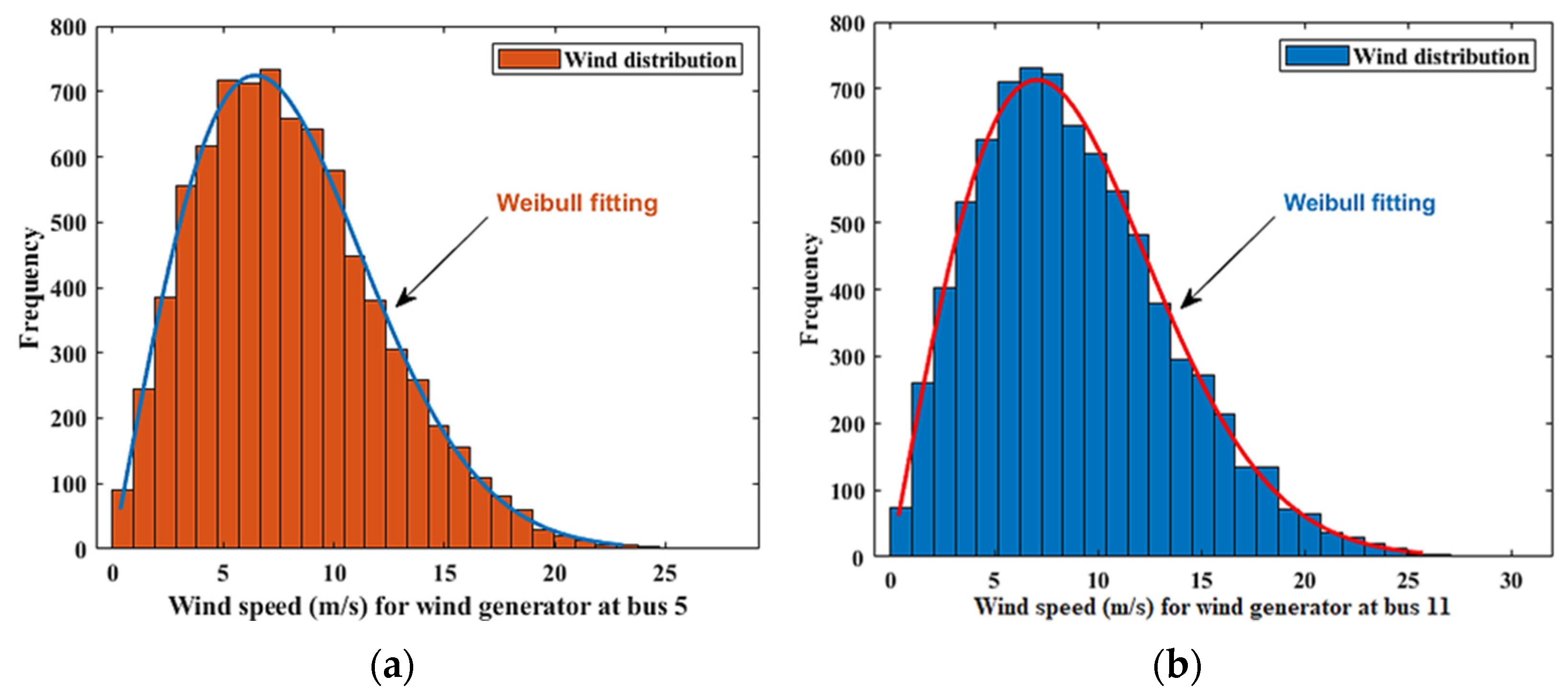
In this paper, as shown in Figure 1, the IEEE system with 30 buses has been updated by changing two thermal generators on buses 5 and 11 with two wind turbine generators, as well as replacing thermal generators at bus 13 with Solar PV. Table 3 shows the settings for the Weibull scale (c) and shape (k) variables that are used. Figure 2 shows the results of the Weibull fitting for wind frequency distributions. They were obtained by an 8000-iteration Monte Carlo simulation [16].
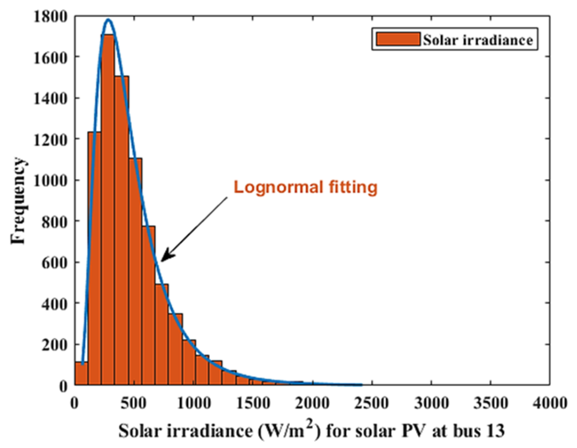
The output of a photovoltaic generator is determined by sun irradiation (R); it has a log-normal probability distributer (PDF) [32]. The probability of sun irradiation (R) is provided by the following log-normal PDF:
3.2. Power Models for Wind Generator and Solar Photovoltaic
The new IEEE-30 bus power system has two WPGs, as previously described in Figure 1. WPG1 is connected to bus 5 and has a total active power of 75 megawatts. WPG2 is connected to bus no. 11 and has a total power of 60 MW. The relationship between output power and wind speed is expressed as:
vr = rated speed, vout = cut-out speed, vin = cut-in speed of the wind turbine. Pwr = rated output power according to the product datasheet for (Enercon E82-E4) wind turbine. The generation of solar PV energy is measured in terms of solar radiation (R) [33].
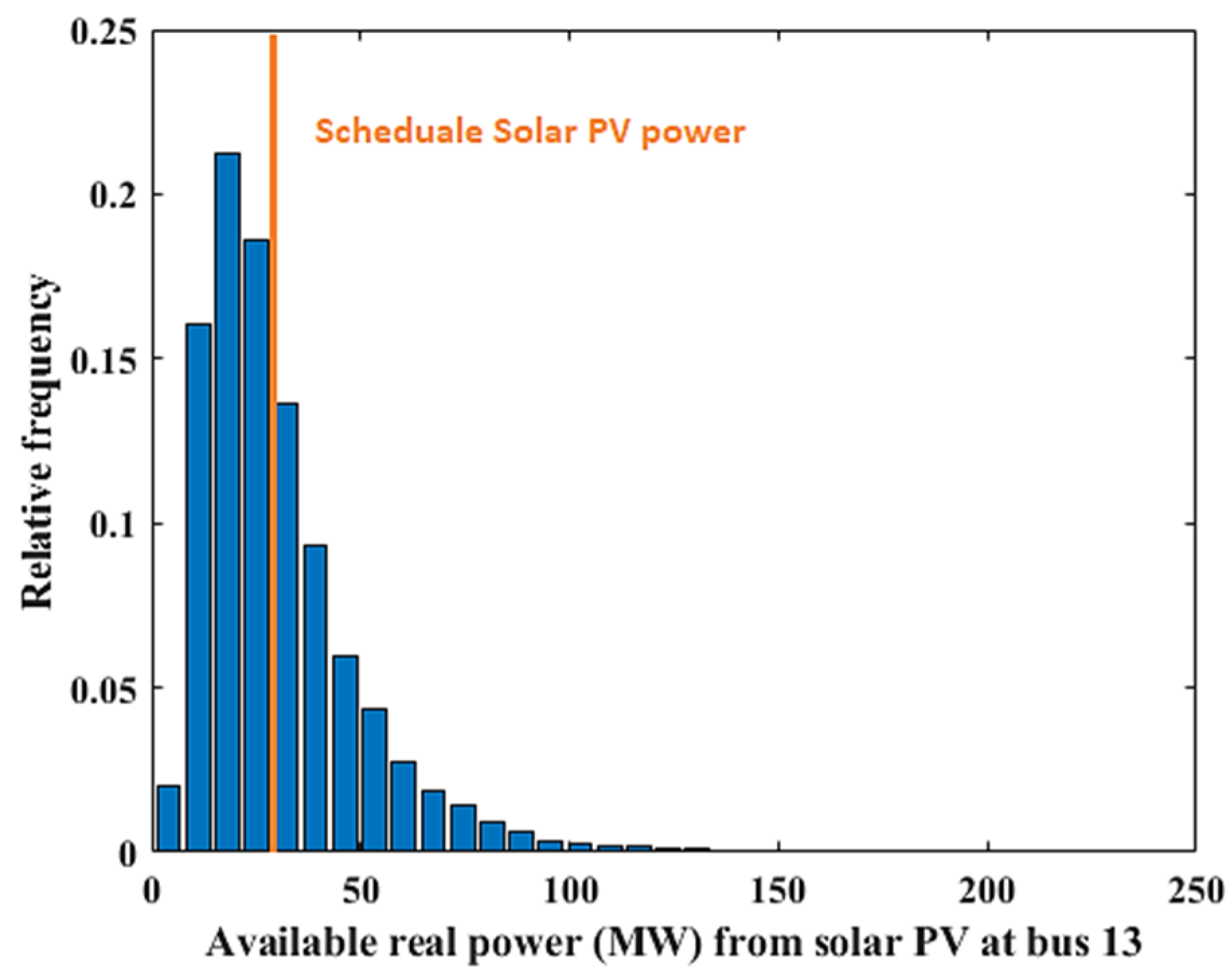
The histogram in Figure 4 represents the solar PV plant’s stochastic output power. The line depicts the planned power that the solar generator is meant to send to the network. It is important to remember that planned production solar power is a changeable value.
As a result, the ISO and the developer of the solar photovoltaic plant have entered into a power sharing arrangement.
Equations (36) and (37) are utilized in the model to calculate the overvaluation and undervaluation costs of solar PV electricity, respectively:
The shortfall and excess power are represented by PSn and PSn+, respectively.
4. The Basis of the Proposed Method’s Development
This study introduces the white shark optimizer (WSO), which is a new optimization algorithm inspired by white sharks’ scholastic behaviors when hunting in the wild to assist them in the ocean depths. The authors in [25] developed this algorithm within aim to solve real-world optimization problems that are difficult to solve using current techniques, both limited and unrestricted.
Many types of problems demand more flexibility than WSO can supply; hence, the suggested WSO provides several benefits for complex optimization problems, including its predicted adaptability in dealing with various types of optimization problems.
WSO’s mathematical approach makes it applicable to a wide range of engineering optimization problems, particularly those with high dimensionality. Its simplicity and resilience should allow it to identify the global optimum problems to challenging optimization problems quickly and precisely [25].
4.1. White Shark Optimizer (WSO)
The mathematical models of the proposed WSO to solve the OPF problem, which were built to define the actions of white sharks when hunting, are detailed in this section. This involves tracking and killing prey.
4.2. Initialization of WSO
As shown in the following 2d matrix, a population of n WSO, in a d search domain space, with the location of every shark indicating a suggested solution to these problems [25].
where w represents the location of all sharks in the search domain, d denotes the number of choice variables for a given task.
4.3. Speed of Movement towards Prey
A white shark recognizes a prey’s location by hearing a pause in the waves as the prey moves, as illustrated in Equation (39).
i = 1, 2, ……, n = index of size n, and the new speed vector of the ith shark is denoted by vik+1. vi is the ith index vector of sharks attaining the optimal location, as indicated by Equation (40).
where rand (1, n) = randomly generated numbers having a distribution in the domain [0, 1].
where k = current, K = maximum iterations, and pmin and pmax denote the starting and subordinate velocities for white shark motion. After a thorough examination, the values of pmin and pmax were discovered to be 0.5 and 1.5, respectively.
τ signifies the accelerating factor, which is 4.125, as was discovered after extensive research [25].
4.4. Movement in the Direction of the Optimal Prey
In this context, the position updating strategy defined in Equation (44) was used to describe the behavior of white sharks as they move towards prey.
Equations (45) and (46), respectively, define a and b as binary vectors.
where ⊕ is the result of a bitwise xor operation. The frequency of a white shark’s wavy motion and the multitude of times the shark attacks its target are described by Equations (48) and (49), respectively.
where a0 and a1 are location constants that are used for control exploration and exploitation.
4.5. Movement in the Direction of the Optimal Shark
Sharks can keep their place in front of the most advantageous one who is near to the target. Equation (50) shows how this phenomenon is expressed.
= upgraded shark’s location, sgn(r2 − 0.5) returns 1 or −1 to modify the search path, r1, r2, and r3 = rand. No. in the domain of [0, 1], Dw = length for both target and shark, is given in Equation (51). Ss is a parameter that has been proposed to reflect the power of white sharks, as specified in Equation (52).
where a2 is a location factor used to regulate exploration and exploitation.
Algorithm 1, the pseudo code of WSO [25].
| Algorithm 1: Code summarizing the iterative optimization process of WSO. | |
| 1: | Initialize the parameters of the problem |
| 2: | Initialize the parameters of WSO |
| 3: | Randomly generate the initial positions of WSO |
| 4: | Initialize the velocity of the initial population |
| 5: | Evaluate the position of the initial population |
| 6: | while (k < K) do |
| 7: | Update the parameters ν, p1, p2, µ, a, b, w0, f, mv and Ss using Equations (40)–(43), (45)–(49) and (52), respectively. |
| 8: | fori = 1 to n do |
| 9: | vik+1= µ [vik + p1 (wgbestk − wik) × c1 + p2(w′vkbest − wik) × c2] |
| 10: | end for |
| 11: | fori = 1 to n do |
| 12: | if rand < mv then |
| 13: | wik+1 = wik·− ⊕ w0 + u·a + l·b |
| 14: | else |
| 15: | wik+1 = wik + vik/f |
| 16: | end if |
| 17: | end for |
| 18: | fori = 1 to n do |
| 19: | if rand ≤ Ss then |
| 20: | |
| 21: | if i == 1 then |
| 22: | |
| 23: | else |
| 24: | |
| 25: | |
| 26: | end if |
| 27: | end if |
| 28: | end for |
| 29: | Adjust the position of the white sharks that proceed beyond the boundary |
| 30: | Evaluate and update the new positions |
| 31: | k = k + 1 |
| 32: | end while |
| 33: | Return the optimal solution obtained so far |
4.6. Fish School Behavior
The following formula was presented to define white shark fish school behavior:
where rand denotes a uniformly distributed random number in the range [0, 1]. As proven by Equation (52), the sharks are able to adjust their location based on the optimal shark who has arrived at the optimal location, which is very near to target. The end location of sharks is someplace ideally around the prey in the search space. The collective behavior of WSO is identified by fish action and the movement of sharks to the greatest shark, and improved local and global search capabilities.
4.7. Implementation and Analysis of WSO
During the process of function evaluations, white sharks always aim to move closer to the globally optimum solution. The reason is that white sharks are more likely to find a best answer by exploring and utilizing the search space’s surroundings. The location of the optimal sharks and their target is used to accomplish this ability. As a result, sharks are can constantly investigate and contribute to potentially prey-rich locations. The major steps of the algorithm in Algorithm 1 can be used to summaries the pseudo code of WSO.
WSO starts the optimization process by creating white shark positions at random, according to the algorithm in Algorithm 1. At each function execution, Equation (44) has been used to update the location of white sharks. WSO’s simulated steps will return them to the search region if they pass outside of the search space. To discover the white shark with the best fit value, a fitness process is used to estimate the optimal solution, with the fitness criterion being regenerated for every process estimation. The best stance for a white shark hunting prey is said to be the most suited solution [25].
5. Simulation Results and Comparison
In this section, the upgraded IEEE-30 bus power system is studied to find the optimal solution for the PF problem. The results of using the WSO to reduce the total power generation cost are provided and explained. Northern Goshawk Optimizer (NGO) and two alternative optimization algorithms, SAO and POA, are also applied to verify the validity of WSO. The optimization algorithms are simulated using MATLAB (2018b) on a computer that has the following specifications: Intel® Core(TM) i5-3210M processor, 2.5 GHz, and 8 GB of RAM.
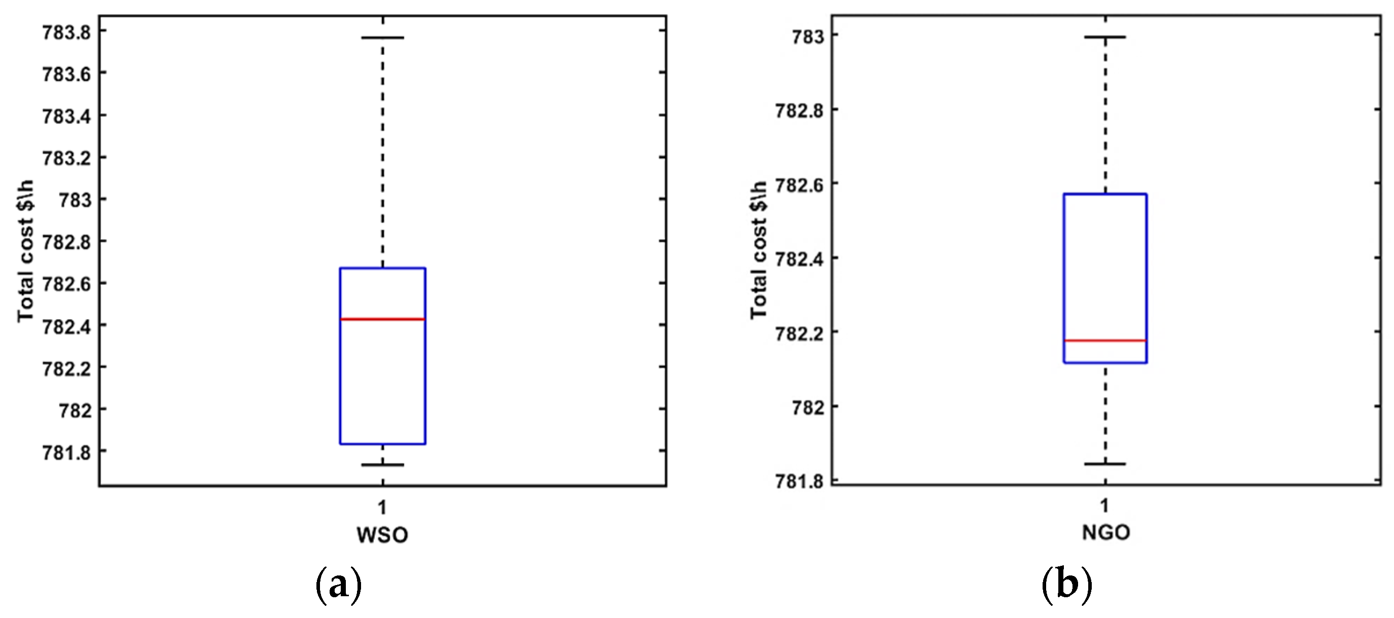
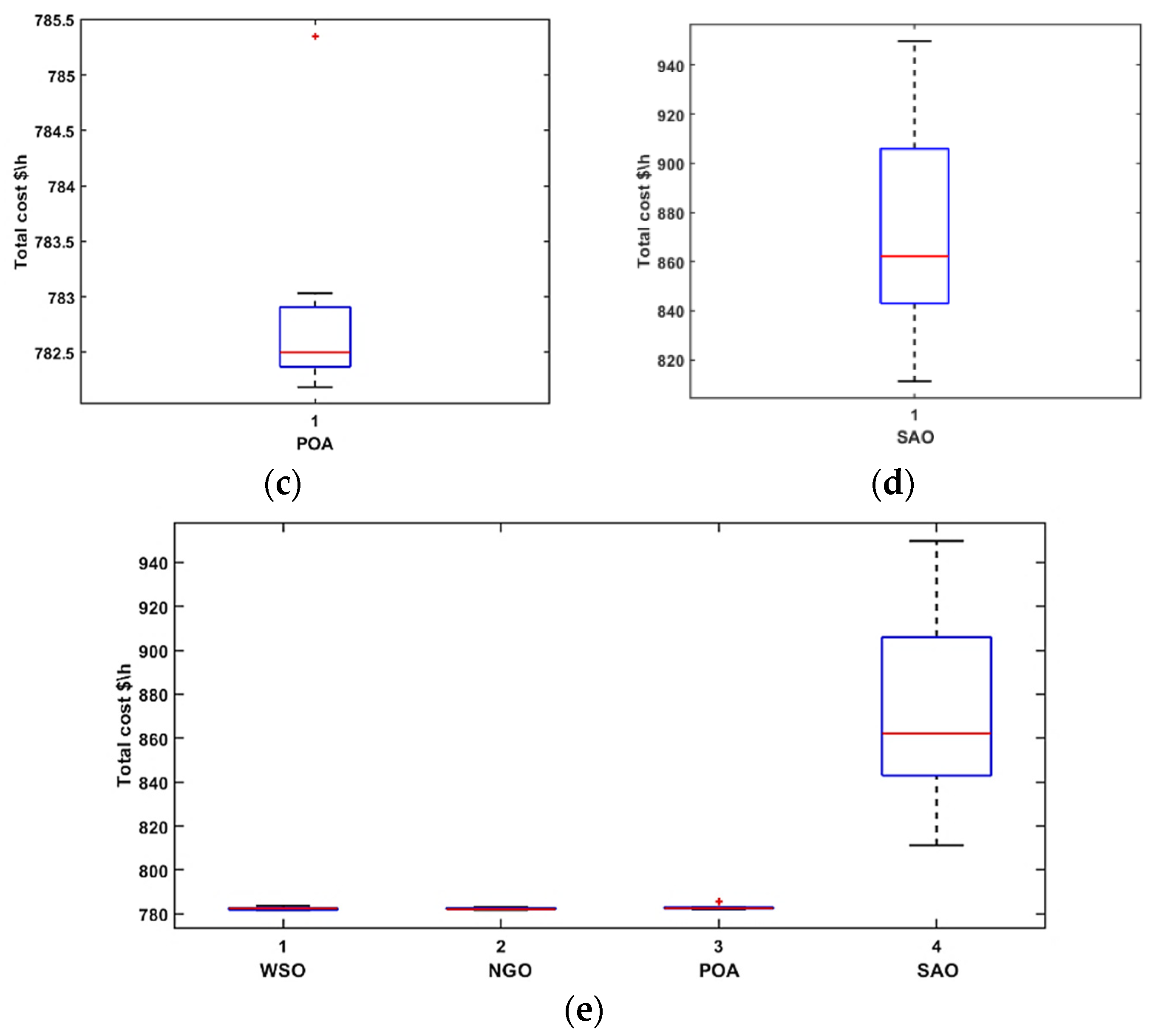
The four algorithms were prepared to find the optimal solution after 10 runs and 300 iterations. The statistical results in Table 4 show that WSO and NGO’s values are always close to the optimal solution, with a standard deviation of 0.6722 and 0.3766, respectively. However, WSO is the best of the four in terms of convergence time, with an average of 524 s for one run. Figure 5 shows the boxplots for distributing the statistics of the results to all the methods, it’s clear that the boxplots of the WSO technique are narrow compared to the other techniques, where POA in Figure 5c contains one suspected outlier.
The best three solutions were selected among the ten to be presented in the results and to study the convergence for each case in terms of reaching the lowest value of the total power generation cost by finding the optimal solution for scheduling and using power from different power plants according to Equation (15). The simulation results for all four algorithms were as follows:
5.1. White Shark Optimizer (WSO)
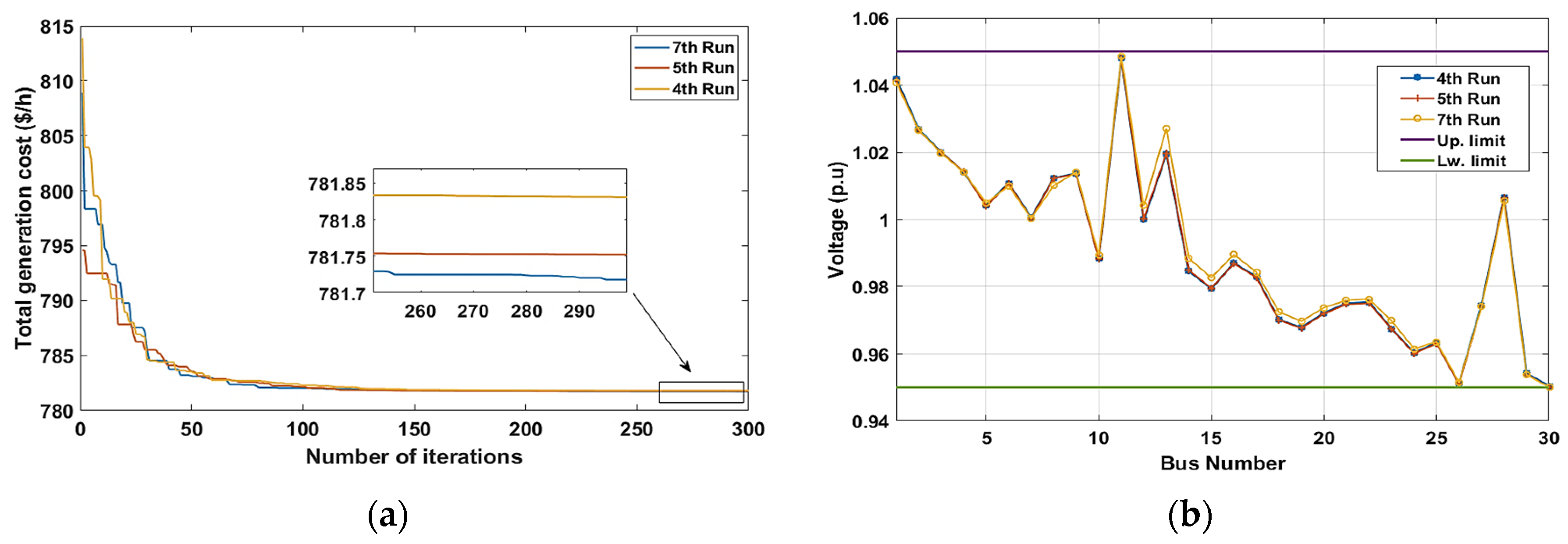
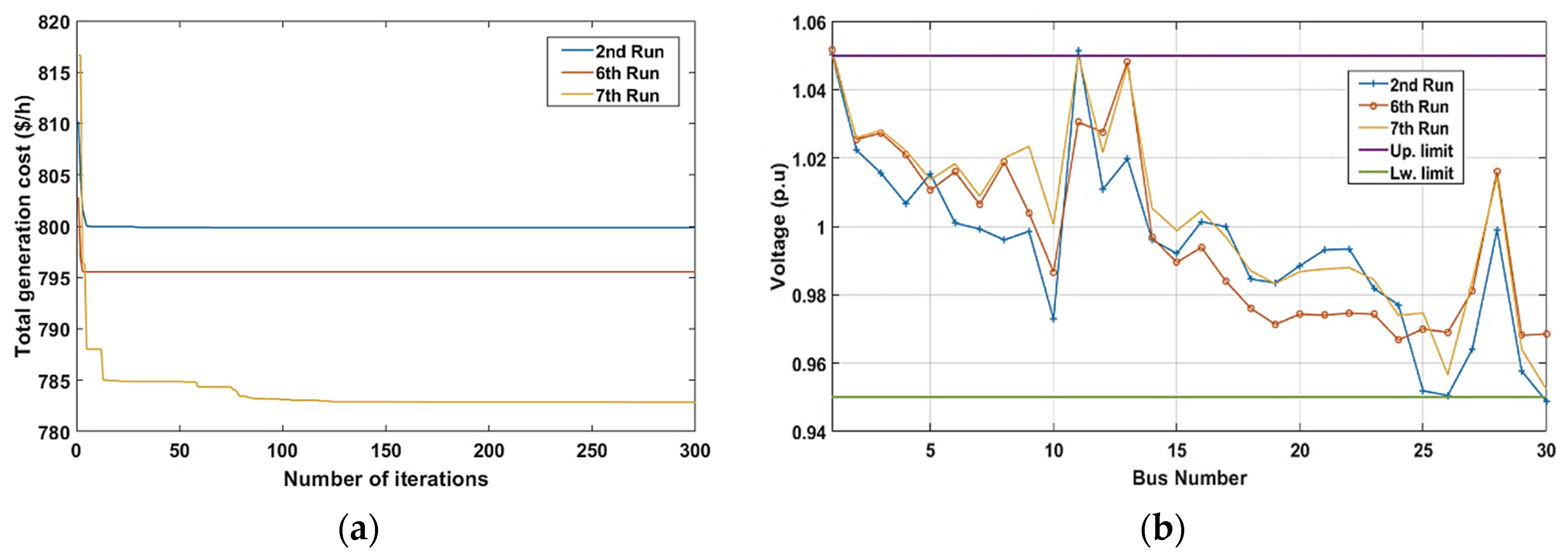
The white shark optimizer (WSO) was implemented and used to obtain an optimal solution to the problem of scheduling the generation power to minimize the total generation cost by performing 10 runs each time with 300 iterations. Among all 10 runs, three were given preference: the seventh, the fifth, and the fourth, achieving a generation cost of 781.733, 781.755, and 781.831 USD/h, respectively, as shown in Figure 6a. Thus, the seventh run was chosen to be the best performer at the lowest total generating cost of 781.733 USD/h.
The voltages of the load buses play a significant part in the OPF investigation. As a result, dealing with the voltage constraints of load buses is critical. The buses of load in the IEEE system with 30 buses must have voltages between [0.95: 1.05] p.u. Where Figure 6b shows the voltage levels in the load buses for the best three runs of WSO. It is obvious from the figure that all voltages for the load buses fall within the safe limits for operation.
5.2. Northern Goshawk Optimization (NGO)
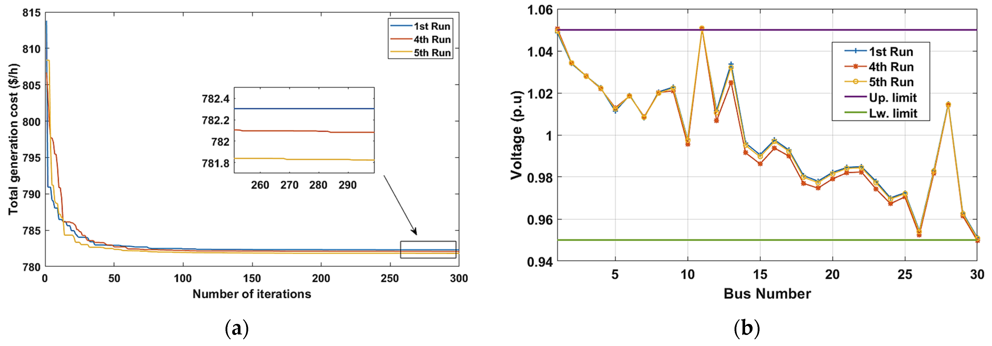
As the same in WSO, the NGO was implemented to minimize the total generation cost by doing 10 runs each time with 300 iterations. Among of all 10 runs, three were given preference: the fifth, the fourth, and the first, achieving a generation cost of 781.843, 782.124, and 782.313 USD/h, respectively, as shown in Figure 7a. Thus, the fifth run was chosen to be the best performer at the lowest total generating cost of 781.843 USD/h. Figure 7b provides load bus voltage characteristics for the best three runs of NGO. It is obvious from the figure that all voltages for the load buses fall within the safe limits for operation.
5.3. Pelican Optimization Algorithm (POA)
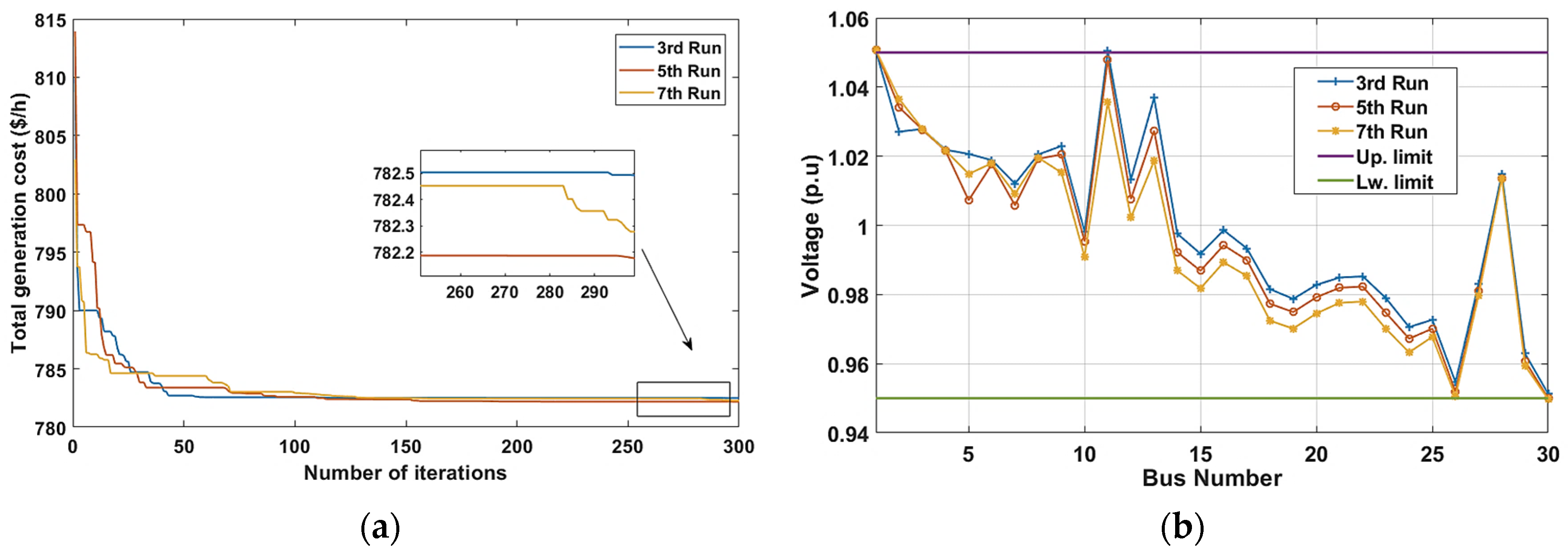
As the same in WSO and NGO, the POA was implemented to minimize the total generation cost by doing 10 runs each time with 300 iterations. Among of all 10 runs, three were given preference: the fifth, seventh and third, achieving a generation cost of 782.186, 782.299, and 782.508 USD/h, respectively, as shown in Figure 8a. Thus, the fifth run was chosen to be the best performer at the lowest total generating cost of 782.186 USD/h. Figure 8b provides load bus voltage characteristics for the best three runs of POA.
It is obvious from the figure that all voltages for the load buses fall within the safe limits for operation.
5.4. Smell Agent Optimization (SAO)
As in the previous cases, the SAO was implemented to minimize the total generation cost by doing 10 runs each time with 300 iterations. Among of all 10 runs, three were given preference: the seventh, sixth and second, achieving a generation cost of 811.187, 851.711, and 846.683 $/h, respectively, as shown in Figure 9a. Thus, the seventh run was chosen to be the best performer at the lowest total generating cost of 811.187 USD/h. Figure 9b provides load bus voltage characteristics for the best three runs of SAO. It is obvious from the figure that all voltages for the load buses almost fall within the safe limits for operation.
5.5. Comparison of the Results of Different Optimization Techniques and Discussion
In this section, the results of WHO and the other three algorithms mentioned above, in addition to ESMAOPF in [18], have been compared to verify the validity of WSO to optimize schedule power generation from all power plants connected to the upgraded system in order to achieve the minimum total power cost. Table 5 records optimal schedule power and overall generation cost for all algorithms including ESMA [18], reactive power (Q), control variables, and other essential estimated values.
The convergence curves of the various (OPF) optimizer applications applied in this investigation are illustrated in Figure 10. The success and effectiveness of the algorithm (WSO) among the rest of the others in reaching the optimal solution for scheduling the generated power and reducing the total generation cost is clear from the results in this figure.
It is clear from zooming in on the convergence curves that the curve of WSO reached its lowest value between the 290 and 300 iteration and achieved the lowest cost of 781.733 USD/h. While the algorithm NGO achieved a total generation cost of 781.844 USD/h, followed by the algorithm POA at a cost of 782.186 %/h; finally, SAO achieved a cost of 811.187 USD/h. Moreover, by comparing the results of the total generation cost presented in Table 5, it becomes clear that the efficiency of the algorithm WSO is better than ESMA, which the authors used in [18], and in which it achieved a cost of 791.937 USD/h, while both WSO and NGO achieved a lower cost.
The effectiveness of WSO can be shown in the simulation results when compared to ESMA in [18] and other optimization techniques used for NGO, POA, and SAO. As a result, the suggested method has a higher solution quality and several advantages, including easier application, fewer control parameters, less time spent adjusting control parameter values, faster convergence to optimal solutions, and more steady search capabilities.
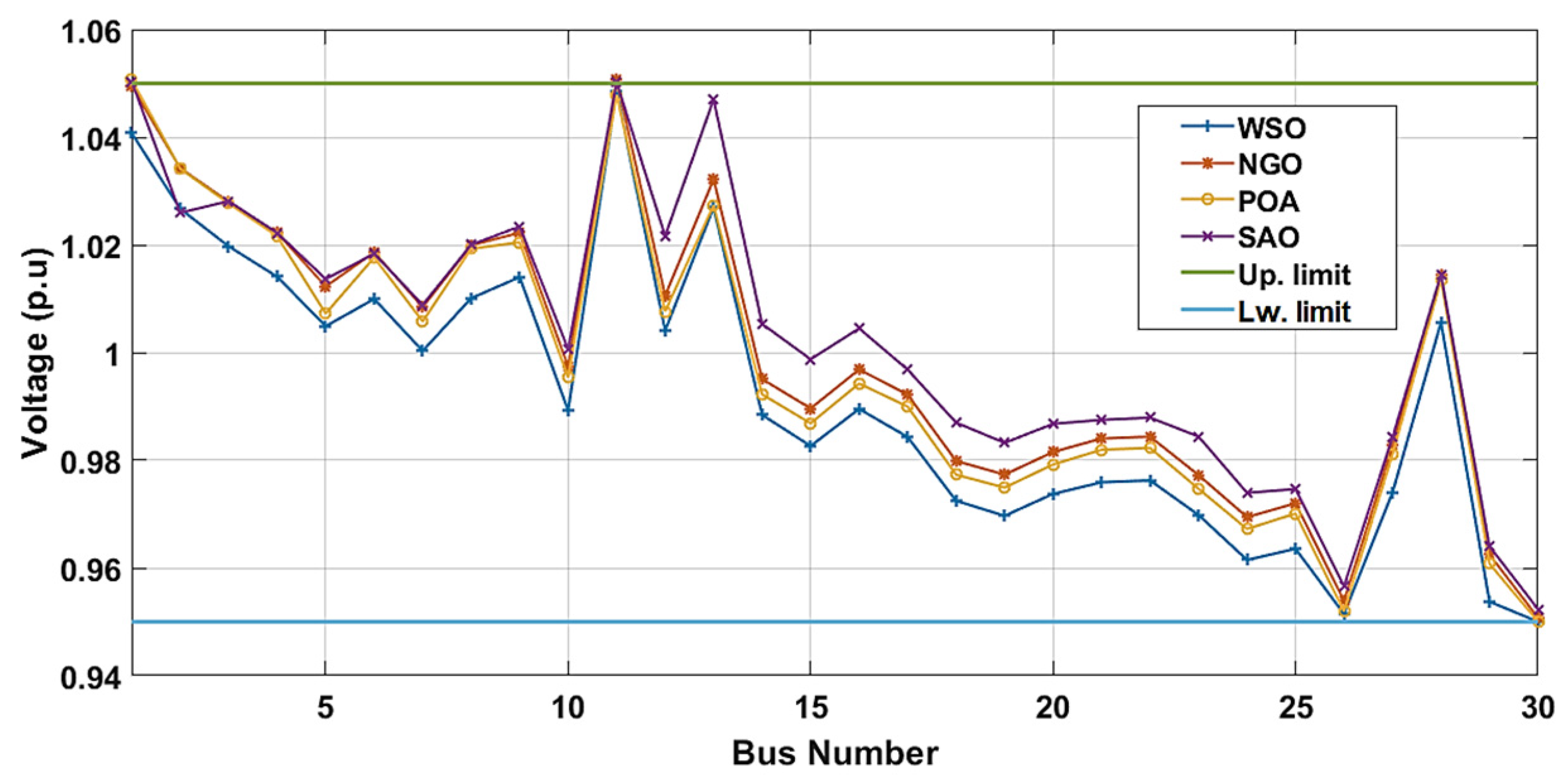
Table 5 also shows the bus voltage values for the generation buses, which are six buses. Figure 11 shows the voltage values for all buses of loads for all the applications of the previously mentioned optimization algorithms. It becomes clear that most of the efforts are within the acceptable limits.
Figure 12 shows the results of all optimization algorithms for optimizing the power cost of thermal, wind, and solar power plants. The lack of output power from wind and solar PV sources is compensated by thermal power generators. As a result, the cost of a thermal power generation system rises, as shown in the cost characteristic of a thermal power source (TPG) in Figure 12, whereas the cost of WPG and SPG steadily reduces to a certain level.
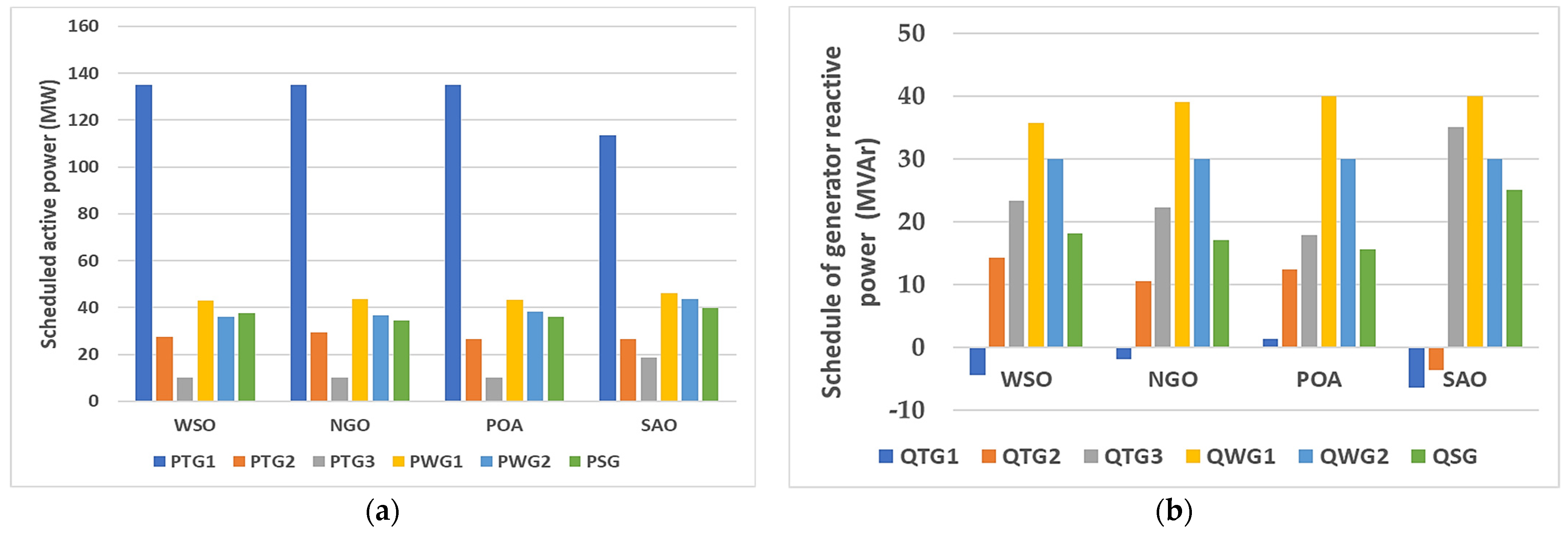
Figure 13a depicts the optimal results of the planned powers of thermal, wind, and solar power generators. When sun irradiation or wind speed are great, ideal planned power from wind and solar PV facilities improves because raising the planned produced power helps to minimize the penalization cost. The planned reactive power from all power plants is depicted in Figure 13b. In several cases, the generators TG3 and WG2 run at their maximum reactive power (Q) capability by following the constraints of reactive power (Q), as indicated in Table 5. As a result, whenever an optimization technique is implemented, the limitations on Q must be considered.
6. Conclusions
In this study, a novel meta-heuristic optimization algorithm, so called the white shark optimizer (WSO), has been proposed for providing an optimal solution for the OPF problem in the IEEE-30 bus power system which has been upgraded with unpredictable wind and solar photovoltaic energy sources. Weibull and lognormal probability density functions (PDFs) were used to describe the uncertain outputs of wind and solar energy sources, respectively. The WSO and another three optimization algorithms have been used to optimize the scheduling of power generation with both traditional thermal power plants and renewable power sources to minimize the total electricity generation cost. To verify the WSO performance, the results of the proposed algorithm has been compared with the results obtained from the other three optimizers (NGO, POA, and SAO).
The results showed the effectiveness of the WSO algorithm in solving the OPF problem and in achieving the minimum total generation cost (781.733 USD/h) among the other three algorithms and ESMA, where the overall power produced cost from all power plants was optimally minimized. Moreover, the results of WSO and the other three application algorithms also reveal that the environmental and safety constraints are in the system operator’s stated boundaries. In addition, the results were compared with the ESMA method that the authors used in [18], and the comparison showed the success of WSO over ESMAOPF in terms of achieving a lower total generating cost.
As a result, the algorithm has advantages over ESMA and the other three proposed algorithms in this paper, such as simpler application, fewer control parameters, less time spent tuning control parameter values, faster convergence to optimal solutions, fewer generated new solutions, shorter simulation time, and more stable search ability. Therefore, we can conclude that WSO is a powerful method for dealing with optimal power flow problems where optimization of single objectives is required.
7. Future Work
- Apply the proposed methods to solve optimal power flow in a larger power system;
- Incorporate more renewable energy sources (such as hydropower plants) into the larger power system;
- Apply of more than one case study that takes into account factors other than the minimization of generation cost, such as emissions, carbon tax, reserve cost, penalty cost, and the dynamic nature of generating facilities’ control;
- Studying multi-objective optimal power flow in a power system with renewable energy sources.
Author Contributions
Conceptualization, S.K., M.H.H. and E.M.A.; Data curation, M.A.A. and M.H.H.; Formal analysis, M.A.A. and S.K.; Funding acquisition, S.K., E.M.A. and M.A.; Investigation, M.A.A. and S.K.; Methodology, M.A.A., S.K., M.H.H., E.M.A. and M.A.; Project administration, S.K. and E.M.A.; Resources, M.H.H. and M.A.; Software, M.A.A. and E.M.A.; Validation, S.K., M.H.H., E.M.A. and M.A.; Writing—original draft, M.A.A. and M.H.H.; Writing—review & editing, S.K., E.M.A. and M.A. All authors have read and agreed to the published version of the manuscript.
Funding
This research received no external funding.
Institutional Review Board Statement
Not applicable.
Informed Consent Statement
Not applicable.
Data Availability Statement
Not applicable.
Conflicts of Interest
The authors declare no conflict of interest.
References
- Farhat, M.; Kamel, S.; Atallah, A.M.; Khan, B. Optimal Power Flow Solution Based on Jellyfish Search Optimization Considering Uncertainty of Renewable Energy Sources. IEEE Access 2021, 9, 100911–100933. Available online: https://ieeexplore.ieee.org/document/9481886 (accessed on 22 July 2021). [CrossRef]
- Carpentier, J. Contribution to the economic dispatch problem. Bull. Soc. Fr. Electr. 1962, 3, 431–447. [Google Scholar]
- Nguyen, T.T. A high performance social spider optimization algorithm for optimal power flow solution with single objective optimization. Energy 2019, 171, 218–240. [Google Scholar] [CrossRef]
- Momoh, J.A.; Adapa, R.; El-Hawary, M.E. A review of selected optimal power flow literature to 1993. I. Nonlinear and quadratic programming approaches. IEEE Trans. Power Syst. 1993, 14, 96–104. [Google Scholar]
- Roy, R.; Jadhav, H.T. Optimal power flow solution of power system incorporating stochastic wind power using Gbest guided artificial bee colony algorithm. Int. J. Electr. Power Energy Syst. 2015, 64, 562–578. [Google Scholar] [CrossRef]
- Panda, A.; Tripathy, M. Security constrained optimal power flow solution of wind-thermal generation system using modified bacteria foraging algorithm. Energy 2015, 93, 816–827. [Google Scholar] [CrossRef]
- Ravi, K. Optimal power flow considering intermittent wind power using particle swarm optimization. Int. J. Renew. Energy Res. 2016, 6, 504–509. [Google Scholar]
- Abido, M.A. Optimal power flow using tabu search algorithm. Electr. Power Compon. Syst. 2002, 30, 469–483. [Google Scholar] [CrossRef] [Green Version]
- Niknam, T.; Narimani, M.R.; Aghaei, J.; Tabatabaei, S.; Nayeripour, M. Modified honeybee mating optimisation to solve dynamic optimal power flow considering generator constraints. IET Gener. Transm. Distrib. 2011, 5, 989–1002. [Google Scholar] [CrossRef]
- Ara, A.L.; Kazemi, A.; Gahramani, S.; Behshad, M. Optimal reactive power flow using multi-objective mathematical programming. Sci. Iran. 2012, 19, 1829–1836. [Google Scholar]
- Duman, S.; Güvenç, U.; Sonmez, Y.; Yörükeren, N. Optimal power flow using gravitational search algorithm. Energy Convers. Manag. 2012, 59, 86–95. [Google Scholar] [CrossRef]
- Adaryani, M.R.; Karami, A. Artificial bee colony algorithm for solving multiobjective optimal power flow problem. Int. J. Electr. Power Energy Syst. 2013, 53, 219–230. [Google Scholar] [CrossRef]
- Ghasemi, M.; Ghavidel, S.; Ghanbarian, M.M.; Gharibzadeh, M.; Vahed, A.A. Multiobjective optimal power flow considering the cost, emission, voltage deviation and power losses using multi-objective modified imperialist competitive algorithm. Energy 2014, 78, 276–289. [Google Scholar] [CrossRef]
- Le Anh, T.N.; Vo, D.N.; Ongsakul, W.; Vasant, P.; Ganesan, T. Cuckoo optimization algorithm for optimal power flow. In Proceedings of the 18th Asia Pacific Symposium on Intelligent and Evolutionary Systems, Singapore, 10–12 November 2014; Volume 479, p. 4931. [Google Scholar]
- Ladumor, D.P.; Trivedi, I.N.; Bhesdadiya, R.H.; Jangir, P. A grey wolf optimizer algorithm for voltage stability enhancement. In Proceedings of the Third International Conference on Advances in Electrical, Electronics, Information, Communication and Bio-Informatics (AEEICB), Chennai, India, 27–28 February 2017; pp. 278–282. [Google Scholar]
- Biswas, P.P.; Suganthan, P.N.; Amaratunga, G.A. Optimal power flow solutions incorporating stochastic wind and solar power. Energy Convers. Manag. 2017, 148, 1194–1207. [Google Scholar] [CrossRef]
- Khan, B.; Singh, P. Optimal power flow techniques under characterization of conventional and renewable energy sources: A comprehensive analysis. J. Eng. 2017, 2017, 9539506. [Google Scholar] [CrossRef] [Green Version]
- Farhat, M.; Kamel, S.; Atallah, A.M.; Hassan, M.H.; Agwa, A.M. ESMA-OPF: Enhanced Slime Mould Algorithm for Solving Optimal Power Flow Problem. Sustainability 2022, 14, 2305. [Google Scholar] [CrossRef]
- Ghasemi, M.; Ghavidel, S.; Ghanbarian, M.M.; Gitizadeh, M. Multi-objective optimal electric power planning in the power system using Gaussian barebones imperialist competitive algorithm. Inf. Sci. 2015, 294, 286–304. [Google Scholar]
- El-Hana Bouchekara, H.R.; Abido, M.A.; Chaib, A.E. Optimal power flow using an improved electromagnetism-like mechanism method. Electr. Power Compon. Syst. 2016, 44, 434–449. [Google Scholar] [CrossRef]
- Bouchekara, H.R.E.H.; Chaib, A.E.; Abido, M.A.; El-Sehiemy, R.A. Optimal power flow using an improved colliding Bodies optimization algorithm. Appl. Soft Comput. 2016, 42, 119–131. [Google Scholar] [CrossRef]
- Abaci, K.; Yamacli, V. Differential search algorithm for solving multi-objective optimal power flow problem. Int. J. Electr. Power Energy Syst. 2016, 1, 10–79. [Google Scholar] [CrossRef]
- Pulluri, H.; Naresh, R.; Sharma, V. A solution network based on stud krill herd algorithm for optimal power flow problems. Soft Comput. 2018, 22, 159–176. [Google Scholar] [CrossRef]
- Niknam, T.; Rasoul Narimani, M.; Jabbari, M.; Malekpour, A.R. A modified shuffle frog leaping algorithm for multi-objective optimal power flow. Energy 2011, 36, 6420–6432. [Google Scholar] [CrossRef]
- Braik, M.; Hammouri, A.; Atwan, J.; Al-Betar, M.A.; Awadallah, M.A. White Shark Optimizer: A novel bio-inspired meta-heuristic algorithm for global optimization problems. Knowl. Based Syst. 2022, 243, 108457. Available online: www.elsevier.com/locate/knosys (accessed on 22 February 2022). [CrossRef]
- Salawudeen, A.T.; Mu’azu, M.B.; Sha’aban, Y.A.; Adedokun, E.A. A Novel Smell Agent Optimization: An Extensive CEC Study and Engineering Application. Knowl. Based Syst. 2021, 232, 107486. [Google Scholar] [CrossRef]
- Dehghani, M.; Hubálovský, Š.; Trojovský, P. Northern Goshawk Optimization: A New Swarm-Based Algorithm for Solving Optimization Problems. IEEE Access 2021, 9, 162059–162080. [Google Scholar] [CrossRef]
- Trojovský, P.; Dehghani, M. Pelican Optimization Algorithm: A Novel Nature-Inspired Algorithm for Engineering Applications. Sensors 2022, 22, 855. [Google Scholar] [CrossRef]
- Alsac, O.; Stott, B. Optimal load flow with steady-state security. IEEE Trans. Power Appar. Syst. 1974, 93, 745–751. [Google Scholar] [CrossRef] [Green Version]
- Chaib, A.E.; Bouchekara, H.R.; Mehasni, R.; Abido, M.A. Optimal power flow with emission and non-smooth cost functions using backtracking search optimization algorithm. Int. J. Electr. Power Energy Syst. 2016, 81, 64–77. [Google Scholar] [CrossRef]
- Shi, L.; Wang, C.; Yao, L.; Ni, Y.; Bazargan, M. Optimal power flow solution incorporating wind power. IEEE Syst. J. 2012, 6, 233–241. [Google Scholar] [CrossRef]
- Tian-Pau, C. Investigation on frequency distribution of global radiation using different probability density functions. Int. J. Appl. Sci. Eng. 2010, 8, 99–107. [Google Scholar]
- Reddy, S.S.; Bijwe, P.R.; Abhyankar, A.R. Real-time economic dispatch considering renewable power generation variability and uncertainty over scheduling period. IEEE Syst. J. 2014, 9, 1440–1451. [Google Scholar] [CrossRef]
Figure 1.
Upgraded IEEE-30 bus power system.

Figure 2.
The Weibull PDF Distribution for wind speed: (a) WPG1, bus 5, and (b) WPG2, bus 11.

Figure 3.
The lognormal PDF solar irradiance distribution for solar PV generator at bus 13.

Figure 4.
Available power distribution of solar PV (MW) at bus 13.

Figure 5.
The boxplots for all algorithms for the statistical results: (a) boxplot for WSO, (b) boxplot for NGO, (c) boxplot for POA (red + = suspected outliers), (d) boxplot for SAO, (e) boxplots for all.
Figure 5.
The boxplots for all algorithms for the statistical results: (a) boxplot for WSO, (b) boxplot for NGO, (c) boxplot for POA (red + = suspected outliers), (d) boxplot for SAO, (e) boxplots for all.


Figure 6.
The WSO results for the best 3 runs: (a) characteristics of convergence for the best three runs of WSO algorithm; (b) profile voltages of load buses for the best three runs of WSO.
Figure 6.
The WSO results for the best 3 runs: (a) characteristics of convergence for the best three runs of WSO algorithm; (b) profile voltages of load buses for the best three runs of WSO.

Figure 7.
The NGO results for the best 3 runs: (a) characteristics of convergence for the best three runs of NGO algorithm; (b) profile voltages of load buses for the best three runs of NGO.
Figure 7.
The NGO results for the best 3 runs: (a) characteristics of convergence for the best three runs of NGO algorithm; (b) profile voltages of load buses for the best three runs of NGO.

Figure 8.
The POA results for the best 3 runs: (a) characteristics of convergence for the best three runs of POA algorithm; (b) profile voltages of load buses for the best three runs of POA.
Figure 8.
The POA results for the best 3 runs: (a) characteristics of convergence for the best three runs of POA algorithm; (b) profile voltages of load buses for the best three runs of POA.

Figure 9.
The SAO results for the best 3 runs: (a) characteristics of convergence for the best three runs of SAO algorithm; (b) profile voltages of Load buses for the best three runs of SAO.
Figure 9.
The SAO results for the best 3 runs: (a) characteristics of convergence for the best three runs of SAO algorithm; (b) profile voltages of Load buses for the best three runs of SAO.

Figure 10.
Convergence curves for various optimization applications.

Figure 11.
Load buses’ voltages for the different optimization algorithms.

Figure 12.
Costs variation of all generators for all algorithms.

Figure 13.
The optimal scheduled active and reactive power for different optimization techniques: (a) optimal scheduled active power (MW) with different optimization techniques; (b) optimal scheduled reactive power (MVAr) with different optimization techniques.
Figure 13.
The optimal scheduled active and reactive power for different optimization techniques: (a) optimal scheduled active power (MW) with different optimization techniques; (b) optimal scheduled reactive power (MVAr) with different optimization techniques.


Table 1.
The basic specifications of the modified IEEE network with 30 buses [1].
Table 1.
The basic specifications of the modified IEEE network with 30 buses [1].
| Items | Quantity | Details |
|---|---|---|
| Buses | 30 | [29] |
| Branches | 41 | [29] |
| Thermal Generators (TG1, TG2, TG3) | 3 | Bus 1 (Swing), Bus 2, and Bus 8. |
| Wind Generators (WPG1, WPG2) | 2 | Bus 5 and bus 11. |
| Solar PV (SPG) | 1 | Bus 13. |
| Control variables | 11 | The planned power of five generators (TG2, TG3, WPG1, WPG2, and SPG), as well as six generating bus voltages. |
| Connected load | - | 283.4 MW, 126.2 MVAR |
| Allowable voltage range for load buses | 24 | [0.95–1.05] p.u. |
Table 2.
Cost and emission coefficients of thermal power generators [18].
Table 2.
Cost and emission coefficients of thermal power generators [18].
| Gen. | Bus | a | b | c | l | m | α | β | γ | ω | μ | P0TGi (MW) | DRi (MW) | URi (MW) |
|---|---|---|---|---|---|---|---|---|---|---|---|---|---|---|
| TG1 | 1 | 0 | 2 | 0.00375 | 18 | 0.037 | 4.091 | −5.554 | 6.49 | 0.0002 | 6.667 | 99.211 | 20 | 15 |
| TG2 | 2 | 0 | 1.75 | 0.0175 | 16 | 0.038 | 2.543 | −6.047 | 5.638 | 0.0005 | 3.333 | 80 | 15 | 10 |
| TG3 | 8 | 0 | 3.25 | 0.00834 | 12 | 0.045 | 5.326 | −3.55 | 3.38 | 0.002 | 2 | 20 | 8 | 4 |
Table 3.
The PDF parameters for wind and solar PV power plants.
| Wind Power Farm | Solar Power Plant | ||||||
|---|---|---|---|---|---|---|---|
| Wind Power Generator | No. of Turbines | Rated Power (MW) | Weibull PDF Parameters | Weibull Mean, Mwbl | Rated Power (MW) | Lognormal PDF Parameters | Lognormal |
| 1 (at bus 5) | 25 | 75 | K = 2, c = 9 | v = 7.976 (m/s) | 50 (at bus 13) | μ = 6, δ = 0.6 | R = 483 W/m2 |
| 2 (at bus 11) | 20 | 60 | K = 2, c = 10 | v = 8.862 (m/s) | |||
Table 4.
The results of total generation cost and statistical results for the proposed WSO algorithm and other recent algorithms.
Table 4.
The results of total generation cost and statistical results for the proposed WSO algorithm and other recent algorithms.
| The Results of Total Generation Cost for 10 Runs and 300 Iterations | ||||
| WSO | NGO | POA | SAO | |
| 1st Run | 782.6698 | 782.313 | 782.8485 | 907.0226 |
| 2nd Run | 783.7659 | 782.9944 | 785.3441 | 846.683 |
| 3rd Run | 782.5018 | 782.5711 | 782.5089 | 843.0099 |
| 4th Run | 781.8318 | 782.1243 | 782.4893 | 905.917 |
| 5th Run | 781.7552 | 781.8438 | 782.1865 | 872.6064 |
| 6th Run | 782.3621 | 782.2253 | 782.3702 | 851.711 |
| 7th Run | 781.733 | 782.9235 | 782.2994 | 811.187 |
| 8th Run | 783.3357 | 782.1109 | 782.4652 | 887.9602 |
| 9th Run | 782.4915 | 782.1162 | 782.9073 | 949.768 |
| 10th Run | 782.1152 | 782.1276 | 783.033 | 823.5738 |
| The Statistical Results of Total Generation Cost for 10 Runs and 300 Iterations | ||||
| WSO | NGO | POA | SAO | |
| Best | 781.733 | 781.8438 | 782.1865 | 811.187 |
| Worst | 783.7659 | 782.9944 | 785.3441 | 949.768 |
| Mean | 782.4562 | 782.335 | 782.8452 | 869.9439 |
| Std | 0.6722 | 0.3766 | 0.9205 | 42.9133 |
| Average time of one run (s) | 524 | 1024 | 1610 | 1790 |
Table 5.
Detail simulation results of the different optimization algorithms (in addition to ESMA).
| Control Variables | Min | Max | WSO | NGO | POA | SAO | ESMA [18] |
| PTG1 (MW) | 50 | 140 | 134.9165 | 134.9041 | 134.9076 | 113.404 | 134.9143 |
| PTG2 (MW) | 20 | 80 | 27.57455 | 29.36321 | 26.6666 | 26.64171 | 27.688 |
| PTG3 (MW) | 10 | 35 | 10.00492 | 10.0109 | 10.02834 | 18.70488 | 10.0125 |
| PwG1 (MW) | 0 | 75 | 43.05681 | 43.73514 | 43.27867 | 46.21081 | 43.5782 |
| PwG2 (MW) | 0 | 60 | 36.12732 | 36.71591 | 38.29961 | 43.67977 | 37.4508 |
| PsG1 (MW) | 0 | 50 | 37.52105 | 34.45914 | 35.97858 | 39.90458 | 35.5275 |
| V1 (p.u) | 0.95 | 1.1 | 1.070752 | 1.071513 | 1.072656 | 1.017665 | 1.0699 |
| V2 (p.u) | 0.95 | 1.1 | 1.056697 | 1.056241 | 1.056156 | 1.004626 | 1.0568 |
| V5 (p.u) | 0.95 | 1.1 | 1.034903 | 1.034296 | 1.029249 | 1.095148 | 1.0334 |
| V8 (p.u) | 0.95 | 1.1 | 1.0401 | 1.041903 | 1.043762 | 1.105398 | 1.088 |
| V11 (p.u) | 0.95 | 1.1 | 1.099687 | 1.099531 | 1.099998 | 1.084872 | 1.097 |
| V13 (p.u) | 0.95 | 1.1 | 1.056971 | 1.054164 | 1.049375 | 1.109471 | 1.052 |
| Parameters | Min | Max | WSO | NGO | POA | SAO | ESMA [18] |
| QTG1 (MVAr) | −20 | 150 | −4.43953 | −1.8199 | 1.326721 | −6.41329 | −6.588 |
| QTG2 (MVAr) | −20 | 60 | 14.28056 | 10.49797 | 12.42993 | −3.53766 | 16.436 |
| QTG3 (MVAr) | −15 | 40 | 23.31959 | 22.32038 | 17.85702 | 35 | 40 |
| QwG1 (MVAr) | −30 | 35 | 35.7025 | 39.00757 | 40 | 40 | 21.181 |
| QwG2 (MVAr) | −25 | 30 | 30 | 30 | 30 | 30 | 29.548 |
| QwG1 (MVAr) | −20 | 25 | 18.19068 | 17.01745 | 15.63321 | 25 | 16.472 |
| Total power cost (USD/h) | 781.733 | 781.8438 | 782.1865 | 811.1871 | 781.9375 | ||
| Emissions (t/h) | 1.763241 | 1.761466 | 1.7625 | 0.510854 | 1.7629 | ||
| Ploss (MW) | 5.80114 | 5.788415 | 5.759369 | 5.145789 | 5.7715 | ||
| Vd (p.u) | 0.468569 | 0.465172 | 0.44752 | 0.68291 | 0.45868 |
Publisher’s Note: MDPI stays neutral with regard to jurisdictional claims in published maps and institutional affiliations. |
© 2022 by the authors. Licensee MDPI, Basel, Switzerland. This article is an open access article distributed under the terms and conditions of the Creative Commons Attribution (CC BY) license (https://creativecommons.org/licenses/by/4.0/).
Share and Cite
MDPI and ACS Style
Ali, M.A.; Kamel, S.; Hassan, M.H.; Ahmed, E.M.; Alanazi, M. Optimal Power Flow Solution of Power Systems with Renewable Energy Sources Using White Sharks Algorithm. Sustainability 2022, 14, 6049. https://doi.org/10.3390/su14106049
AMA Style
Ali MA, Kamel S, Hassan MH, Ahmed EM, Alanazi M. Optimal Power Flow Solution of Power Systems with Renewable Energy Sources Using White Sharks Algorithm. Sustainability. 2022; 14(10):6049. https://doi.org/10.3390/su14106049
Chicago/Turabian StyleAli, Mahmoud A., Salah Kamel, Mohamed H. Hassan, Emad M. Ahmed, and Mohana Alanazi. 2022. "Optimal Power Flow Solution of Power Systems with Renewable Energy Sources Using White Sharks Algorithm" Sustainability 14, no. 10: 6049. https://doi.org/10.3390/su14106049
Note that from the first issue of 2016, this journal uses article numbers instead of page numbers. See further details here.