
Remanufacturing Strategy under Cap-and-Trade Regulation in the Presence of Assimilation Effect


Department of Decision Sciences, Macau University of Science and Technology, Macau 999078, China
*
Author to whom correspondence should be addressed.
Sustainability 2022, 14(5), 2878; https://doi.org/10.3390/su14052878
Submission received: 28 January 2022
/
Revised: 22 February 2022
/
Accepted: 26 February 2022
/
Published: 1 March 2022
(This article belongs to the Special Issue Sustainability in Manufacturing Operations and Supply Chain Management)
Abstract
:In this paper, we consider the choice of remanufacturing strategy of a monopolist original equipment manufacturer under the cap-and-trade regulation in the presence of the assimilation effect. We model the manufacturer’s optimal decision-makings and associated profits under three different remanufacturing strategies. Our results indicate that the assimilation effect reduces the manufacturer’s motivation to become engaged in remanufacturing. Specifically, there exists a threshold for the intensity of the assimilation effect for the manufacturer to enter remanufacturing. First, when the assimilation effect is below the threshold, the manufacturer should choose to remanufacture. Otherwise, the manufacturer should only produce new products. Second, the value of the threshold for the assimilation effect is further determined by the remanufacturing’s emission advantage and the carbon trading price. In addition, when the intensity of the assimilation effect is high enough, the carbon trading price and carbon emission advantage no longer impacts the remanufacturing strategy. Lastly, our numerical examples reveal that ignoring the assimilation effect can lead to up to 56.2% loss of potential profit for the manufacturer.
1. Introduction
In recent years, in response to the increasingly serious global warming problem, many countries and regions have implemented various regulatory policies to control greenhouse gas emissions. The cap-and-trade regulation was adopted by many governments and proved to be an effective measure to curb carbon dioxide emissions. European Union Emissions Trading System (EU ETS), launched in 2005, is the first global greenhouse gas emissions trading scheme. It is estimated that the EU ETS reduced carbon dioxide emissions by more than 1 billion tons between 2008 and 2016 [1]. China, as the world’s largest emitter of carbon dioxide, began carbon emissions trading trials in seven provinces and cities in 2011. In 2021, China officially launched the national carbon emission trading scheme (ETS). Under the cap-and-trade regulation, enterprises are initially allocated a carbon emission cap (i.e., limit) by governments and can buy or sell unused carbon emission quotas in an emission trading center if necessary.
The implementation of carbon emission regulation brings a new challenge to manufacturers, enforcing them pay more attention to emissions generated by their production activities. Within this context, remanufacturing offers a viable solution for manufacturers to reduce carbon emissions while maintaining the same level of production. As an environmentally friendly way of production, remanufacturing can both reduce carbon emissions during the production process and save production costs. Compared with producing new products, remanufacturing can reduce 60% of energy, 70% of raw materials, 80% of the emissions of air pollutants, and 50% of the cost. Many world-renowned consumer electronics manufacturers such as Xerox, Canon, Apple, and Hewlett-Packard have significantly reduced their negative environmental impacts and achieved considerable cost savings by producing and selling remanufactured products. For instance, Hewlett-Packard has recovered more than 875 million ink and toner cartridges by remanufacturing so far, tremendously reducing its production costs and carbon emissions.
However, for original equipment manufacturers (OEM), remanufacturing is not all good. Empirical studies discovered that the presence of OEM-remanufactured products reduces the perceived value of new products. The rationale behind this phenomenon is the assimilation effect [2], which means that a remanufactured product acts as a contextual reference point for consumers to perceive the value of the new product, which shifts consumers’ value perception of the new product downward toward the remanufactured OEM product. For example, when Samsung produces and sells both new and remanufactured smartphones at the same time, consumers may become concerned that Samsung’s new smartphones may be produced with remanufactured materials and thereby be unreliable [3]. Thus, the presence of remanufactured Samsung smartphones reduces consumers’ perceived value of Samsung’s new smartphones. This potential risk of devaluation may prevent OEMs from engaging in remanufacturing operations.
On the basis of the above observations, in this study, we investigate the OEM choice of remanufacturing engagement strategies under the cap-and-trade regulation in the presence of assimilation effect. Although there is some discussion about OEMs’ remanufacturing engagement under the cap-and-trade regulation in the literature [4,5], the assimilation effect is largely ignored. Remanufactured OEM products may devalue new products due to the assimilation effect, and reduce the market size of the new product due to demand cannibalization. Therefore, engaging in remanufacturing may reduce OEMs’ overall sales revenue. However, on the other hand, under the cap-and-trade regulation, remanufacturing helps OEMs in reducing carbon emissions, thereby reducing production costs. The trade-off between these two possible consequences presents important implications for OEMs and should not be ignored in remanufacturing strategies.
Specifically, we consider the remanufacturing strategy of a monopolist original equipment manufacturer under the cap-and-trade regulation in the presence of the assimilation effect. With knowledge of the decline in consumers’ willingness to pay for a new product in the presence of a remanufactured product, the OEM needs to determine its optimal remanufacturing strategy, which includes (1) whether to engage in remanufacturing operations, and (2) optimal quantity and pricing decisions for the new and/or remanufactured products.
In this study, we address the following research questions.
1. How does the assimilation effect affect OEMs’ choice of remanufacturing engagement strategies?
2. What is the impact of the assimilation effect and carbon trade price on OEMs’ optimal quantity and pricing decisions under different remanufacturing strategies?
3. What are the potential consequences if the assimilation effect is ignored by OEMs?
To address these questions, we built an analytical framework to incorporate the assimilation effect and the carbon trade price into the OEM’s remanufacturing strategy. We first developed a benchmark model without remanufacturing. Then, we extended it to two models with different remanufacturing modes. Our key findings are summarized as follows.
- The assimilation effect reduces the manufacturer’s motivation to become engaged in remanufacturing. Specifically, there exists a threshold for the intensity of the assimilation effect for the manufacturer to enter remanufacturing. When the assimilation effect is below the threshold, the manufacturer should choose to remanufacture. Otherwise, the manufacturer should only produce new products.
- The value of the threshold for the assimilation effect is further determined by the remanufacturing’s emission advantage and the carbon trading price. In addition, when the intensity of the assimilation effect is high enough, the carbon trading price and the carbon emission advantage do not impact the remanufacturing strategy any more.
- Turning a blind eye to the assimilation effect can be very costly to the manufacturer. Our numerical examples reveal that ignoring the assimilation effect can lead to up to 56.2% loss of potential profit for the manufacturer.
The rest of the paper is organized as follows. In Section 2, we review related studies in the literature and highlight our contribution. Section 3 describes the problem in detail. Section 4 formulates three different models and analyzes corresponding equilibrium results, and an extended case is presented. Section 5 shows analysis based on numerical examples. Section 6 concludes the paper with managerial insights and further research directions.
2. Literature Review
The main purpose of our research was to investigate a manufacturer’s remanufacturing strategy in the presence of assimilation effect while considering carbon emissions. In this section, we review related studies in three categories, namely, pricing strategies in remanufacturing, carbon emissions, and assimilation effects.
2.1. Pricing Strategies in Remanufacturing
Pricing strategies play a significant role in increasing sales and maximizing profits. Majumder and Groenevelt [6], and Ferguson and Toktay [7] elaborated on the pricing and remanufacturing decisions of an OEM facing a competitive local remanufacturer. Ferrer and Swaminathan [8] considered the joint pricing and remanufacturing strategies of an OEM that produces both new and remanufactured products under monopoly and duopoly scenarios. Later, they extended the above discussion to differentiated pricing and production design strategies for a monopoly OEM under finite and infinite horizons. The authors found that the OEM has an incentive to enable more cores available for remanufacturing in each period. Wu [9] examined the competition between new and remanufactured products where services are bundled with products. They concluded that pricing competition only benefits the retailer, while service competition benefits both the OEM and independent remanufacturer (IR). In addition, remanufacturing can effectively improve the performance of a price-sensitive market. He [10] analyzed the optimal pricing decisions of a manufacturer and their supply channels. They argued that the difference in acquisition prices between decentralized and centralized recycle channels increases the double marginalization in a closed-loop supply chain (CLSC). Wu and Zhou [11] studied the impact of competition in CLSC on the manufacturer’s optimal reserve channel selection. They identified the negative effect of retail-managed collection under competition. Wang et al. [12] considered optimal pricing and production strategies under three competitive recycling scenarios: (1) the manufacturer does not recycle, (2) manufacturer and remanufacturer compete in recycling, and (3) remanufacturer and outsourced retailer compete in recycling. They found that the prices of the remanufactured products are the lowest when manufacturers collect by themselves. Zhang et al. [13] addressed pricing and quality strategies of dual-channel closed-loop supply chains considering two types of returns. Their results showed that the revenue-sharing contract plays an effective role in the supply chain coordination. Ma et al. [14] employed a two-period model to investigate the OEM’s pricing strategy in remanufacturing with both reference price effect and reference quality effect considered. Their analysis indicates that the reference quality effect more significantly impacts the manufacturer’s pricing strategies. Yang et al. [15] considered the impacts of anticipated regret (AR) on remanufacturing strategy under different power structures in closed-loop supply chain. They identified that the monopolistic manufacturer may benefits from consumers’ AR behavior.
2.2. Cap-and-Trade Regulation
Many researchers intensively discussed on supply chains’ operational strategies under the cap-and trade regulation. Dobos [16] discussed the firm’s optimal production-inventory strategies before and after an emissions trading permit under the classical Arrow–Karlin model. He indicated that the firm’s production-inventory cost becomes higher while the optimal strategy becomes smoother after emission trading. However, their study did not involve the firm’s pricing decisions under cap-and-trade regulation. Gong and Zhou [17] developed a dynamic production model to investigate the optimal production strategy considering emission trading policy. Zakeri et al. [18] examined supply-chain performance under two environmental regulation policies and verified the conclusion using real Australian data. He et al. [19] studied production and regulation strategies to maximize manufacturers’ profits and social welfare under the cap-and-trade regulation. Xu et al. [20] explored the impact of green technology on firms’ production and emission abatement strategy under coordination contracts. They concluded that both wholesale price and cost sharing contracts can benefit the supply chain under the cap-and-trade regulation.Taleizadeh et al. [21] explored the impact of green technologies on pricing and coordination strategies of supply-chain members under the cap-and-trade regulation. They concluded that the manufacturer should choose to cooperate with the retailer rather than compete with it. Bai et al. [22] considered optimal carbon emissions and profits in a make-to-order supply chain under two scenarios. Their analysis indicated that revenue and investment sharing contracts can coordinate the whole supply chain under certain conditions.Wang et al. [23] investigated multiretailers’ optimal replenishment strategy and a supplier’s optimal pricing strategy under carbon trading policy. They found that there is no conflict between increasing profits and reducing carbon emissions. Yang et al. [4] compared a manufacturer’s carbon emissions considering cap-and-trade regulation with and without remanufacturing. They showed that third-party collection mode is better when there is stringent emission control. Zhang et al. [24] considered the impacts of the cap-and-trade regulation on a three-echelon closed-loop supply-chain network. They suggested that the government should set a reasonable carbon emission cap for all members of the closed-loop supply chain. Zhao et al. [25] discussed factors that influence Chinese enterprises’ choices to use renewable energy under cap-and-trade regulation. Their research suggested that enterprises should consider a number of factors, such as social responsibility and brand image, in addition to cost in the long run.
2.3. Consumer Behavior
Previous studies showed that consumer behavior fundamentally impacts firms’ optimal strategies and performance [26]. Consumer behaviors widely discussed in the literature include heterogeneous purchasing behavior, consumer assimilation effects, consumer strategic behavior, and consumer reference behavior. For example, Li and Jain [27] studied the firm’s behavior-based pricing (BBP) strategy with consumers’ fairness concern. They concluded that the BBP can effectively improve the firm’s performance when consumers’ fairness concern increases. He et al. [28] investigated the impact of both reference price and the reference quality effects on a manufacturer’s optimal pricing under a trade-in program. The most relevant studies to our studies considering consumers’ assimilation effect are Agrawal et al. [2] and Wu et al. [3]. The empirical study of Agrawal et al. [2] examined consumers’ willingness to pay for new and remanufactured products under OEM remanufacturing and third-party remanufacturing scenarios. Their study revealed the existence of assimilation and contrast effects between new and remanufactured products. Wu et al. [3] considered a remanufacturing and pricing strategy with contrast assimilation effect. Their analysis suggested that contrast and assimilation effects damage OEM incentives in remanufacturing.
As we discussed above, consumer purchase behavior plays an important role in firms’ strategies and performance. However, in the previous literature, there are few studies that considered the assimilation effects between new and remanufactured products perceived by consumers. Moreover, the impact of such assimilation effects under carbon emission consideration is still missing. Our study contributes to the literature by revealing the impact of consumers’ assimilation effect on OEMs’s pricing and remanufacturing strategies under the cap-and-trade regulation.
3. Problem Description and Assumptions
This study considers a monopolist manufacturer’s remanufacturing strategy and optimal pricing strategy under the cap-and-trade regulation. The manufacturer directly sells both kinds (i.e., new and remanufacured) of products in the same market. The retail price of the new and remanufactured products is denoted as and , respectively. Furthermore, we assumed that the quality and function of the remanufactured product is the same as that of the new product. For example, Apple Inc. promised that their remanufactured products would be indistinguishable from the new product, and they typically sell them at a 15% discount.
Consumers’ heterogeneous willingness to pay for a new product is denoted by v, which follows a uniform distribution on interval [0,1]. Following previous studies [29,30,31], we assumed that consumers’ willingness to pay for a remanufactured product is a fraction of the new product, where . In addition, on the basis of empirical evidence revealed by previous studies Agrawal et al. [2], Wu et al. [3], we assumed that, when the OEM produces and offers both new and remanufactured products in the market, consumers’ willingness to pay of the new product shifts downwards towards that of the remanufactured product, which is referred to as the assimilation effect. Specifically, after the OEM itself (not other firms) produces the remanufactured product and offers it with the new product in the same market, consumers’ willingness to pay for the new product decreases by , where . For example, consumers’ willingness to pay for a new Apple iPod Nano dropped from USD 197.75 to USD 184.37 when Apple Inc. sold its own remanufactured iPod Nano [2]. Similar examples were seen in HP printers and the Sansa Fuze MP3. Therefore, utilities that a consumer receives from purchasing a new and a remanufactured product are specified as follows, respectively.
Each consumer evaluates and compares new and remanufactured products, and reaches their purchase decision on the basis of the principle of utility maximization. We further assumed that each consumer could purchase at most one product. Specifically, there are three purchasing options: (1) when and purchase a new product; (2) when and purchase a remanufactured product; (3) leaving the market. Put differently, only when and are satisfied do consumers choose to buy a new product. Likewise, only when and do consumers choose to buy a remanufactured product. To focus on our core research problem, we only considered the case where both the new and remanufactured products exist in the market. Thus, the following constraints must be satisfied: .
Following studies in [31,32], we normalized the potential market size to 1. Thus, the demand for the new and remanufactured products can be expressed as
It is only possible to produce one unit of a remanufactured product when at least one unit of a new product is used and recycled. We further assumed that the quantity of the remanufactured product cannot exceed the new product in the previous period. Similar to [32,33,34], we assumed that the manufacturer reaches all decisions in a steady-state period, which means that the manufacturer’s decisions are the same at any period. We used a single period model to approximate the steady-state equilibrium. Consequently, we assumed that the quantity of the remanufactured product is constrained by the quantity of the new product because only a portion of end-of-life products can be recycled and remanufactured, i.e., .
In general, the manufacturer produces a remanufactured product that is less costly than building a new one. For ease of exposition, we normalized the unit manufacturing cost of a remanufactured product to 0, and characterized the unit manufacturing cost of a new product by , where the value of can also be regarded as the unit production cost difference between new and remanufactured products. A similar assumption is widely used in the remanufacturing community [31,34].
During the manufacturing process, the unit carbon emission of a new product is given by . Without loss of generality, we assumed that the remanufactured product cuts carbon emissions by %, namely, , where . In this context, the value of reflects the carbon emission advantage of remanufacturing. Thus, total carbon emissions in production are denoted by . Under the cap-and-trade regulation, a carbon trading center exists as a platform for exchanging carbon quotas. At the beginning of the period, the government gives the manufacturer a free carbon emission quota . Although the manufacturer is limited by this carbon quota, it can trade unused carbon quotas in the carbon trading center. At the end of the period, if a manufacturer’s total carbon emissions exceed its quota, it must purchase extra carbon quotas from other firms in the carbon trading center. Otherwise, it faces huge penalties from the government. If the manufacturer’s total carbon emissions fall below its quota, it can sell its remaining carbon quotas to generate revenue. To simplify calculations, we assumed that the manufacturer buys and sells the carbon quota at the same price . Hence, the revenue of the manufacturer via carbon quota trading can be written as .
4. Analysis
4.1. Benchmark: No Remanufacturing Scenario (Model NR)
In this subsection, we assume that there is no remanufacturing, i.e., the manufacturer only produces new products. Given the above, demand for the new product is derived as . The manufacturer’s optimization problem can be formulated as
Proposition 1.
In model NR, the manufacturer’s optimal pricing decision and profits are described as follows.
Proof.
The necessary condition of optimization of the manufacturer’s profit yields
Solving for , we obtain the optimal value of as it is given in Proposition 1. □
4.2. Remanufacturing Scenario without Assimilation Effect (Model NA)
In this model, we assumed that consumers do not exhibit the assimilation effect, namely in this model. Therefore, the demands for the new and remanufactured products are derived as and , respectively.
The optimization problem faced by the manufacturer is as follows.
We obtain the optimal condition by taking the first-order derivation of Equation (6). To examine the concavity of the problem, we further calculate Hessian matrix .
, and . Hence, is jointly concave in and . By solving the first-order optimality condition, optimal pricing decisions in equilibria are summarized in Proposition 2.
Proposition 2.
If the condition of is satisfied, then the manufacturer’s optimal pricing decisions, quantities, and profits are described as follows:
Proof.
The Lagrangian and the KKT optimality conditions for the manufacturer’s optimization problem are
The first-order condition of yields the optimal solutions as follows:
Following our previous assumption, only a portion of end-of-life products can be recycled and remanufactured.Thus, we solve the manufacturer’s optimization problem under and . Substituting and into and , the optimal retail prices and can be obtained. Then, substituting and into , , and . Thus, we can obtain the optimal solutions, which is given in Proposition 2.
Next, solving and , we can obtain the condition of as follows:
□
4.3. Remanufacturing Scenario with Assimilation Effect (Model A)
In this subsection, we consider the scenario where consumers do exhibit the assimilation effect and derive equilibrium outcomes. The demands for the new and remanufactured products are shown in Equations (3) and (4), respectively.
The optimization problem faced by the manufacturer is as follows:
We obtain the optimal condition by taking the first-order derivation of Equation (9). To examine the concavity of the problem, we further calculate Hessian matrix .
If the condition of is satisfied, the first principal minor is negative, and the second principal minor is positive. Thus, Hessian matrix of the manufacturer’s profit function is negative definite and jointly concave regarding and .
The following proposition summarizes the manufacturer’s optimal solutions.
Proposition 3.
If the condition of is satisfied, then the manufacturer’s optimal pricing decisions, quantities, and profits are described as follows:
Proof.
The Lagrangian and the KKT optimality conditions for the manufacturer’s optimization problem are
The first-order condition of yields the optimal solutions as follows:
Following our previous assumption, only a portion of end-of-life products can be recycled and remanufactur. Thus, we solve the manufacturer’s optimization problem under and . Substituting and into and , the optimal retail prices and can be obtained. Then, substituting and into , , and . Thus, we can obtain the optimal solutions, which is given in Proposition 3.
Next, solving and , we can obtain the condition of as follows:
□
Next, we investigate the impacts of three parameters (i.e., , , and ) on the manufacturer’s equilibrium decisions.
Corollary 1.
The impacts of assimilation effect parameter β on the manufacturer’s equilibrium decisions are described as follows:
Corollary 1 shows the impacts of (assimilation effect) on the manufacturer’s equilibrium decisions. The retail price of a new product decreases in , while the remanufactured product’s price is not affected by the at all. As the assimilation effect becomes more intensive, the sales quantity of the new product decreases. The sales quantity of the remanufactured product, on the other hand, increases as assimilation effect parameter increases. Moreover, the manufacturer’s profits decrease as increases. The intuition is that, as the assimilation effect becomes stronger, consumers become less willing to pay for a new product, indicating a narrow gap between consumers’ willingness to pay for new and remanufactured products. When consumers’ willingness to pay for a new product drops, the manufacturer reduces the retail price of the new product to attract consumers. Change in the intensity of the assimilation effect does not affect consumers’ willingness to pay for the remanufactured products. Therefore, manufacturers always sell a remanufactured product at the same price level to maintain profits. As the gap between consumers’ willingness to pay for new and remanufactured products continues to narrow down, more consumers tend to purchase remanufactured products. Therefore, the sales quantity of the new product decrease, while the sales quantity of the remanufactured product increases.
Corollary 2.
The impacts of carbon emission advantage parameter γ on the manufacturer’s equilibrium decisions are described as follows:
Corollary 2 shows the impacts of on the manufacturer’s equilibrium solutions. The retail price of the new product is not affected by , while the remanufactured product’s retail price increases in . With the decline in carbon emission advantage, the sales quantity of the new product increases, while the remanufactured product’s sales quantity decreases. Moreover, with the decline in carbon emission advantage, the manufacturer’s profits decrease. The intuition is that the reduced carbon advantage causes the manufacturer to raise the retail price of the remanufactured product, thus affecting the sales quantity of remanufactured products. As the price advantage of the remanufactured product shrinks, more consumers tend to purchase the new product. Therefore, the sales quantity of the remanufactured product decreases, while the sales quantity of the new product increases.
Corollary 3.
The impacts of carbon trading price on the manufacturer’s equilibrium decisions are described as follows:
(1)
(2) When , then ; when , if , then , otherwise,, where .
(3) When , then ; otherwise,; where .
Corollary 3 (1) shows that, as the carbon trading price rises, the retail price for both products increase. Meanwhile, the sales quantity for new products decreases because a higher carbon trading price indicates higher cost for the manufacturer, which leads to higher retail prices for both products.
According to Corollary 3 (2), when the carbon trading price is sufficiently high (i.e., ), the sales quantity of the remanufactured product always decreases with the carbon trading price. When the opposite is true, correlation between the sales of the remanufactured product and the carbon trading price depends on the carbon emission advantage (). In particular, when the carbon emission advantage is low (i.e., ), the sales of the remanufactured product decrease as carbon trading price. However, when the carbon emission advantage is high (i.e., ), the sales of the remanufactured product increases as the carbon trading price.
Corollary 3 (3) illustrates that, when there are enough free carbon quotas (i.e., ), the manufacturer’s profits rise as carbon trading price rises. This is because the manufacturer has a quota of additional carbon to sell at the end of the period. Therefore, the increase in carbon trading price improves the manufacturer’s total revenue.
4.4. Extended Model: Consequences of Ignoring Assimilation Effect (Model IA)
In this subsection, as an extended discussion, we investigate the potential consequences of ignoring the assimilation effect. Specifically, when the manufacturer incorrectly assumes that consumers’ willingness to pay for the new products is unaffected by the assimilation effect, the prices for the new and remanufactured products determined by the manufacturer, namely and , are described in Section 4.2. Meanwhile, the production quantities of the new and remanufactured products are and , respectively. While with the presence of the assimilation effect, the realized demand for the new and the remanufactured products denoted by and , can be calculated using Equations (3) and (4). As a result, the actual sales quantities of the new and remanufactured products are and , respectively. For ease of understanding, we use the superscript IA to represent this scenario.
In this scenario, we can calculate the manufacturer’s profit by the equation below:
Lemma 1.
When Constraints (7) and (10) are bothj binding, it follows that and .
Lemma 1 illustrates that the manufacturer produces more new products than the actual market demand while producing fewer remanufactured products than the actual market demand.
Given the above discussion, the manufacturer’s profit in Equation (12) can be simplified as follows:
Then, the manufacturer’s optimal profit in this scenario is as follows:
Next, we obtain the following proposition by comparing with .
Proposition 4.
The manufacturer’s profits at equilibrium in Models A and IA are related as follows.
Proposition 4 shows that the manufacturer’s profit in Model A is higher than that in Model IA. In other words, when there is an assimilation effect in the market, the manufacturer’s ignorance of such assimilation effects damages their own interest. This phenomenon is caused by overestimating demand for a new product and underestimating demand for a remanufactured product. As a result, the manufacturer produces more new products while producing fewer remanufactured products.
5. Numerical Examples
In this section, we examine the effects of varying problem parameters on the manufacturer’s choice of remanufacturing strategy with numerical examples. We refer to the relevant literature [2,5,35] for parameter assignment. Table 1 lists the values of the parameters used in the numerical examples.
5.1. Comparison of Model NR, Model NA, and Model A
In this subsection, we assume , , , , and vary in , in , in . We first compare the performance of Models NR, NA, and A. We then examine the influence of parameters , , and on the manufacturer’s profit, respectively.
Table 2 illustrates the impacts of assimilation effect intensity (), carbon emission advantage (), and carbon trading price () on the manufacturer’s profits under the cap-and-trade regulation. First as shown in Table 2, in all cases, manufacturer profit in Model NA was the largest among the three scenarios. In other words, when consumers do not exhibit assimilation effect in the market, the manufacturer obtains the highest profits via remanufacturing. Under this circumstance, remanufacturing is actually a product line extension to reach low-end customers.
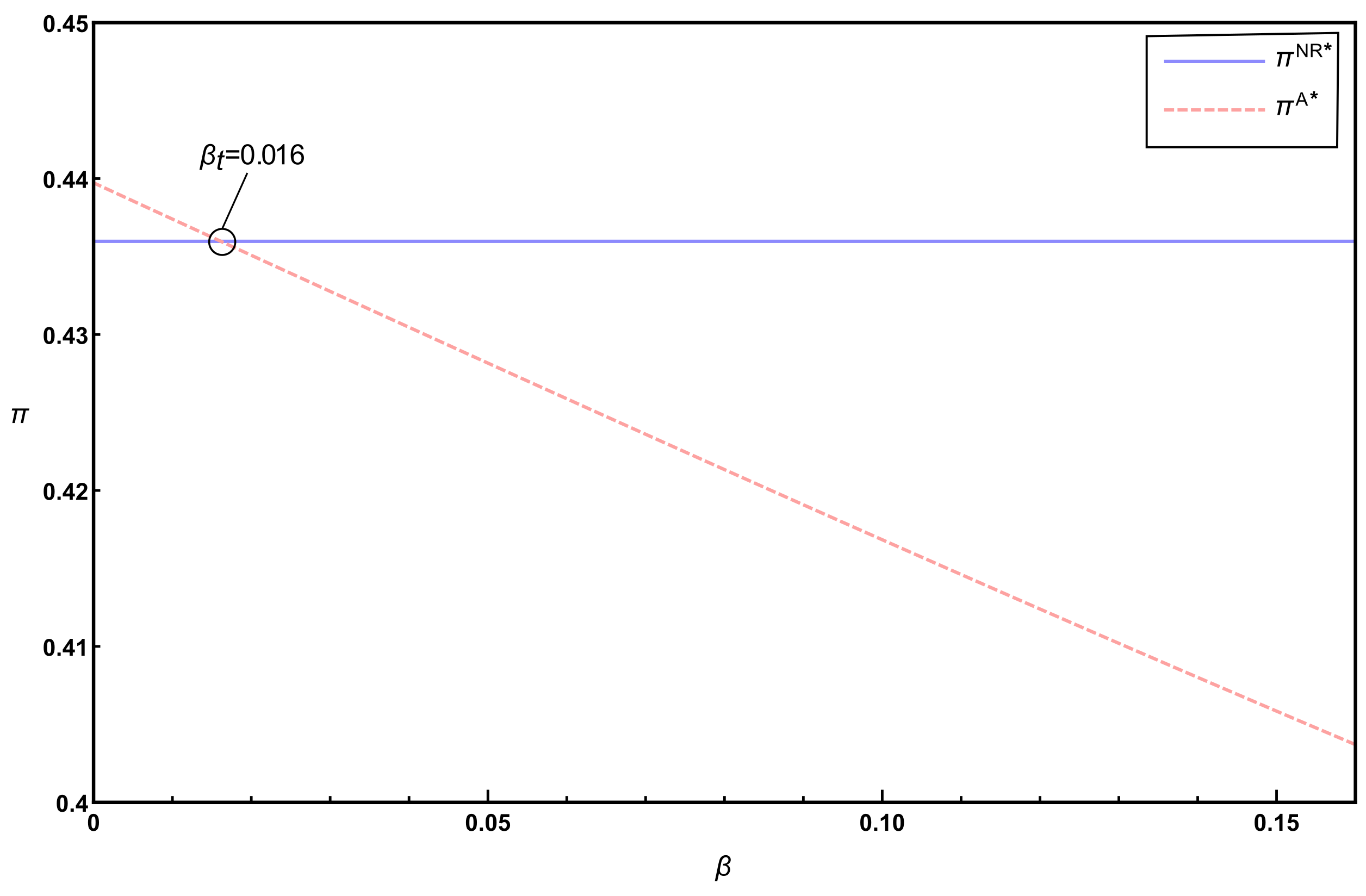
Second, Table 2 indicates that the relationship between and is contingent on the value of . Figure 1 further illustrates such an impact of on the relative magnitude of and . Specifically, when the assimilation effect is low (i.e., below threshold ), the manufacturer should choose to remanufacture. Otherwise, the manufacturer should only produce the new product. This observation implies that the assimilation effect observed from consumers should not be neglected when manufacturers decide whether to undertake remanufacturing activities.
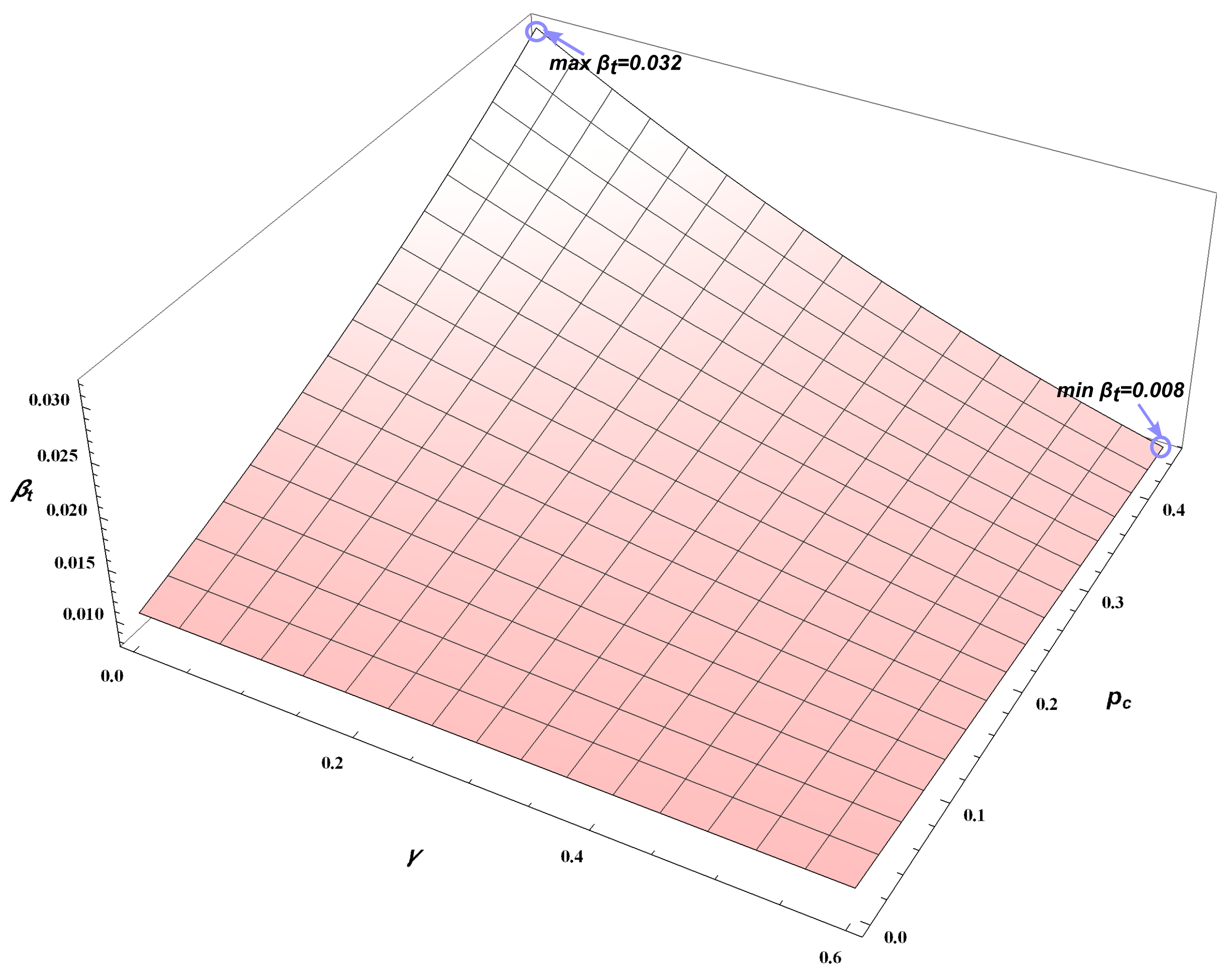
Third, the value of threshold is further affected by both and . Figure 2 illustrates the interactive impact of and on threshold . Particularly, when the carbon emission advantage () is slight, the value of the threshold () increases as carbon trading price () increases. When the carbon emission advantage is large, the value of the threshold decreases as carbon trading price increases.
5.2. Impact of Assimilation Effect
In this section, we examine the impact of the assimilation effect on the optimal outcomes of scenario A. On the basis of empirical evidence reported by Agrawal et al. (2015), which indicated the presence of products remanufactured and sold by the OEM can reduce the perceived value of new products by up to 8%, we assumed that varies between 0 and 0.16.
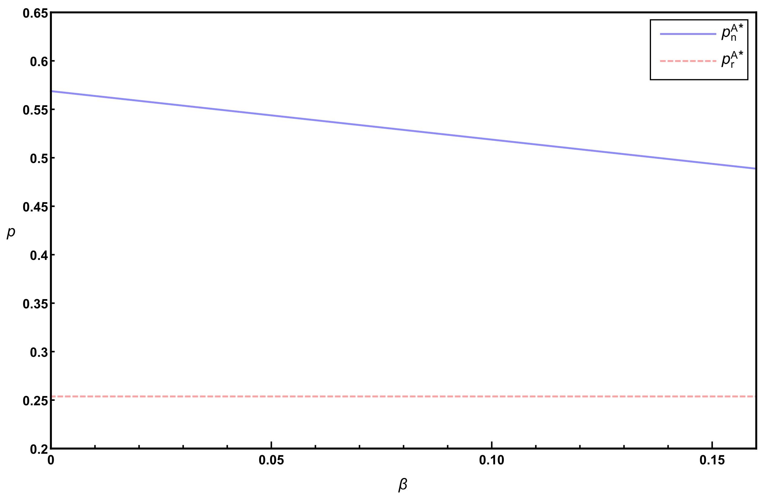
Figure 3 shows that the assimilation effect leads to a negative impact on the retail price of new products. However, it does not impact the retail price of the remanufactured product. In addition, although the retail price of the new product is always higher than that of the remanufactured product, the difference between them narrows down as the assimilation effect increases.
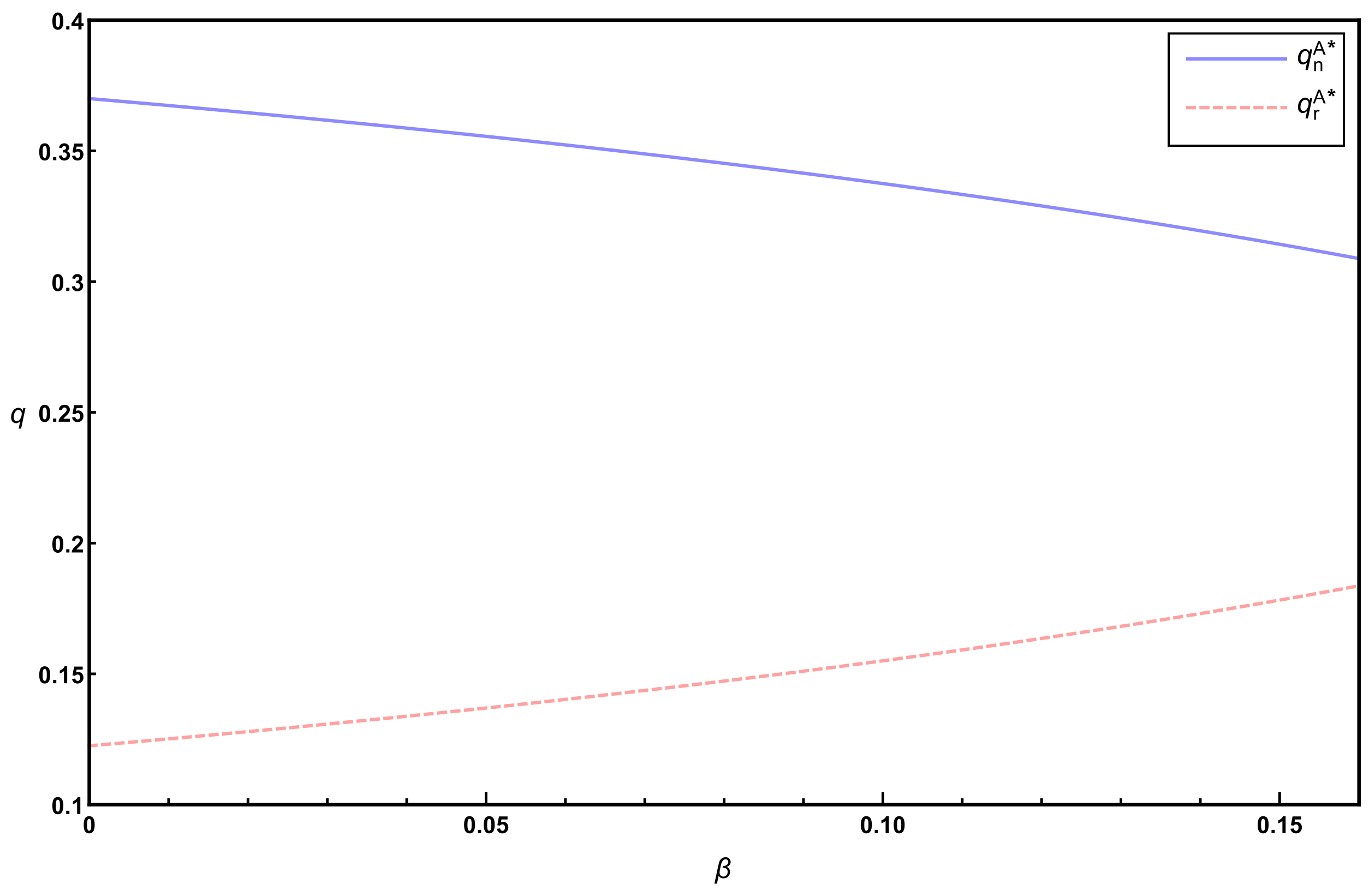
Figure 4 illustrates the impact of the assimilation effect on the sales quantities of new and remanufactured products. As the intensity of the assimilation effect increases, the sales quantity of the new product decreases, while the sales quantity of the remanufactured product increases. The intuition here is that, as the assimilation effect increases, some consumers who originally intended to buy a new product shift to purchasing a remanufactured product.
Figure 3 and Figure 4 show that, as the assimilation effect intensifies, the sales quantity of the remanufactured product increases with its retail price at a constant level, while both the retail price and sales quantity of the new product decrease. This observation suggests that, with the increase in assimilation effect, the manufacturer cannot prevent the decline of new product sales, even if the retail price of the new product is reduced.
5.3. Impact of Carbon Emission Advantage
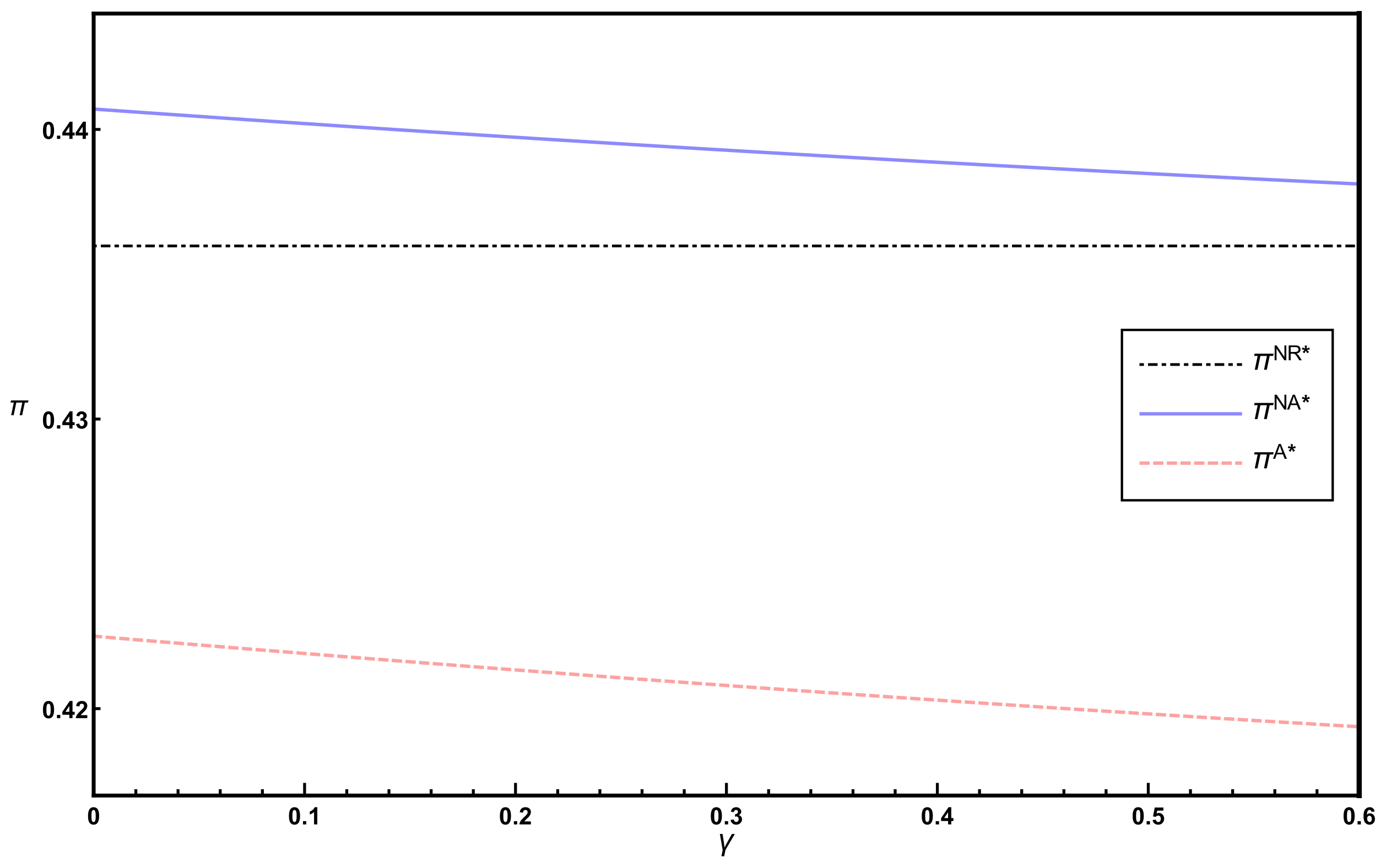
In this subsection, we illustrate the impact of the carbon emission advantage on the equilibrium outcomes of scenarios NR, NA, and A.
Table 3 shows that the retail price of the new product is not affected by , while the remanufactured product’s retail price increases in . In addition, the new product’s price is higher when there is no assimilation effect in the market (i.e., Model NA). Prices of the remanufactured product in Models NA and A are the same. Lastly, Table 3 shows that the sales quantity of the new product increases in , while the sales quantity of the remanufactured product decreases in .
Figure 5 shows that the manufacturer’s profit in scenarios NA and A decreases in . Taking this one step further, with a lower carbon emission advantage (i.e., a higher ), the assimilation effect results in greater loss of profits to the manufacturer. When is sufficiently high, the carbon emission advantage no longer impacts the choice of the manufacturer’s remanufacturing strategy, who always chooses to only produce the new product.
5.4. Impact of Carbon Trading Price
Table 4 summarizes the impact of carbon trading price on the optimal outcomes of scenarios NR,NA, and A. It shows that the retail price of both products in all three scenarios increases with carbon trading price . However, the sales quantity of the new product in the three scenarios decreases as increases.
In addition, Table 4 shows that total carbon emissions in all three scenarios decrease as carbon trading price increases, which implies that the increase in carbon trading price can effectively curb the total carbon emissions of the manufacturer. When the government sets sufficient carbon quotas (i.e., ), profit increases as carbon trading price increases. Therefore, the government should set a reasonable carbon trading price and a reasonable free carbon quota to simultaneously promote environmental protection and economic development.
Table 4 shows that the impact of carbon trading price on the sales quantity of a remanufactured product is not simply one-way. Specifically, when the carbon emission advantage () is low, the quantity of the remanufactured product decreases in . When the carbon emission advantage is high, the quantity of the remanufactured product increases in . Table 4 further illustrates that, when is sufficiently high, the carbon trading price no longer impacts the choice of the manufacturer’s remanufacturing strategy, who always chooses to only produce the new product.
5.5. Consequences of Ignoring Assimilation Effect
In this subsection, we investigate the potential consequences of ignoring the assimilation effect. We compare and , calculating , to assess the level of suboptimality resulting from misinterpretation. We further examine the effects of varying problem parameters on the extent to which the manufacturer’s profits are affected by this misinterpretation.
Table 5 presents the result of the comparison for different levels of , , and . We reached the following conclusions. First, turning a blind eye to the assimilation effect can be very costly to the manufacturer. Table 5 shows that the magnitude of potential loss for the manufacturer reaches up to 56.20% of their profit in some cases. Second, when the degree of the assimilation effect becomes higher, misinterpretation leads to higher losses. Third, the suboptimality gap depends on the competitive position of the remanufactured product. When the carbon emission advantage grows (as decreases), misinterpretation leads to a greater loss. Lastly, when the carbon trading price increases (as increases), misinterpretation leads to a lower loss.
6. Conclusions
In this paper, we explored a monopolistic manufacturer’s choice of remanufacturing engagement strategies under the cap-and-trade regulation of the government. We particularly considered how the assimilation effect affects the manufacturer’s remanufacturing and pricing strategy.
To understand the manufacturer’s choice of remanufacturing engagement strategies, we modeled the manufacturer’s optimal decision making under three different scenarios. Our findings showed that, when the assimilation effect does not exist, the manufacturer should choose to remanufacture. When the assimilation effect exists, the manufacturer’s choice about remanufacturing depends on the intensity of the assimilation effect. In general, the assimilation effect reduce the manufacturer’s incentive to remanufacture. Specifically, there exists a threshold of the assimilation effect. When the assimilation effect is low (i.e., below the threshold), the manufacturer should choose to remanufacture. Otherwise, the manufacturer should only produce the new product.
In addition, our findings show that the value of the threshold of the assimilation effect is further determined by the carbon emission advantage and the carbon trading price. However, when the degree of assimilation effect is significantly higher than the threshold, the carbon trading price and the carbon emission advantage no longer impact the manufacturer’s remanufacturing choice. Our numerical examples suggest that ignoring the assimilation effect can lead to up to 56.2% loss of potential profit for the manufacturer.
6.1. Theoretical Contributions
This research contributes to the literature on remanufacturing strategies and consumer behavior. A growing body of research in operations management focuses on the effect of consumer behavior on the manufacturer’s operational strategies [14,27,28,30,36]. However, there are few previous studies that addressed the issue of manufacturers’ remanufacturing choices under the assimilation effect [2,3]. Motivated by this observation, we report two main findings: (i) the impact of consumers’ assimilation effect on OEM’s pricing and remanufacturing strategies under cap-and-trade regulation, which was not investigated in previous studies; (ii) the potential consequences of ignoring the assimilation effect.
This research also contributes to the cap-and-trade regulation literature in the field of supply chain management. The previous literature largely focused on stationary equilibrium in studying the effect of the cap-and-trade regulation on supply chains’ operational strategies [21,22,24,25]. However, discussion of the remanufacturing strategy considering the assimilation effect is limited. Our research differs from previous studies by exploring the effect of the cap-and-trade regulation on OEMs’ remanufacturing strategies which consider the assimilation effect. The established link between the cap-and-trade regulation research and the enterprises’ remanufacturing strategy under consumer behavior may provide future research avenues.
6.2. Managerial Implications
This research helps in the development of the manufacturing industry by contributing a better understanding of the impact of the assimilation effect. When the assimilation effect exists, an OEM can benefit from remanufacturing engagement via three different mechanisms as follows.
- The OEM can consider adopting more emission reduction technologies, such as green materials, green product design, and green production processes, to improve the carbon emission advantage of the remanufactured products. For example, Apple Inc. is working on improving the disassembly process, such as developing disassembly robotics and artificial intelligence technologies with Carnegie Mellon University, to reduce carbon emissions in remanufacturing.
- The OEM can separately sell new and remanufactured products through different channels to differentiate between them. For example, Apple Inc. only sells remanufactured products on its official website. Similarly, Dyson sells remanufactured products only through specific online channels.
- The OEM can attract more consumers to buy remanufactured products via different mechanisms, such as warranty services, return policy, regret reminder, and consumer education. For example, many manufacturers promise to provide the same warranty policies for their remanufactured products as for new products, such as Apple Inc. and Dyson. Another example is that Dell promises an unconditional 7-day return policy for remanufactured products in China.
This research also presents implications for the government to draft favorable policies for sustainable development. First, the government should set a reasonable carbon trading price and a reasonable free carbon quota to promote environmental protection and economic development at the same time. Second, the government can provide various subsidies to encourage manufacturers to carry out remanufacturing activities. Lastly, the government can give different carbon quotas to manufacturers depending on whether they engage in remanufacturing.
6.3. Limitations
There are several directions worthy of further study. In this paper, we only considered the cap-and-trade regulation. In reality, the government provides various subsidies to encourage manufacturers to carry out remanufacturing activities. With these policies, the manufacturer’s remanufacturing choice may be different from that of this study. In addition, we only considered one type of consumer, namely, those having a lower preference for remanufactured products than for new products. In further research, we can also consider the situation where there are more than one type of consumers. For example, green marketing is increasingly popular to attract green consumers. With green consumers, the remanufactured product may perform differently in the market.
Author Contributions
Conceptualization, T.G. and C.L.; methodology, T.G.; software, T.G.; validation, T.G., C.L. and Y.C.; formal analysis, T.G.; investigation, T.G.; resources, T.G.; data curation, T.G.; writing—original draft preparation, T.G.; writing—review and editing, C.L.; visualization, T.G.; supervision, Y.C.; project administration, Y.C. All authors have read and agreed to the published version of the manuscript.
Funding
This research received no external funding.
Institutional Review Board Statement
Not applicable.
Informed Consent Statement
Not applicable.
Data Availability Statement
Not applicable.
Conflicts of Interest
The authors declare no conflict of interest.
References
- Emissions Cap and Allowances. Website. Available online: https://ec.europa.eu/clima/eu-action/eu-emissions-trading-system-eu-ets/emissions-cap-and-allowances_en (accessed on 27 January 2022).
- Agrawal, V.V.; Atasu, A.; Van Ittersum, K. Remanufacturing, third-party competition, and consumers’ perceived value of new products. Manag. Sci. 2015, 61, 60–72. [Google Scholar] [CrossRef] [Green Version]
- Wu, L.; Liu, L.; Wang, Z. Competitive remanufacturing and pricing strategy with contrast effect and assimilation effect. J. Clean. Prod. 2020, 257, 120333. [Google Scholar] [CrossRef]
- Yang, L.; Hu, Y.; Huang, L. Collecting mode selection in a remanufacturing supply chain under cap-and-trade regulation. Eur. J. Oper. Res. 2020, 287, 480–496. [Google Scholar] [CrossRef]
- Hu, X.; Yang, Z.; Sun, J.; Zhang, Y. Carbon tax or cap-and-trade: Which is more viable for Chinese remanufacturing industry? J. Clean. Prod. 2020, 243, 118606. [Google Scholar] [CrossRef] [Green Version]
- Majumder, P.; Groenevelt, H. Competition in remanufacturing. Prod. Oper. Manag. 2001, 10, 125–141. [Google Scholar] [CrossRef]
- Ferguson, M.E.; Toktay, L.B. The effect of competition on recovery strategies. Prod. Oper. Manag. 2006, 15, 351–368. [Google Scholar] [CrossRef] [Green Version]
- Ferrer, G.; Swaminathan, J.M. Managing New and Remanufactured Products. Manag. Sci. 2006, 52, 15–26. [Google Scholar] [CrossRef] [Green Version]
- Wu, C.H. Price and service competition between new and remanufactured products in a two-echelon supply chain. Int. J. Prod. Econ. 2012, 140, 496–507. [Google Scholar] [CrossRef]
- He, Y. Acquisition pricing and remanufacturing decisions in a closed-loop supply chain. Int. J. Prod. Econ. 2015, 163, 48–60. [Google Scholar] [CrossRef]
- Wu, X.; Zhou, Y. The optimal reverse channel choice under supply chain competition. Eur. J. Oper. Res. 2017, 259, 63–66. [Google Scholar] [CrossRef]
- Wang, N.; He, Q.; Jiang, B. Hybrid closed-loop supply chains with competition in recycling and product markets. Int. J. Prod. Econ. 2019, 217, 246–258. [Google Scholar] [CrossRef]
- Zhang, Z.; Liu, S.; Niu, B. Coordination mechanism of dual-channel closed-loop supply chains considering product quality and return. J. Clean. Prod. 2020, 248, 119273. [Google Scholar] [CrossRef]
- Ma, P.; Gong, Y.; Mirchandani, P. Trade-in for remanufactured products: Pricing with double reference effects. Int. J. Prod. Econ. 2020, 230, 107800. [Google Scholar] [CrossRef]
- Yang, F.; Wang, M.; Ang, S. Optimal remanufacturing decisions in supply chains considering consumers’ anticipated regret and power structures. Transp. Res. Part Logist. Transp. Rev. 2021, 148, 102267. [Google Scholar] [CrossRef]
- Dobos, I. The effects of emission trading on production and inventories in the Arrow–Karlin model. Int. J. Prod. Econ. 2005, 93, 301–308. [Google Scholar] [CrossRef]
- Gong, X.; Zhou, S.X. Optimal production planning with emissions trading. Oper. Res. 2013, 61, 908–924. [Google Scholar] [CrossRef]
- Zakeri, A.; Dehghanian, F.; Fahimnia, B.; Sarkis, J. Carbon pricing versus emissions trading: A supply chain planning perspective. Int. J. Prod. Econ. 2015, 164, 197–205. [Google Scholar] [CrossRef] [Green Version]
- He, P.; Dou, G.; Zhang, W. Optimal production planning and cap setting under cap-and-trade regulation. J. Oper. Res. Soc. 2017, 68, 1094–1105. [Google Scholar] [CrossRef]
- Xu, X.; He, P.; Xu, H.; Zhang, Q. Supply chain coordination with green technology under cap-and-trade regulation. Int. J. Prod. Econ. 2017, 183, 433–442. [Google Scholar] [CrossRef]
- Taleizadeh, A.A.; Shahriari, M.; Sana, S.S. Pricing and Coordination Strategies in a Dual Channel Supply Chain with Green Production under Cap and Trade Regulation. Sustainability 2021, 13, 12232. [Google Scholar] [CrossRef]
- Bai, Q.; Xu, J.; Zhang, Y. Emission reduction decision and coordination of a make-to-order supply chain with two products under cap-and-trade regulation. Comput. Ind. Eng. 2018, 119, 131–145. [Google Scholar] [CrossRef]
- Wang, M.; Zhao, L.; Herty, M. Joint replenishment and carbon trading in fresh food supply chains. Eur. J. Oper. Res. 2019, 277, 561–573. [Google Scholar] [CrossRef]
- Zhang, G.; Zhang, X.; Sun, H.; Zhao, X. Three-echelon closed-loop supply chain network equilibrium under cap-and-trade regulation. Sustainability 2021, 13, 6472. [Google Scholar] [CrossRef]
- Zhao, F.; Liu, F.; Hao, H.; Liu, Z. Carbon emission reduction strategy for energy users in China. Sustainability 2020, 12, 6498. [Google Scholar] [CrossRef]
- Donohue, K.; Özer, Ö.; Zheng, Y. Behavioral Operations: Past, Present, and Future. Manuf. Serv. Oper. Manag. 2020, 22, 191–202. [Google Scholar] [CrossRef] [Green Version]
- Li, K.J.; Jain, S. Behavior-Based Pricing: An Analysis of the Impact of Peer-Induced Fairness. Manag. Sci. 2016, 62, 2705–2721. [Google Scholar] [CrossRef]
- He, Y.; Xu, Q.; Xu, B.; Wu, P. Supply chain coordination in quality improvement with reference effects. J. Oper. Res. Soc. 2016, 67, 1158–1168. [Google Scholar] [CrossRef]
- Ma, Z.J.; Zhou, Q.; Dai, Y.; Guan, G.F. To license or not to license remanufacturing business? Sustainability 2018, 10, 347. [Google Scholar] [CrossRef] [Green Version]
- Zou, Z.; Wang, F.; Lai, X.; Hong, J. How does licensing remanufacturing affect the supply chain considering customer environmental awareness? Sustainability 2019, 11, 1898. [Google Scholar] [CrossRef] [Green Version]
- Jia, D.; Li, S. Optimal decisions and distribution channel choice of closed-loop supply chain when e-retailer offers online marketplace. J. Clean. Prod. 2020, 265, 121767. [Google Scholar] [CrossRef]
- Huang, H.; Meng, Q.; Xu, H.; Zhou, Y. Cost information sharing under competition in remanufacturing. Int. J. Prod. Res. 2019, 57, 6579–6592. [Google Scholar] [CrossRef]
- Subramanian, R.; Ferguson, M.E.; Beril Toktay, L. Remanufacturing and the component commonality decision. Prod. Oper. Manag. 2013, 22, 36–53. [Google Scholar] [CrossRef]
- Wu, X.; Zhou, Y. Buyer-specific versus uniform pricing in a closed-loop supply chain with third-party remanufacturing. Eur. J. Oper. Res. 2019, 273, 548–560. [Google Scholar] [CrossRef]
- Abbey, J.D.; Kleber, R.; Souza, G.C.; Voigt, G. The role of perceived quality risk in pricing remanufactured products. Prod. Oper. Manag. 2017, 26, 100–115. [Google Scholar] [CrossRef]
- Duan, C.; Xiu, G.; Yao, F. Multi-period e-closed-loop supply chain network considering consumers’ preference for products and ai-push. Sustainability 2019, 11, 4571. [Google Scholar] [CrossRef] [Green Version]
Figure 1.
Comparison of manufacturer profits under Models NR and A with different assimilation effect intensities (, and ).
Figure 1.
Comparison of manufacturer profits under Models NR and A with different assimilation effect intensities (, and ).

Figure 2.
Interactive impact of and on threshold value (, , , and ).

Figure 3.
Impact of parameter on retail prices (, , , , , and ).

Figure 4.
Impact of parameter on sales quantity (, , , , , and ).

Figure 5.
Impact of parameter on profits (, , , , , and ).


Table 1.
Values of problem parameters.
| Parameters | Values |
|---|---|
| 0.50 | |
| 0.08 | |
| 0.20 | |
| 0.25 | |
| 0.15 | |
| 0.10 | |
| 1.00 |
Table 2.
Comparison of impact of , , and on manufacturer profit under Models NR, NA, and A. Results based on all instances with , and .
Table 2.
Comparison of impact of , , and on manufacturer profit under Models NR, NA, and A. Results based on all instances with , and .
| 0.2 | 0.05 | 0.2491 | 0.2519 | 0.2494 | 0.2491 | 0.2519 | 0.2329 | 0.2491 | 0.2519 | 0.2145 |
| 0.25 | 0.4360 | 0.4397 | 0.4374 | 0.4360 | 0.4397 | 0.4213 | 0.4360 | 0.4397 | 0.4037 | |
| 0.45 | 0.6233 | 0.6282 | 0.6259 | 0.6233 | 0.6282 | 0.6105 | 0.6233 | 0.6282 | 0.5938 | |
| 0.4 | 0.05 | 0.2491 | 0.2517 | 0.2493 | 0.2491 | 0.2517 | 0.2328 | 0.2491 | 0.2517 | 0.2143 |
| 0.25 | 0.4360 | 0.4389 | 0.4365 | 0.4360 | 0.4389 | 0.4203 | 0.4360 | 0.4389 | 0.4024 | |
| 0.45 | 0.6233 | 0.6265 | 0.6242 | 0.6233 | 0.6265 | 0.6084 | 0.6233 | 0.6265 | 0.5911 | |
| 0.6 | 0.05 | 0.2491 | 0.2516 | 0.2492 | 0.2491 | 0.2516 | 0.2326 | 0.2491 | 0.2516 | 0.2141 |
| 0.25 | 0.4360 | 0.4381 | 0.4357 | 0.4360 | 0.4381 | 0.4194 | 0.4360 | 0.4381 | 0.4012 | |
| 0.45 | 0.6233 | 0.6251 | 0.6228 | 0.6233 | 0.6251 | 0.6067 | 0.6233 | 0.6251 | 0.5889 | |
Table 3.
Comparison of impact of on manufacturer’s optimal outcomes under Models NR, NA, and A. Results based on all instances with .
Table 3.
Comparison of impact of on manufacturer’s optimal outcomes under Models NR, NA, and A. Results based on all instances with .
| Model NR | Model NA | Model A | ||||||||||||||
| 0.1 | 0.569 | 0.431 | 0.065 | 0.4360 | 0.569 | 0.252 | 0.366 | 0.130 | 0.057 | 0.4402 | 0.529 | 0.252 | 0.340 | 0.155 | 0.053 | 0.4219 |
| 0.2 | 0.569 | 0.431 | 0.065 | 0.4360 | 0.569 | 0.254 | 0.370 | 0.123 | 0.059 | 0.4397 | 0.529 | 0.254 | 0.345 | 0.147 | 0.056 | 0.4213 |
| 0.3 | 0.569 | 0.431 | 0.065 | 0.4360 | 0.569 | 0.256 | 0.374 | 0.115 | 0.061 | 0.4392 | 0.529 | 0.256 | 0.350 | 0.139 | 0.059 | 0.4208 |
| 0.4 | 0.569 | 0.431 | 0.065 | 0.4360 | 0.569 | 0.258 | 0.378 | 0.108 | 0.063 | 0.4389 | 0.529 | 0.258 | 0.354 | 0.131 | 0.061 | 0.4203 |
| 0.5 | 0.569 | 0.431 | 0.065 | 0.4360 | 0.569 | 0.259 | 0.381 | 0.100 | 0.065 | 0.4384 | 0.529 | 0.259 | 0.359 | 0.123 | 0.063 | 0.4198 |
| 0.6 | 0.569 | 0.431 | 0.065 | 0.4360 | 0.569 | 0.261 | 0.385 | 0.093 | 0.066 | 0.4381 | 0.529 | 0.261 | 0.363 | 0.114 | 0.065 | 0.4194 |
Table 4.
Comparison of manufacturer’s optimal outcomes under Models NR, NA, and A. Results based on all instances with .
Table 4.
Comparison of manufacturer’s optimal outcomes under Models NR, NA, and A. Results based on all instances with .
| Model NR | Model NA | Model A | |||||||||||||||
|---|---|---|---|---|---|---|---|---|---|---|---|---|---|---|---|---|---|
| 0.2 | 0.05 | 0.554 | 0.446 | 0.067 | 0.249 | 0.554 | 0.250 | 0.394 | 0.105 | 0.062 | 0.252 | 0.514 | 0.251 | 0.374 | 0.125 | 0.060 | 0.233 |
| 0.25 | 0.569 | 0.431 | 0.065 | 0.436 | 0.569 | 0.254 | 0.370 | 0.123 | 0.059 | 0.440 | 0.529 | 0.254 | 0.345 | 0.147 | 0.056 | 0.421 | |
| 0.45 | 0.584 | 0.416 | 0.062 | 0.623 | 0.584 | 0.257 | 0.346 | 0.141 | 0.056 | 0.628 | 0.544 | 0.257 | 0.317 | 0.170 | 0.053 | 0.611 | |
| 0.4 | 0.05 | 0.554 | 0.446 | 0.067 | 0.249 | 0.554 | 0.252 | 0.396 | 0.102 | 0.065 | 0.252 | 0.514 | 0.252 | 0.376 | 0.121 | 0.064 | 0.233 |
| 0.25 | 0.569 | 0.431 | 0.065 | 0.436 | 0.569 | 0.258 | 0.378 | 0.108 | 0.063 | 0.439 | 0.529 | 0.258 | 0.354 | 0.131 | 0.061 | 0.420 | |
| 0.45 | 0.584 | 0.416 | 0.062 | 0.623 | 0.584 | 0.264 | 0.360 | 0.114 | 0.061 | 0.627 | 0.544 | 0.264 | 0.333 | 0.140 | 0.058 | 0.608 | |
| 0.6 | 0.05 | 0.554 | 0.446 | 0.067 | 0.249 | 0.554 | 0.252 | 0.397 | 0.099 | 0.068 | 0.252 | 0.514 | 0.253 | 0.377 | 0.118 | 0.067 | 0.233 |
| 0.25 | 0.569 | 0.431 | 0.065 | 0.436 | 0.569 | 0.261 | 0.385 | 0.093 | 0.066 | 0.438 | 0.529 | 0.261 | 0.363 | 0.114 | 0.065 | 0.419 | |
| 0.45 | 0.584 | 0.416 | 0.062 | 0.623 | 0.584 | 0.270 | 0.373 | 0.087 | 0.064 | 0.625 | 0.544 | 0.270 | 0.349 | 0.111 | 0.062 | 0.607 | |
Table 5.
OEM percentage suboptimality gap resulting when assimilation effect is ignored. Results based on all instances with .
Table 5.
OEM percentage suboptimality gap resulting when assimilation effect is ignored. Results based on all instances with .
| 0.02 | 0.04 | 0.08 | 0.12 | 0.16 | ||
|---|---|---|---|---|---|---|
| 0.05 | 3.73% | 8.12% | 19.31% | 34.76% | 56.20% | |
| 0.15 | 2.86% | 6.17% | 14.49% | 25.71% | 40.94% | |
| 0.25 | 2.35% | 5.09% | 11.83% | 20.81% | 32.84% | |
| 0.35 | 2.05% | 4.39% | 10.16% | 17.75% | 27.84% | |
| 0.45 | 1.83% | 3.91% | 9.00% | 15.67% | 24.46% | |
| 0.05 | 3.72% | 8.09% | 19.25% | 34.65% | 56.04% | |
| 0.15 | 2.82% | 6.10% | 14.34% | 25.46% | 40.57% | |
| 0.25 | 2.32% | 4.99% | 11.63% | 20.47% | 32.34% | |
| 0.35 | 1.99% | 4.28% | 9.91% | 17.34% | 27.24% | |
| 0.45 | 1.77% | 3.79% | 8.73% | 15.21% | 23.78% | |
| 0.05 | 3.70% | 8.06% | 19.18% | 34.55% | 55.89% | |
| 0.15 | 2.79% | 6.04% | 14.19% | 25.20% | 40.20% | |
| 0.25 | 2.27% | 4.90% | 11.42% | 20.12% | 31.83% | |
| 0.35 | 1.94% | 4.17% | 9.66% | 16.93% | 26.63% | |
| 0.45 | 1.71% | 3.66% | 8.45% | 14.75% | 23.10% | |
Publisher’s Note: MDPI stays neutral with regard to jurisdictional claims in published maps and institutional affiliations. |
© 2022 by the authors. Licensee MDPI, Basel, Switzerland. This article is an open access article distributed under the terms and conditions of the Creative Commons Attribution (CC BY) license (https://creativecommons.org/licenses/by/4.0/).
Share and Cite
MDPI and ACS Style
Guo, T.; Li, C.; Chen, Y. Remanufacturing Strategy under Cap-and-Trade Regulation in the Presence of Assimilation Effect. Sustainability 2022, 14, 2878. https://doi.org/10.3390/su14052878
AMA Style
Guo T, Li C, Chen Y. Remanufacturing Strategy under Cap-and-Trade Regulation in the Presence of Assimilation Effect. Sustainability. 2022; 14(5):2878. https://doi.org/10.3390/su14052878
Chicago/Turabian StyleGuo, Tianyi, Chaonan Li, and Yan Chen. 2022. "Remanufacturing Strategy under Cap-and-Trade Regulation in the Presence of Assimilation Effect" Sustainability 14, no. 5: 2878. https://doi.org/10.3390/su14052878
Note that from the first issue of 2016, this journal uses article numbers instead of page numbers. See further details here.