
Surface Ozone Pollution: Trends, Meteorological Influences, and Chemical Precursors in Portugal


1
LEPABE—Laboratory for Process Engineering, Environment, Biotechnology and Energy, Faculty of Engineering, University of Porto, Rua Dr. Roberto Frias, 4200-465 Porto, Portugal
2
AliCE—Associate Laboratory in Chemical Engineering, Faculty of Engineering, University of Porto, Rua Dr. Roberto Frias, 4200-465 Porto, Portugal
*
Author to whom correspondence should be addressed.
Sustainability 2022, 14(4), 2383; https://doi.org/10.3390/su14042383
Submission received: 22 December 2021
/
Revised: 8 February 2022
/
Accepted: 17 February 2022
/
Published: 19 February 2022
(This article belongs to the Special Issue Air Quality Characterisation and Modelling)
Abstract
:Surface ozone (O3) is a secondary air pollutant, harmful to human health and vegetation. To provide a long-term study of O3 concentrations in Portugal (study period: 2009–2019), a statistical analysis of ozone trends in rural stations (where the highest concentrations can be found) was first performed. Additionally, the effect of nitrogen oxides (NOx) and meteorological variables on O3 concentrations were evaluated in different environments in northern Portugal. A decreasing trend of O3 concentrations was observed in almost all monitoring stations. However, several exceedances to the standard values legislated for human health and vegetation protection were recorded. Daily and seasonal O3 profiles showed high concentrations in the afternoon and summer (for all inland rural stations) or spring (for Portuguese islands). The high number of groups obtained from the cluster analysis showed the difference of ozone behaviour amongst the existent rural stations, highlighting the effectiveness of the current geographical distribution of monitoring stations. Stronger correlations between O3, NO, and NO2 were detected at the urban site, indicating that the O3 concentration was more NOx-sensitive in urban environments. Solar radiation showed a higher correlation with O3 concentration regarding the meteorological influence. The wind and pollutants transport must also be considered in air quality studies. The presented results enable the definition of air quality policies to prevent and/or mitigate unfavourable outcomes from O3 pollution.
1. Introduction
With the constant increase of air pollutants emissions since the Industrial Revolution, an increase of ozone (O3) near the Earth’s surface has been observed [1,2,3]. This pollutant is a powerful oxidant, affecting human health by causing respiratory and cardiovascular diseases [4]. It also affects vegetation and ecosystems, leading to crop yield and biodiversity losses [5,6]. A total value of 769.2 billion USD loss equivalent to decreases in agricultural production and the occurrence of respiratory diseases and mortality could be ascribed to O3 exposure in China [7].
O3 is a secondary pollutant resultant of the reaction between nitrogen oxides (NOx) and volatile organic compounds (VOCs) released to the atmosphere from natural and (mostly) anthropogenic activities [1]. The photochemical regime for surface ozone production determines the sensitivity of O3 to anthropogenic sources. Usually, urban and suburban zones are VOC-limited due to higher levels of NOx emissions, while less-populated zones (rural sites) are NOx-limited [8,9]. Domínguez-López et al. [10] analysed the effect of NOx (NO2 and NO) concentrations in surface ozone at different locations through a spatial and temporal variation study. An opposite daily variance was observed between O3, NO, and NO2 concentrations in urban and suburban areas. Maximum ozone concentrations were observed in the early afternoon, while NOx concentrations usually achieve two peaks (early morning and late afternoon). In rural sites, no hourly peak O3 or NOx was observed. Sun et al. [11] showed that rural sites presented O3 levels (approximately) 30 μg m−3 higher than urban regions in the study period of 1990–2019. Therefore, rural and remote areas are the object of many studies, as the highest ozone levels are found there [12,13]. Several factors (such as higher average temperatures and usually lower NOx emissions) lead to a more significant accumulation of this pollutant in these areas. There is also evidence of the influence of other chemical air pollutants in O3 tropospheric levels, such as anthropogenic aerosols, that can affect O3 photolysis rates directly (through earth radiation scattering) and indirectly (due to the formation of clouds), leading to a weaker surface insolation [14,15]. Li et al. [9] found that the increase of O3 concentrations (predicted due to the decrease in NOx emissions) was in fact generated by the abrupt decrease in PM2.5, resulting in a reduction of aerosols as a sink of HO2, stimulating the production of this secondary pollutant. O3 is known for its complex formation, depending on many variables. In addition to chemical precursors, meteorological variables are also considered in studying and predicting ozone levels. In different parts of the globe, Fang et al. [16] and Afonso and Pires [17] reached the same results through correlation analysis: ozone shows a positive correlation with temperature, meaning it increases with the increase of this meteorological parameter, and the opposite with relative humidity, that shows a negative correlation with O3. Other variables that can lead to the formation or elimination of surface O3 are air pressure, wind speed, and direction. The same authors also concluded that O3 has a negative correlation with local air pressure and a positive correlation with wind speed. Being a pollutant resultant of a radiation-induced chemical reaction, O3 shows higher levels with clear skies, which is also related to the presence of anticyclones. The association of O3 concentrations with different weather conditions is more detailed in Domínguez-López et al. [10].
In Portugal, surface O3 pollution has been characterised in many studies [17,18,19,20,21], especially in the northern [17,22,23,24] and rural regions [13,25,26]. To complete the study area with more recent data and improve O3 trends’ understanding in Portugal, this study aims to (i) determine the evolution of O3 levels in Portuguese rural stations, focusing on exceedances to legally imposed levels for human and vegetation protection; (ii) compare the relationship between the O3 concentrations and one of its precursors (NOx) for different environments; and (iii) evaluate the effect of meteorological conditions in ozone concentrations. This study presents a long-term characterisation (data from more than 10 years) of O3 concentrations from different environments, including regions in which no similar study was performed yet. In addition, the statistical models were applied to explanatory variables that were selected based on the knowledge of the chemical reactions of O3 production. This integration enables better performance in predicting O3 concentrations, allowing, in advance, to prevent and/or mitigate possible unfavourable outcomes.
2. Materials and Methods
2.1. Ozone Concentration Analysis at Rural Stations
For a better understanding of the trends and levels of surface ozone at rural sites, the study period 2009 to 2019 was selected. Table 1 represents the geographical information of the 15 existing rural stations [27]. The minimum distance to the seashore was estimated using a tool available on Google Earth that allows measuring the distance between two points. Figure S1 presents the map with the geographical distribution of the rural sites.
The statistical analyses were performed only for O3 concentrations recorded at stations with a monitoring efficiency higher than 75%. The temporal trend of O3 concentrations was assessed by determining the annual average concentration for each station. The exceedances to all thresholds presented in the current legislation were determined: (i) alert (240 μm m−3) and information (180 μm m−3) threshold, (ii) target value for human protection (120 μm m−3), and (iii) AOT40, representative of vegetation protection, as a target value (8000 μg m−3 h) and a long-term goal (6000 μg m−3 h) [28]. The data collected at four rural sites from different regions in Portugal were then used to characterise the spatial variability of O3 concentrations. Histograms with density functions and violin plots were plotted in Python.
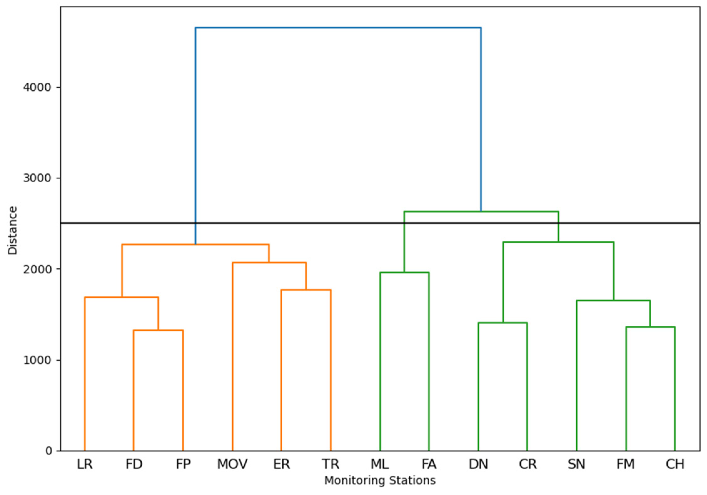
Cluster analysis (CA) was applied to the rural stations to evaluate the representativeness of the stations with local O3 measurement. This analysis aims to group monitoring sites in the same class/cluster according to the observed behaviour (daily concentration fluctuation) of collected O3 data. A hierarchical clustering method was used, generating solutions with 1 to n clusters. Ward’s minimum variance method was used to determine the cluster distance. A dendrogram (or tree diagram—graphical representation of hierarchical CA) was determined for each year. Based on the obtained dendrograms, a matrix of relative frequencies was used to pair each monitoring site in clusters, using measured O3 concentrations. This matrix enables the definition of the number of different O3 behaviours in the studied remote areas. Daily profiles of O3 concentrations were determined for each group of monitoring sites and the daily distribution of the daily maximum values using Microsoft Excel Macros developed by the authors.
2.2. O3 and NOx Relationship
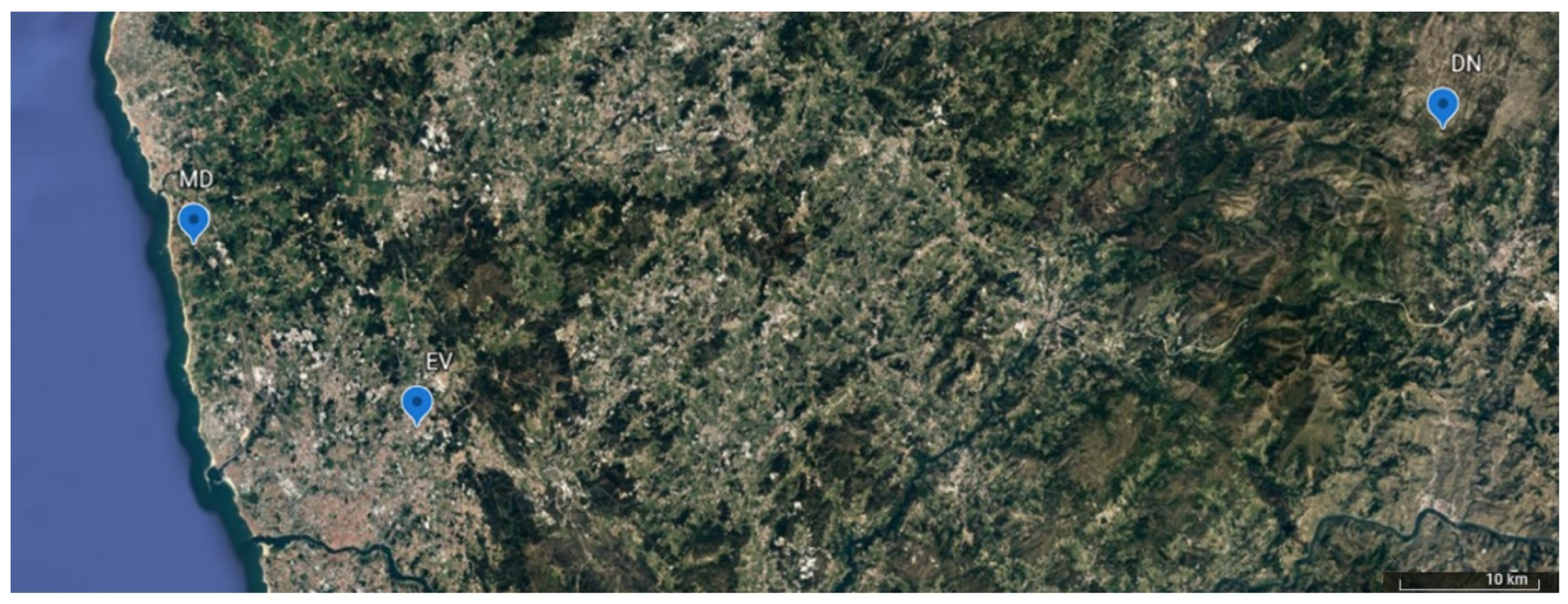
For an evaluation of the relationship between O3 and its chemical precursor (nitrogen oxides, NO, and NO2), urban (Ermesinde-Valongo, EV), suburban (Mindelo-Vila do Conde, MD), and rural (Douro Norte, DN) stations were selected (see Figure 1). Considering data availability (O3 and its chemical precursors monitoring efficiency close or higher than 75% for the selected monitoring stations), the studied period was 2019. A correlation matrix (Pearson’s Correlation—PC) was obtained with a O3, NO2, NO, and NO2/NO ratio for each monitoring station. Multiple linear regression (MLR) was applied to better understand the NOx influence in O3 production. The method aims to develop a linear model to predict the output variable (Y) with several predictor ones (Xi), having each one a regression coefficient (bi, i = 1, n) with b0 being the Y-intercept, as shown in Equation (1).
Y = b0 + ∑biXi
The statistical significance of correlation coefficients and MLR parameters was evaluated by applying a t-test with a significance level of 5%.
2.3. Meteorological Data and O3 Relationship
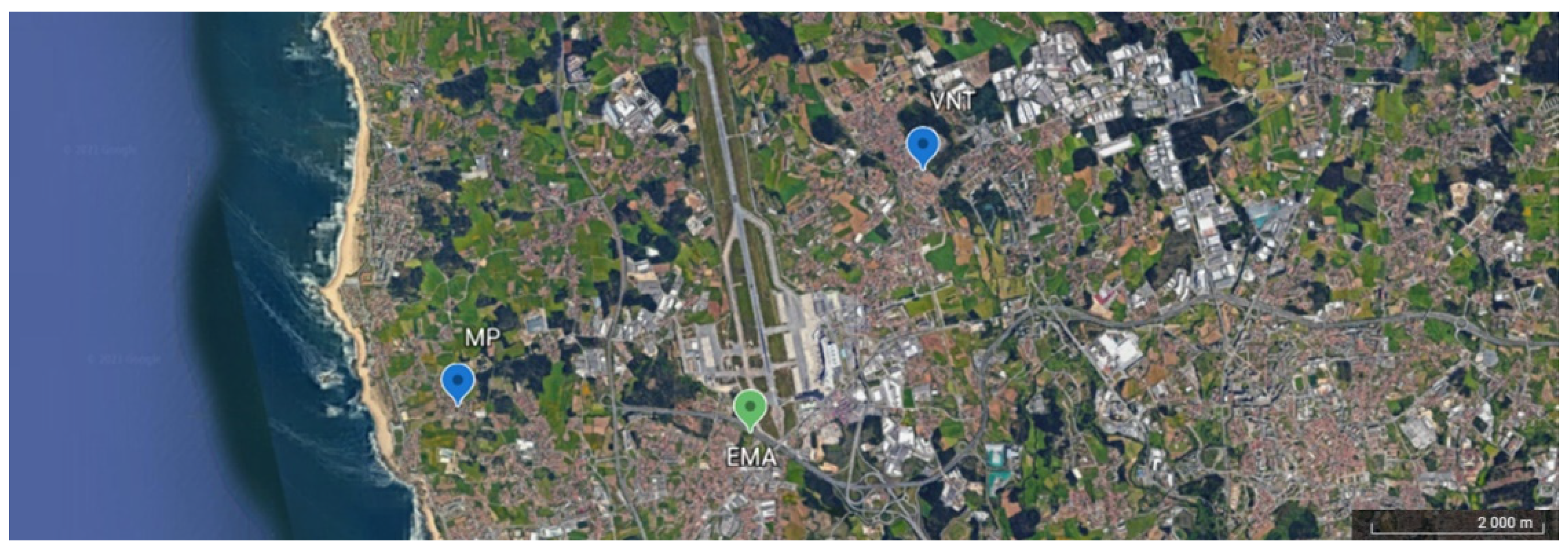
A similar analysis was performed to assess the effect of meteorological conditions on O3 concentrations using data collected at Pedras Rubras/Aeródromo EMA (Automatic Meteorological Station) and the O3 of Meco-Perafita (MP) and VNTelha-Maia (VNT), which are both suburban stations (Figure 2). The data evaluated corresponds to 2015 (the year in which selected monitoring stations presented a monitoring efficiency close to or higher than 75%). The meteorological data evaluated are mean air pressure (P, in hPa), mean air temperature (T, in °C), relative humidity (RH, in %), wind direction (WD, in degrees), wind speed (WS, in m/s), and solar radiation (SR, in kJ/m2). The data was provided by the national meteorological, seismic, and oceanographic organisation IPMA (Instituto Português do Mar e da Atmosfera, website: https://www.ipma.pt/en/index.html, accessed on 15 March 2021).
The PC and MLR methods were applied to the meteorological parameters (except for wind data) and O3 concentrations for annual quarters. A wind rose was developed to visualise the wind speed and direction registered, resorting to a MATLAB-coded program. To evaluate the wind speed and direction influence on ozone, violin plots were used to represent the frequency of O3 concentration in each wind direction and speed interval considered.
3. Results and Discussion
3.1. Surface Ozone at Rural Stations
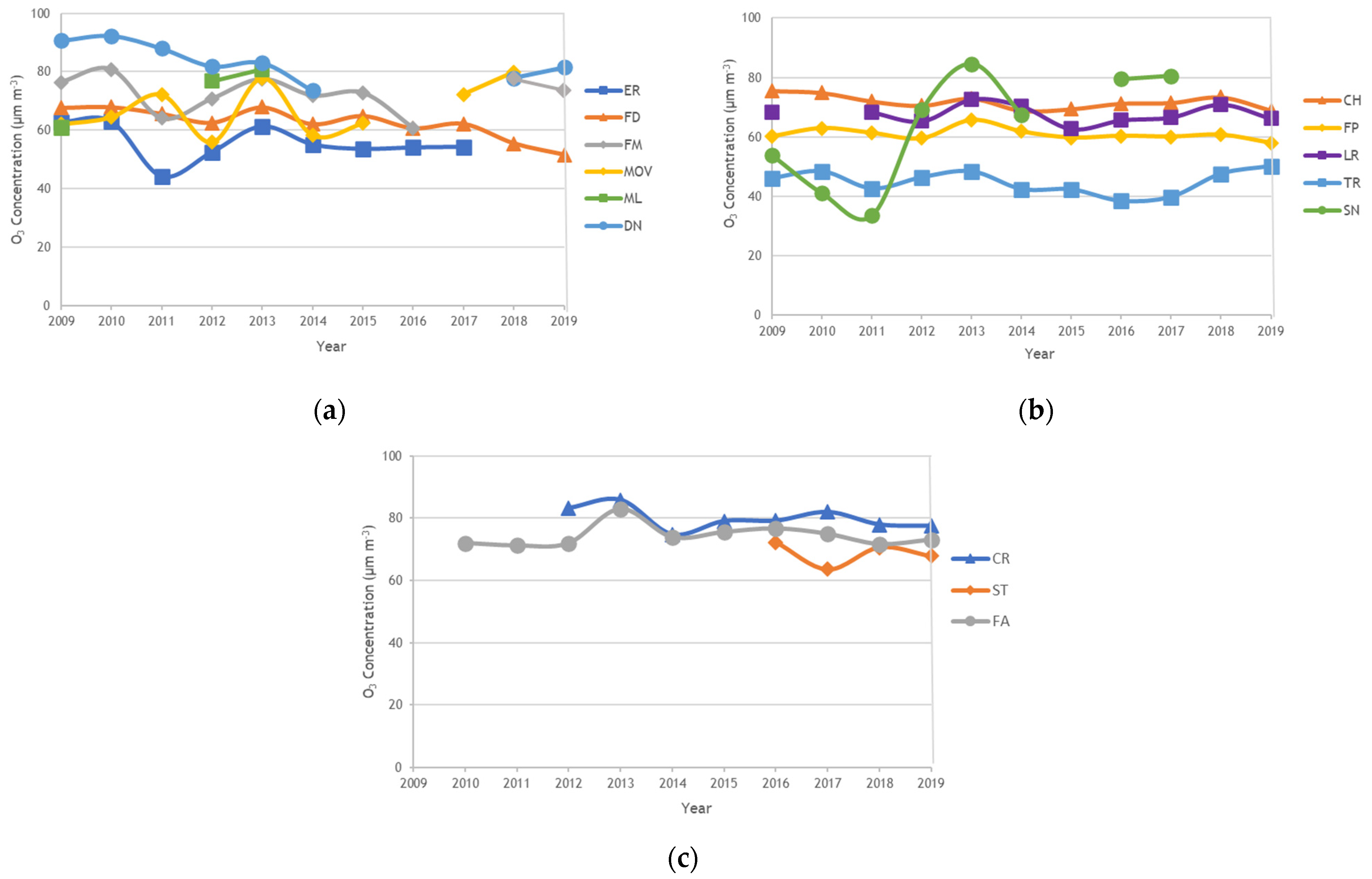
Table 2 presents the monitoring efficiency of each station during the study period. Figure 3 shows the annual average O3 concentrations at each monitoring station in the studied period. The highest annual average O3 concentrations were achieved at the DN, CR, SN, FA, FM, and ML sites. The highest values were observed for almost all stations during the period of 2001–2008 [13], except for the SN station, which shows a significant variance in mean values during the study period (Figure 3b). O3 concentrations have been decreasing at most stations with rates between −0.12 and −1.35 μg m−3 year−1. This behaviour has already been reported at rural Portuguese sites by Pires et al. [13] between 2001 and 2008. The exceptions to this trend are stations ML and SN, with high increase rates of 5.04 and 5.06 μg m−3 year−1, respectively, and those with lower increase rates, the MOV (1.26 μg m−3 year−1) and FA (0.06 μg m−3 year−1) stations. Another study reported similar results for the MOV, FM, and ER stations between 2009 and 2011 [29]. Borrego et al. [22] detected a slight but significant decrease in ozone levels since 2006 in Portuguese rural stations. Yan et al. [30] reported decreases in rural European monitoring stations between 1995 and 2014. In the shorter period of 2000 to 2014, the decrease of O3 concentrations was also registered by Chang et al. [31] and Proietti et al. [32] in Europe. The latter study reported a more significant decrease rate (−0.22 μg m−3 year−1) in Mediterranean Europe.
Table 3 shows the exceedances to EU standard values for human protection (alert threshold, information threshold, and target value) during the study period. The alert threshold (240 μg m−3) was exceeded in the DN, FM, and MOV stations. Apart from the TR, CR, ST, and FA stations, the information threshold (180 μg m−3) was exceeded in all others. The highest number of exceedances was determined for the DN station. It is also the station with the highest number of exceedances in the period under study, followed by the FM station. The highest number of exceedances for both standard limits was determined in 2010. Regarding the target value for human health protection (120 μg m−3), DN, CH, and FM were the three stations that recorded the most exceedances (in the respective order). In the Portuguese islands, exceedances to this limit were also observed. However, in ER, LR, SN, CR, TR, ST, and FA stations, exceedances were below 25 on average over 3 years, meaning that their O3 concentrations were within the legislation requirements. However, none of the stations complied with the long-term objective imposed for human health protection.
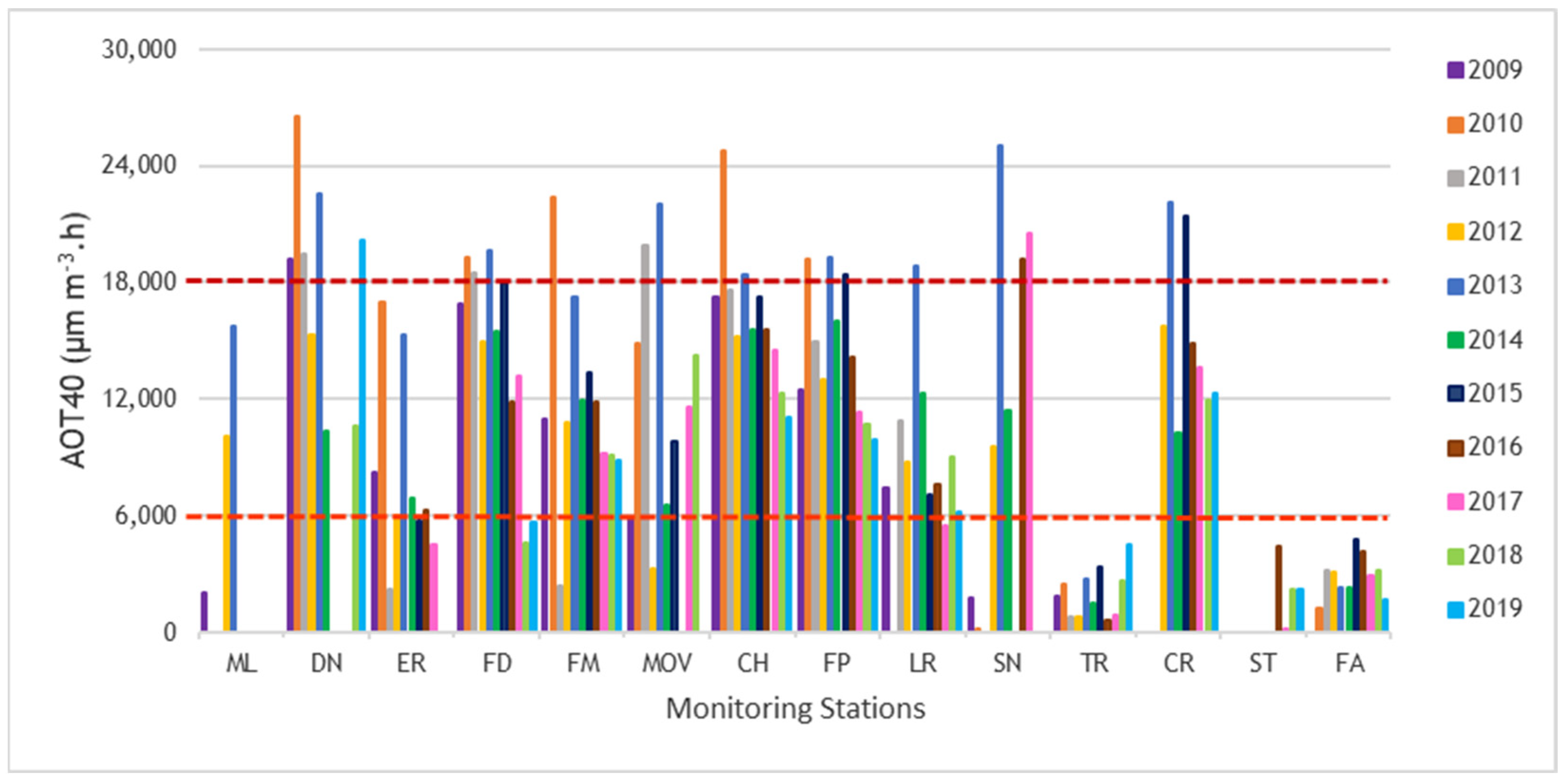
The EU legislation presents two different values (AOT40) for the long-term goal and the target value for short-term exposition impact estimations for vegetation protection. Figure 4 presents the calculated AOT40 values at each monitoring site, showing the exceedances to these two parameters. Both legislated values were not surpassed at the TR, ST, and FA stations (the last two are in the Portuguese islands).
Four stations were selected to deeply analyse the O3 behaviour in different regions of Portugal (representing North, Centre, and South Regions and Islands). A histogram with frequency distribution for 2012 and violin plots representing monthly ozone concentrations are displayed for each selected station in Figure S3. The station located at a higher altitude (DN) presented the highest concentration levels, with more elevated minimum levels. The inner located station (FD) showed significant variation in the ozone concentration, with a maximum value not going far beyond 150 μg m−3 unlike DN, whose peak reached 250 μg m−3. The other inland station, located further south (FP), showed similar behaviour to the FD station but reached a higher peak ozone level. All inland stations show peak values in summer, but higher mean concentrations in spring. This characteristic is known in northern hemisphere remote locations, where the peak concentrations can be related to a higher stratosphere-troposphere exchange or be enhanced by increased solar radiation after winter months with accumulated NOx and VOC levels [33,34]. In the station at sea level (FA), the lowest ozone concentrations (not surpassing 120 μg m−3) were observed. In all the mentioned stations, the maximum daily concentration occurs at 15 h–16 h, except for the FA station, which shows an almost non-existing daily variation of the concentration. A study conducted in southern Spain also presented that the higher O3 values appear in high-altitude locations, usually closer to the sea [35]. DN station was the focus of other studies due to register the majority of Portuguese legislated threshold exceedances. Carvalho et al. [25] attribute DN’s high levels to long-range transport of pollutants from NE winds, and Borrego et al. [22] showed that background values contribute more than 50% to the local O3 concentrations.
CA was performed to group monitoring stations according to O3 data for each year. Figure 5 shows, as an example, the dendrogram obtained with data from 2012, forming three groups of stations (dendrograms achieved with the data collected in the remaining years are present in the Supplementary Material. The distribution of stations by these selected clusters was considered for a relationship analysis (Table S1). The frequency with which each pair of stations was grouped in the same class was determined, considering the minimum number of occurrences of stations, i.e., the minimum number of years in which the station is considered. For the final cluster formation, a minimum of 70% of correspondence between stations was considered, resulting in (i) FD, FP, ER, and TR; (ii) DN and FM; (iii) FA and ST; (iv) MOV and LR; (v) ML; (vi) CH; and (vii) SN and (viii) CR. The high number of clusters and the fact that half have only one station assigned are indicative of their importance. Pires et al. [13] also performed CA on Portuguese rural sites, obtaining similar grouping results.
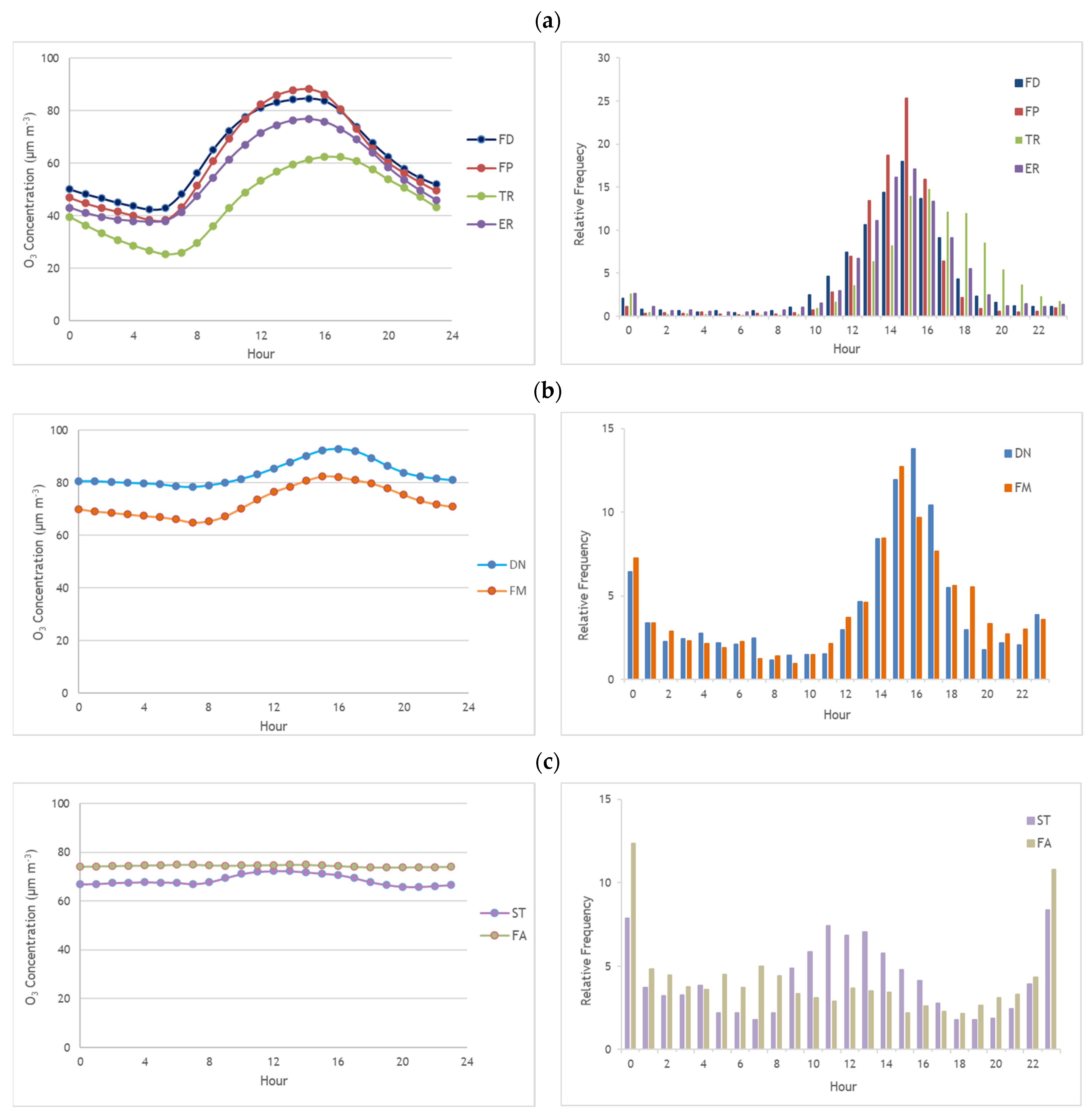
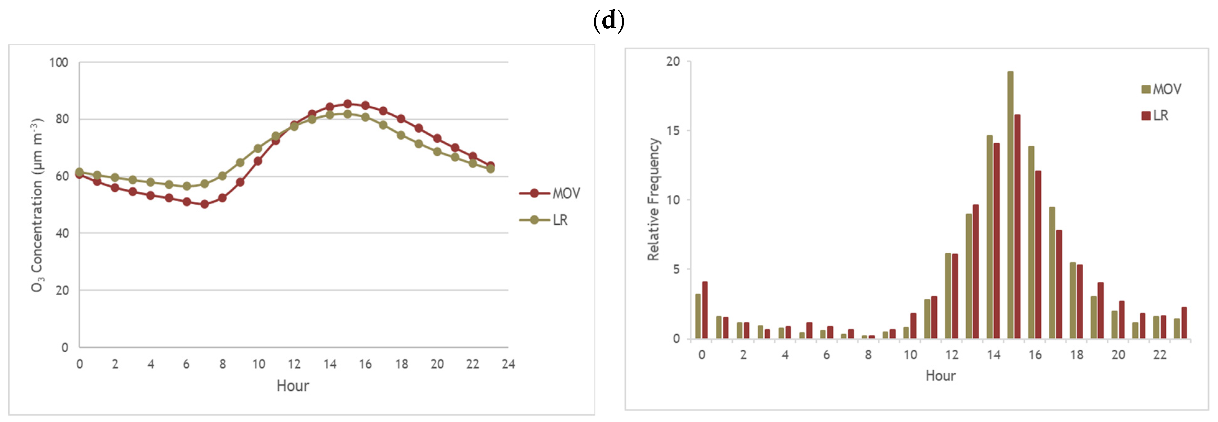
The daily average ozone concentration profiles (in μm m−3) and the relative frequency (in percentage) of its maximum for the first four clusters are shown in Figure 6. The first cluster shows stations with a higher variation in the O3 concentration during the day, presenting a decrease in the early morning followed by an increase in the afternoon, with most having their peak at 15 h, as shown in the maximum concentrations profile. In cluster 2, O3 concentrations have similar behaviours, increasing between 15 h and 16 h. The O3 concentrations show higher values (and reduced amplitude of values) than those observed in the previous cluster. The stations representing the Portuguese Islands are grouped in cluster 3. They show the lowest concentrations and the shortest variation between the daily minimum and maximum. In the final cluster, the ozone profile in both stations is closer to cluster 1; however, the daily maximum and minimum are lower. Except for stations in cluster 3, a similar daily profile of O3 concentration was observed in all monitoring stations, the lowest occurring in the morning and the highest in the early afternoon. In FA and ST stations, the peak occurs at night. This event results from the horizontal and vertical transport of ozone and its precursors [13]. Studies of nocturnal ozone concentration increase were developed in the Portuguese continent to explain unexpected ozone levels [21,36]. The ozone enhancement events can be related to transport processes and the related usual meteorological conditions due to the absence of photochemical production. Additionally, vertical mixing was registered in the boundary layer in winter, contributing to surface nocturnal ozone peaks.
3.2. Surface Ozone and NOx Relation
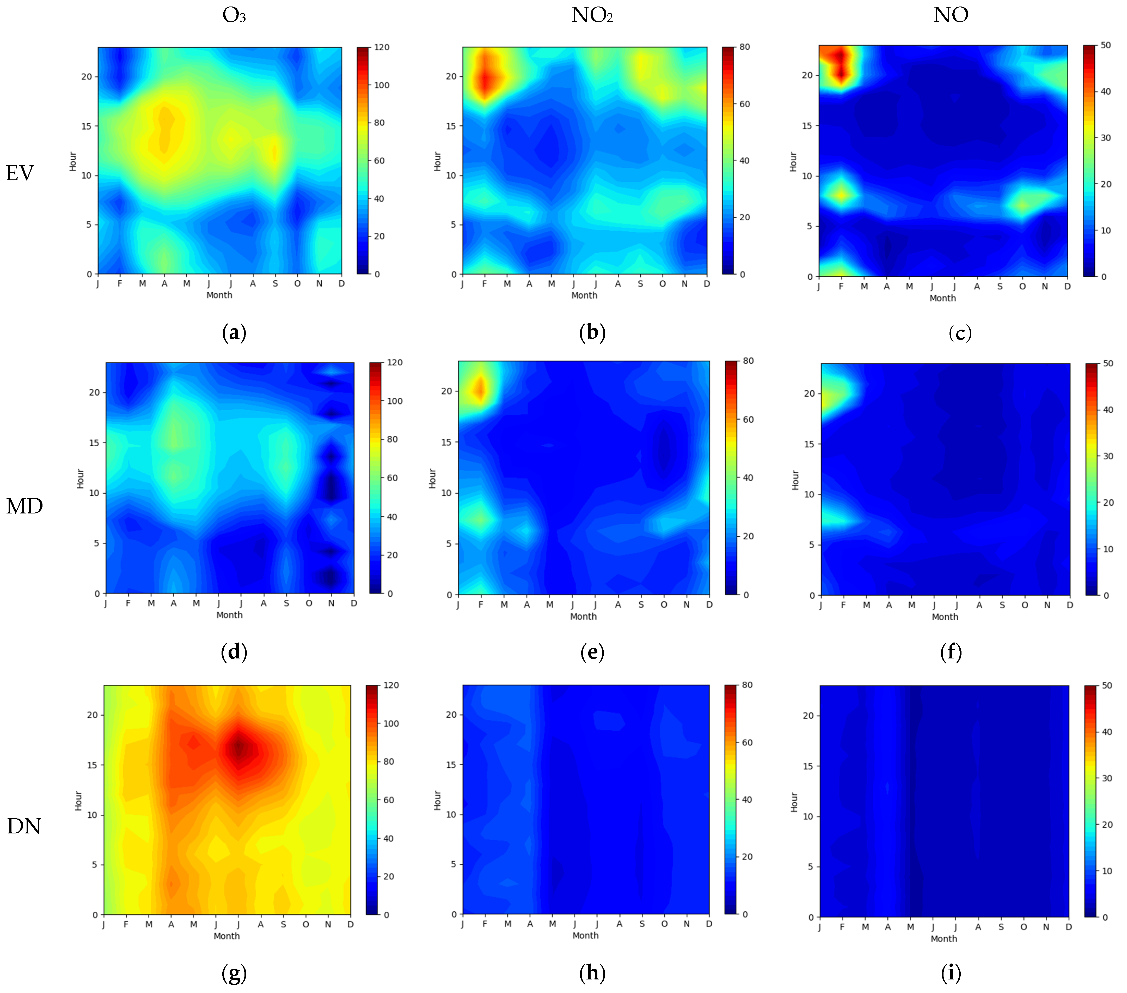
In suburban and urban areas, surface O3 concentrations are lower than at rural sites. Figure 7 presents O3, NO2, and NO daily average concentrations for the EV, MD, and DN stations in different months. High O3 concentrations in the DN station can be observed compared with the other two stations. For all stations, high concentrations were observed in the afternoon. As for NO2 and NO, the concentrations were expectably higher in the suburban and urban areas due to more intensive anthropogenic emission rates. High values observed in the first hours of the day (especially in the NO2 plot) can be explained by the lack of ozone formation during this period. As expected, the anthropogenic influence in rural stations is weaker, shown by lower levels of NOx in the DN station (Figure 7h,i). In general, an almost-symmetric daily profile is shown between O3 and NOx: in the first hours of the day, NOx levels are low due to low emissions; in the morning, with the beginning of anthropogenic activities (specifically traffic emissions), there is an increase in NO and NO2 emissions followed by a decrease in ozone levels due to titration with NO; and during the afternoon, when there is a greater incidence of solar radiation, the NO2 emitted and formed through the NO present in the air will lead to ozone formation. In the nighttime, ozone levels usually decrease due to the lack of solar radiation. In these conditions, NO2 photolysis does not occur, and the existing NO can be oxidised back to NO2 with the reaction with O3.
Ferreira et al. [37] presented the same connection between O3 and NO2 levels in the Lisbon region, registering a higher ozone concentration in the periphery of the urban centre. In the southwest of the Iberian Peninsula, a study of O3, NO, and NO2 trends was developed at rural, urban, suburban, and industrial sites by Domínguez-López et al. [10]. According to their reports, most rural sites presented a low and constant NOx level. In suburban and urban stations, besides the morning NOx peak, there is a second in the evening due to a decrease in solar activity and an increase in traffic. In the same reference, an analysis of monthly variations showed similar results to the ones shown in Figure 7, with higher ozone levels in the spring and summer for all stations and NOx levels higher in the autumn and winter for urban and suburban sites, while NO2 and NO at steady levels during the year were observed at rural sites. In Spain, urban/suburban sites also registered higher NO and NO2 concentrations and O3 higher levels in rural/remote regions [35], as shown in a study conducted in the UK too [38].
Considering the ozone concentrations at a chemical equilibrium state, that is, a relation to the NO2/NO ratio (Equation (2), being K the equilibrium constant),
[O3] = [NO2]·[O2]/[NO]·K,
Thus, the influence of the NO2/NO ratio in the O3 concentration was also included in the PC and MLR analysis. A correlation matrix was obtained (Table 4, Table 5 and Table 6) to demonstrate the relationship between ozone and its considered precursors in 2019.
Considering the strength of variables association (see Table S2), Table 4 presents a significant negative correlation between O3, NO2, and NO and a medium positive association with NO2/NO in the urban station (EV), which is what was expected for this type of environment. These results confirm the previous logic of the anti-correlation of ozone and its precursor’s daily profile, particularly noticed in the urban sites. Regarding the combined effect of the selected environmental variables, MLR identified a negative relation between NO2 and O3 concentrations and a positive with NO, trends also known in other studies in the literature [39].
In the suburban sites (Table 5), a weaker relationship between O3 and NOx is expected than in the urban site (Figure 7b). The PC coefficients for O3 and its precursors obtained are lower than those for the EV station. The NO shows a small correlation with O3, and the NO2/NO ratio shows no correlation (coefficient value close to 0). That result is also shown in the smaller b3 value of MLR, compared to the previous value. The NO2 shows a small negative association with O3 and does not show statistical significance to its formation, according to the MLR analysis (b1 was not considered statistically significant). Table 6 shows the PC and MLR results for the DN station. As is expected, the rural site shows a low (NO2 and NO) or no relation (NO2/NO ratio) between O3 and its chemical precursors. According to the MLR results, NO2 levels do not influence ozone formation at this site. Contrary to the suburban station, the NO concentration and NO2/NO ratio have a small negative effect on O3 levels.
The strength of the association varies with season [40]. The correlation analysis in each season showed negative correlations of O3 with NO and NO2 (higher correlation with NO2 in spring and summer and with NO in the autumn and winter) [41]. This difference can be explained by the interference of meteorological parameters and distinct weather types that affect the pollutants’ transport and mixing in the atmosphere.
3.3. Surface Ozone and Meteorological Parameters Relation
The permanence of pollutants in the atmosphere is not only affected by chemical reactions among themselves but also by meteorological conditions, whether at a micro or macro scale. Studying the weather conditions when peak pollutant levels are registered is important to prevent negative effects on humans and the ecosystem. The ozone formation is enhanced by solar radiation and other meteorological parameters. Since these have different levels throughout the year, a quarterly analysis was performed applying PC and MLR to O3 and the meteorological parameters considered (Table 7 and Table 8). The stations under analysis are suburban-type, located in sites with relative anthropogenic influence (e.g., the city airport-related activities). In the MP station, the first quarter presented a medium- (between 0.3 and 0.5) positive correlation with temperature (T) and solar radiation (SR) and a small negative association with relative humidity (RH), meaning that the increase in RH leads to a decrease in ozone (disregarding the results not statistically significant). The MLR, on the contrary, points to a small influence of pressure (P) in the ozone concentration, and relative humidity does not play a role in ozone formation/elimination. A small negative correlation of P and O3 is pointed to in the second quarter, agreeing with the b1 value for that period. T and SR show a continuous significant correlation (also seen in the 3rd and 4th quarters). The RH shows stronger negative correlations in the spring and summer seasons. According to MLR results, the SR has a greater impact in the April–May–June period than the October–November–December period. RH shows a significant negative relation with ozone in the 3rd quarter, and, in the same period, T does not influence O3 levels.
In the VNT station, P presents a higher correlation with ozone in the 4th quarter. The MLR results also show a negative influence of P on ozone levels. In this station, the correlation of T and O3 presents stronger values, and, except in the 3rd quarter, there is a similar influence level of T in O3 concentrations. The RH presents a high PC coefficient, but the MLR analysis shows only this parameter influence in the 2nd and 3rd quarters. As for SR, there is a positive correlation with high coefficient values. Ferreira et al. [37] studied the relationship between ozone and some parameters in Lisbon city. Accordingly, daily sea level medium pressure and medium relative humidity negatively influence ozone production in all seasons. As for temperature, the daily medium value only shows a positive (and weak) correlation in the winter months. Pires et al. [24] showed a weak positive correlation of T and a slight negative association of SR and RH with O3 in a station located in Northern Portugal. The discrepancies between the two applied statistical methods expose the complex task of predicting ozone levels, although, in general, studies applying relationship methods show a positive correlation of O3 with SR and T and a negative correlation with RH [39,41].
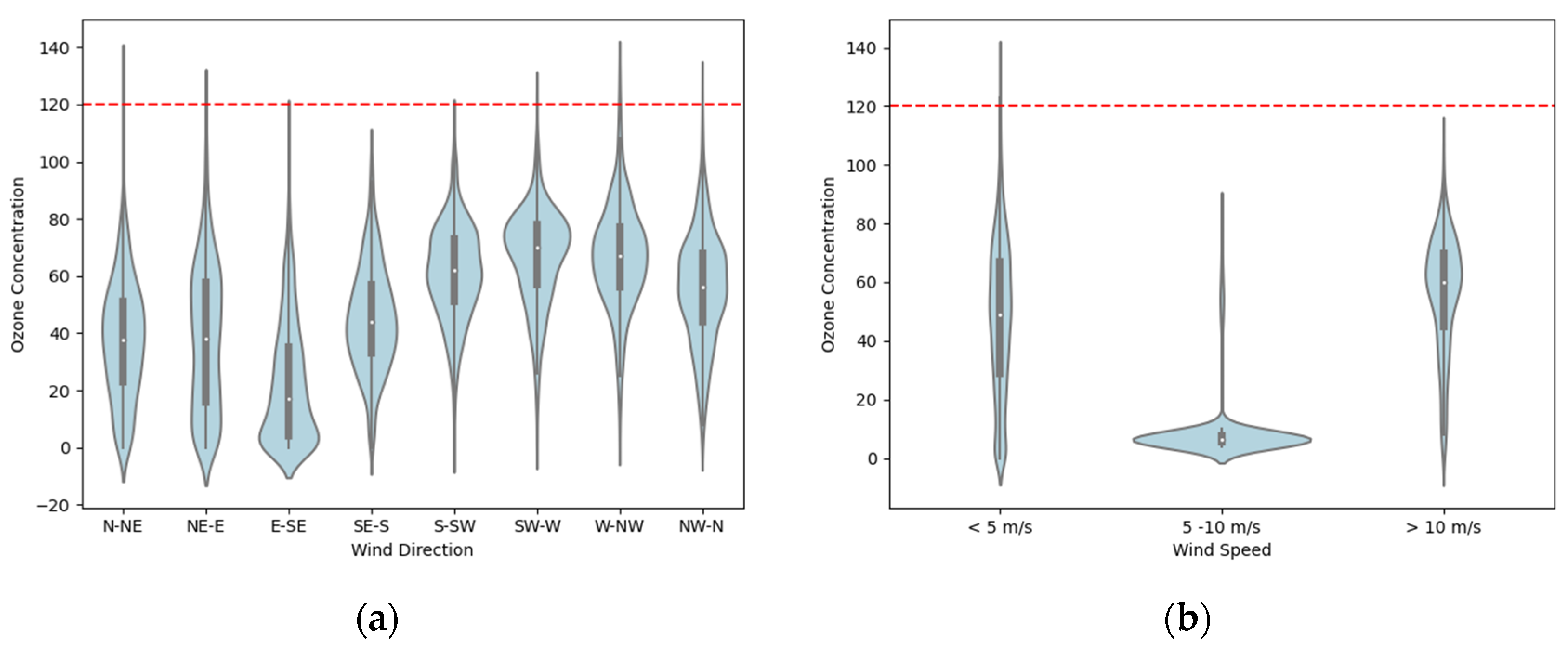
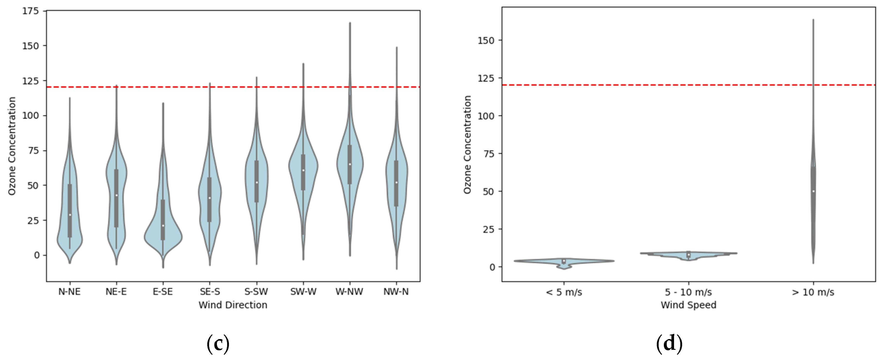
O3 concentrations can also be influenced by transport and mixing phenomena. Thus, an analyse relating wind direction and speed with O3 was implemented. Figure S4 presents a wind rose with the wind speed and direction distribution for the year 2015. The most prominent winds were from NW (stronger winds) and E (calmer winds) related to the air masses from the Atlantic Ocean and Spain that the northern Portuguese region is subjected to. On a macro scale (synoptic weather), it is essential to mention the influence of the Azores anticyclone in Europe [42,43,44], especially in the Mediterranean [25,35,45,46,47,48]. This type of weather system is related to a higher T and low RH and cloud cover (consequently contributing to higher SR activity), enhancing O3 production. The relatively low wind activity provides the accumulation of this pollutant in the atmosphere.
A more significant contribution of air masses from the Atlantic Ocean for ozone higher concentrations is observed (median values represented in the violin plots, Figure 8). The peak O3 values are registered for the N-NE and W-NW directions in the MP station. Located closer to shore, the higher concentrations are registered when the wind has lower speed values (more calm weather), which allows the accumulation of ozone. In the VNT station, the peak levels are reached under the North Atlantic air masses influence (NW-N). They are related to faster wind activity, possibly meaning that the high ozone concentrations in this site are associated with the circulation of polluted air masses. Santurtún et al. [48] related ozone trends to weather types in Spain. Accordingly, the stations studied were influenced by the anticyclone system and east and northeast flow (corresponding to the information in Figure S4). Knowing the comparable importance of both chemical and meteorological precursors to ozone formation, Li et al. [49] studied the increase of O3 pollution in China, concluding that temperature is the meteorological parameter with more influence, but that it is related to anticyclonic conditions. Additionally, the authors pointed to the decrease in PM2.5 and the unmitigated emissions of VOCs from anthropogenic sources.
4. Conclusions
Annual average O3 concentrations presented a decreasing trend during the analysed period. However, exceedances to EU legislated values for human health protection were still observed. CA identified several O3 concentration patterns, showing the effectiveness of the current geographical distribution of the air quality monitoring stations. Negative correlations were determined between NO, NO2, and O3 concentrations in urban and suburban stations. The correlation with the NO2/NO ratio only showed significance in the urban site. As for MLR results, in general, the stronger influence of NOx levels was expected in the urban station. The O3 concentrations in both suburban sites showed a strong positive correlation between O3, T, and SR, a strong negative correlation with RH, and a weaker negative association with pressure. The meteorological parameter that shows a higher contribution in O3 concentration was solar radiation, showing a stronger influence in the 2nd annual quarter, where the spring high average concentrations are registered. The wind direction distribution showed that the location was under the flow of NW and E-SE winds, related to the Azores anticyclone, and air masses from the Iberian Peninsula, inland.
Supplementary Materials
The following supporting information can be downloaded at: https://www.mdpi.com/article/10.3390/su14042383/s1, Figure S1: Map with the geographical distribution of Portugal’s rural monitoring stations; Figure S2A: Dendrograms for years (a) 2009, (b) 2010, (c) 2011, (d) 2013, (e) 2014 and (f) 2015; Figure S2B: Dendrograms for years (a) 2016, (b) 2017, (c) 2018 and (d) 2019; Figure S3: Annual profile of O3 concentration (μg m−3) and monthly distribution for 2012 at different stations: (a) Douro-Norte; (b) Fundão; (c) Fernando Pó; (d) Faial; Figure S4: Wind rose with wind direction and speed distribution for the year 2015; Table S1: Matrix of relative frequencies depicting the relationship between the different stations; and Table S2: Guidelines for interpretation of PC coefficient values [50].
Author Contributions
Conceptualisation, J.C.M.P.; Methodology, R.C.V.S. and J.C.M.P.; Software, R.C.V.S. and J.C.M.P.; Validation, R.C.V.S. and J.C.M.P.; Formal Analysis, R.C.V.S. and J.C.M.P.; Investigation, R.C.V.S. and J.C.M.P.; Data Curation, R.C.V.S. and J.C.M.P.; Writing—Original Draft Preparation, R.C.V.S.; Writing—Review and Editing, R.C.V.S. and J.C.M.P.; Visualization, R.C.V.S. and J.C.M.P.; Supervision, J.C.M.P.; Funding Acquisition, J.C.M.P. All authors have read and agreed to the published version of the manuscript.
Funding
This work was financially supported by: LA/P/0045/2020 (ALiCE) and UIDB/00511/2020-UIDP/00511/2020 (LEPABE) funded by national funds through FCT/MCTES (PIDDAC). J.C.M.P. acknowledges the FCT Investigator 2015 Programme (IF/01341/2015).
Institutional Review Board Statement
Not applicable.
Informed Consent Statement
Not applicable.
Acknowledgments
The authors thank Instituto Português do Mar e da Atmosfera (IPMA) for providing the meteorological data.
Conflicts of Interest
The authors declare no conflict of interest.
References
- Seinfeld, J.H.; Pandis, S.N. Atmospheric Chemistry and Physics: From Air Pollution to Climate Change; John Wiley & Sons, Inc.: Hoboken, NJ, USA, 1998. [Google Scholar]
- Sousa, S.I.; Ferraz, M.A.; Pereira, M.C.; Martins, F.G. Avaliação das Concentrações Pré-industriais e Actuais de Ozono Superficial através de Séries Temporais. In Proceedings of the 8ª Conferência Nacional de Ambiente, Lisboa, Portugal, 27–29 October 2004. [Google Scholar]
- Wallace, J.M.; Hobbs, P.V. Atmospheric Science—An Introductory Survay; Elsevier: Amsterdam, The Netherlands, 2006. [Google Scholar]
- EEA. Air quality in Europe—2020 Report; EEA: Copenhagen, Denmark, 2020. [Google Scholar]
- EEA. Exposure of Europe’s Ecosystems to Ozone. Available online: https://www.eea.europa.eu/api/SITE/data-and-maps/indicators/exposure-of-ecosystems-to-acidification-15 (accessed on 4 June 2021).
- Pleijel, H.; Broberg, M.C.; Uddling, J.; Mills, G. Current surface ozone concentrations significantly decrease wheat growth, yield and quality. Sci. Total Environ. 2018, 613, 687–692. [Google Scholar] [CrossRef] [PubMed]
- Feng, Z.; De Marco, A.; Anav, A.; Gualtieri, M.; Sicard, P.; Tian, H.; Fornasier, F.; Tao, F.; Guo, A.; Paoletti, E. Economic losses due to ozone impacts on human health, forest productivity and crop yield across China. Environ. Int. 2019, 131, 104966. [Google Scholar] [CrossRef] [PubMed]
- Finlayson-Pitts, B.J.; Pitts, J.N. Atmospheric chemistry of tropospheric ozone formation: Scientific and regulatory implications. Air Waste 1993, 43, 1091–1100. [Google Scholar] [CrossRef]
- Li, K.; Jacob, D.; Liao, H.; Shen, L.; Zhang, Q.; Bates, K. Anthropogenic drivers of 2013–2017 trends in summer surface ozone in China. Proc. Natl. Acad. Sci. USA 2019, 116, 422–427. [Google Scholar] [CrossRef] [PubMed] [Green Version]
- Domínguez-López, D.; Adame, J.A.; Hernández-Ceballos, M.A.; Vaca, F.; De La Morena, B.A.; Bolívar, J.P. Spatial and temporal variation of surface ozone, NO and NO2 at urban, suburban, rural and industrial sites in the southwest of the Iberian Peninsula. Environ. Monit. Assess. 2014, 186, 5337–5351. [Google Scholar] [CrossRef] [PubMed]
- Sun, H.; Shin, Y.; Xia, M.; Ke, S.; Yuan, L.; Guo, Y.; Archibald, A. Spatial Resolved Surface Ozone with Urban and Rural Differentiation during 1990–2019: A Space-Time Bayesian Neural Network Downscaler. Environ. Sci. Technol. 2021, 5, 167–174. [Google Scholar] [CrossRef] [PubMed]
- Notario, A.; Díaz-de-Mera, Y.; Aranda, A.; Adame, J.A.; Parra, A.; Romero, E.; Parra, J.; Muñoz, F. Surface ozone comparison conducted in two rural areas in central-southern Spain. Environ. Sci. Pollut. Res. 2012, 19, 186–200. [Google Scholar] [CrossRef]
- Pires, J.C.M.; Alvim-Ferraz, M.C.M.; Martins, F.G. Surface ozone behaviour at rural sites in Portugal. Atmos. Res. 2012, 104–105, 164–171. [Google Scholar] [CrossRef]
- Charlson, R.; Schwartz, S.; Hales, J.; Cess, R.; Coakley, J.A., Jr.; Hansen, J.; Hofmann, D. Climate Forcing by Anthropogenic Aerosols. Science 1992, 255, 423–430. [Google Scholar] [CrossRef]
- Lou, S.; Liao, H.; Zhu, B. Impacts of aerosols on surface-layer ozone concentrations in China through heterogeneous reactions and changes in photolysis rates. Atmos. Environ. 2014, 85, 123–138. [Google Scholar] [CrossRef]
- Fang, C.; Wang, L.; Wang, J. Analysis of the spatial–temporal variation of the surface ozone concentration and its associated meteorological factors in Changchun. Environments 2019, 6, 46. [Google Scholar] [CrossRef] [Green Version]
- Afonso, N.F.; Pires, J.C.M. Characterization of surface ozone behavior at different regimes. Appl. Sci. 2017, 7, 944. [Google Scholar] [CrossRef] [Green Version]
- Barros, N.; Silva, M.P.; Fontes, T.; Manso, M.C.; Carvalho, A.C. Learning from 24 years of ozone data in Portugal. WIT Trans. Ecol. Environ. 2014, 183, 117–128. [Google Scholar] [CrossRef] [Green Version]
- Fernández-Guisuraga, J.M.; Castro, A.; Alves, C.; Calvo, A.; Alonso-Blanco, E.; Blanco-Alegre, C.; Rocha, A.; Fraile, R. Nitrogen oxides and ozone in Portugal: Trends and ozone estimation in an urban and a rural site. Environ. Sci. Pollut. Res. 2016, 23, 17171–17182. [Google Scholar] [CrossRef] [PubMed]
- Kulkarni, P.S.; Bortoli, D.; Domingues, A.; Silva, A.M. Surface ozone variability and trend over urban and suburban sites in Portugal. Aerosol Air Qual. Res. 2016, 16, 138–152. [Google Scholar] [CrossRef] [Green Version]
- Kulkarni, P.S.; Bortoli, D.; Silva, A.M. Nocturnal surface ozone enhancement and trend over urban and suburban sites in Portugal. Atmos. Environ. 2013, 71, 251–259. [Google Scholar] [CrossRef]
- Borrego, C.; Monteiro, A.; Martins, H.; Ferreira, J.; Fernandes, A.P.; Rafael, S.; Miranda, A.I.; Guevara, M.; Baldasano, J.M. Air quality plan for ozone: An urgent need for North Portugal. Air Qual. Atmos. Health 2016, 9, 447–460. [Google Scholar] [CrossRef]
- Pires, J.C.M.; Gonçalves, B.; Azevedo, F.G.; Carneiro, A.P.; Rego, N.; Assembleia, A.J.B.; Lima, J.F.B.; Silva, P.A.; Alves, C.; Martins, F.G. Optimization of artificial neural network models through genetic algorithms for surface ozone concentration forecasting. Environ. Sci. Pollut. Res. 2012, 19, 3228–3234. [Google Scholar] [CrossRef]
- Pires, J.C.M.; Martins, F.G.; Sousa, S.I.V.; Alvim-Ferraz, M.C.M.; Pereira, M.C. Selection and validation of parameters in multiple linear and principal components regression. Environ. Model. Softw. 2008, 7, 50–55. [Google Scholar] [CrossRef]
- Carvalho, A.; Monteiro, A.; Ribeiro, I.; Tchepel, O.; Miranda, A.I.; Borrego, C.; Saavedra, S.; Souto, J.A.; Casares, J.J. High ozone levels in the northeast of Portugal: Analysis and characterization. Atmos. Environ. 2010, 44, 1020–1031. [Google Scholar] [CrossRef]
- Monteiro, A.; Gouveia, S.; Scotto, M.G.; Lopes, J.; Gama, C.; Feliciano, M.; Miranda, A.I. Investigating ozone episodes in Portugal: A wavelet-based approach. Air Qual. Atmos. Health 2016, 9, 775–783. [Google Scholar] [CrossRef] [Green Version]
- QualAR. Dados Estações. Available online: https://qualar.apambiente.pt/downloads (accessed on 8 January 2021).
- Diário da República. Decreto-Lei nº 102/2010; Diário da República Electrónico: Lisbon, Portugal, 2010; pp. 4177–4205. [Google Scholar]
- Afonso, P.A.F. Concentrações de Ozono Superficial em Portugal: Avaliação dos Padrões Temporais e dos Contrastes Espaciais em Estações de Fundo; Instituto Politécnico de Bragança: Bragança, Portugal, 2014. [Google Scholar]
- Yan, Y.; Pozzer, A.; Ojha, N.; Lin, J.; Lelieveld, J. Analysis of European ozone trends in the period 1995. Atmos. Chem. Phys. 2018, 18, 5589–5605. [Google Scholar] [CrossRef] [Green Version]
- Chang, K.L.; Petropavlovskikh, I.; Cooper, O.R.; Schultz, M.G.; Wang, T. Regional trend analysis of surface ozone observations from monitoring networks in eastern North America, Europe and East Asia. Elementa 2017, 5, 5. [Google Scholar] [CrossRef] [Green Version]
- Proietti, C.; Fornasier, M.F.; Sicard, P.; Anav, A.; Paoletti, E.; De Marco, A. Trends in tropospheric ozone concentrations and forest impact metrics in Europe over the time period 2000. J. For. Res. 2021, 32, 543–551. [Google Scholar] [CrossRef]
- Luo, J.; Liang, W.; Xu, P.; Xue, H.; Zhang, M.; Shang, L.; Tian, H. Seasonal Features and a Case Study of Tropopause Folds over the Tibetan Plateau. Adv. Meteorol. 2019, 2019, 4375123. [Google Scholar] [CrossRef]
- Vingarzan, R. A review of surface ozone background levels and trends. Atmos. Environ. 2004, 38, 3431–3442. [Google Scholar] [CrossRef]
- Massagué, J.; Contreras, J.; Campos, A.; Alastuey, A.; Querol, X. 2005–2018 trends in ozone peak concentrations and spatial contributions in the Guadalquivir Valley, southern Spain. Atmos. Environ. 2021, 254, 118385. [Google Scholar] [CrossRef]
- Kulkarni, P.S.; Dasari, H.P.; Sharma, A.; Bortoli, D.; Salgado, R.; Silva, A.M. Nocturnal surface ozone enhancement over Portugal during winter: Influence of different atmospheric conditions. Atmos. Environ. 2016, 147, 109–120. [Google Scholar] [CrossRef] [Green Version]
- Ferreira, F.C.; Torres, P.M.; Tente, H.S.; Neto, J.B. Ozone levels in Portugal: The Lisbon region assessment. In Proceedings of the Air and Waste Management Association’s Annual Conference and Exhibition, AWMA, Indianapolis, IN, USA, 22–25 June 2004. [Google Scholar]
- Finch, D.P.; Palmer, P.I. Increasing ambient surface ozone levels over the UK accompanied by fewer extreme events. Atmos. Environ. 2020, 237, 117627. [Google Scholar] [CrossRef]
- Mazzuca, G.M.; Pickering, K.E.; New, D.A.; Dreessen, J.; Dickerson, R.R. Impact of bay breeze and thunderstorm circulations on surface ozone at a site along the Chesapeake Bay 2011. Atmos. Environ. 2019, 198, 351–365. [Google Scholar] [CrossRef]
- Venkanna, R.; Nikhil, G.N.; Siva Rao, T.; Sinha, P.R.; Swamy, Y.V. Environmental monitoring of surface ozone and other trace gases over different time scales: Chemistry, transport and modeling. Int. J. Environ. Sci. Technol. 2015, 12, 1749–1758. [Google Scholar] [CrossRef]
- Paraschiv, S.; Barbuta-Misu, N.; Paraschiv, S.L. Influence of NO2, NO and meteorological conditions on the tropospheric O3 concentration at an industrial station. Energy Rep. 2020, 6, 231–236. [Google Scholar] [CrossRef]
- Katragkou, E.; Zanis, P.; Tegoulias, I.; Melas, D.; Kioutsioukis, I.; Küger, B.C.; Huszar, P.; Halenka, T.; Rauscher, S. Decadal regional air quality simulations over Europe in present climate: Near surface ozone sensitivity to external meteorological forcing. Atmos. Chem. Phys. 2010, 10, 11805–11821. [Google Scholar] [CrossRef] [Green Version]
- Pope, R.J.; Butt, E.W.; Chipperfield, M.P.; Doherty, R.M.; Fenech, S.; Schmidt, A.; Arnold, S.R.; Savage, N.H. The impact of synoptic weather on UK surface ozone and implications for premature mortality. Environ. Res. Lett. 2016, 11, 124004. [Google Scholar] [CrossRef] [Green Version]
- Solberg, S.; Derwent, R.G.; Hov, Ø.; Langner, J.; Lindskog, A. European abatement of surface ozone in a global perspective. Ambio 2005, 34, 47–53. [Google Scholar] [CrossRef]
- Adame, J.A.; Lozano, A.; Bolívar, J.P.; De la Morena, B.A.; Contreras, J.; Godoy, F. Behavior, distribution and variability of surface ozone at an arid region in the south of Iberian Peninsula (Seville, Spain). Chemosphere 2008, 70, 841–849. [Google Scholar] [CrossRef]
- Carnero, J.A.A.; Bolívar, J.P.; de la Morena, B.A. Surface ozone measurements in the southwest of the Iberian Peninsula (Huelva, Spain). Environ. Sci. Pollut. Res. 2010, 17, 355–368. [Google Scholar] [CrossRef]
- Kalabokas, P.D.; Mihalopoulos, N.; Ellul, R.; Kleanthous, S.; Repapis, C.C. An investigation of the meteorological and photochemical factors influencing the background rural and marine surface ozone levels in the Central and Eastern Mediterranean. Atmos. Environ. 2008, 42, 7894–7906. [Google Scholar] [CrossRef]
- Santurtún, A.; González-Hidalgo, J.C.; Sanchez-Lorenzo, A.; Zarrabeitia, M.T. Surface ozone concentration trends and its relationship with weather types in Spain (2001–2010). Atmos. Environ. 2015, 101, 10–22. [Google Scholar] [CrossRef]
- Li, K.; Jacob, D.J.; Shen, L.; Lu, X.; De Smedt, I.; Liao, H. Increases in surface ozone pollution in China from 2013 to 2019: Anthropogenic and meteorological influences. Atmos. Chem. Phys. 2020, 20, 11423–11433. [Google Scholar] [CrossRef]
- Statistics, L. Pearson’s Product Moment Correlation. Statistical Tutorials and Software Guides 2020. Available online: https://statistics.laerd.com/statistical-guides/pearson-correlation-coefficient-statistical-guide.php (accessed on 12 June 2021).
Figure 1.
Geographical distribution of O3 monitoring stations EV (urban), MD (suburban), and DN (rural).
Figure 1.
Geographical distribution of O3 monitoring stations EV (urban), MD (suburban), and DN (rural).

Figure 2.
Geographical distribution of the meteorological station (EMA) and O3 monitoring stations, MP and VNT.
Figure 2.
Geographical distribution of the meteorological station (EMA) and O3 monitoring stations, MP and VNT.

Figure 3.
O3 annual average concentration in each of Portugal’s most important regions: (a) Regions of North and Centre; (b) Regions of Lisbon and Tejo Valley and Alentejo; (c) Regions of Algarve and Islands.
Figure 3.
O3 annual average concentration in each of Portugal’s most important regions: (a) Regions of North and Centre; (b) Regions of Lisbon and Tejo Valley and Alentejo; (c) Regions of Algarve and Islands.

Figure 4.
AOT40 levels in each station in the study period.

Figure 5.
Dendrogram obtained from cluster analysis for 2012.

Figure 6.
Daily average O3 concentration profile (on the left) and daily evolution of the relative frequency (in percentage) of the daily maximum O3 concentration for the analysed period (on the right), for cluster 1 (a), cluster 2 (b), cluster 3 (c) and cluster 4 (d).
Figure 6.
Daily average O3 concentration profile (on the left) and daily evolution of the relative frequency (in percentage) of the daily maximum O3 concentration for the analysed period (on the right), for cluster 1 (a), cluster 2 (b), cluster 3 (c) and cluster 4 (d).


Figure 7.
Contour plot of O3 (a,d,g), NO2 (b,e,h), and NO (c,f,i) concentrations (in μg m−3) at EV (urban), MD (suburban), and DN (rural) stations.
Figure 7.
Contour plot of O3 (a,d,g), NO2 (b,e,h), and NO (c,f,i) concentrations (in μg m−3) at EV (urban), MD (suburban), and DN (rural) stations.

Figure 8.
Relationship between wind direction and speed with ozone levels (in μm m−3) at (a,b) MP and (c,d) VNT stations.
Figure 8.
Relationship between wind direction and speed with ozone levels (in μm m−3) at (a,b) MP and (c,d) VNT stations.


Table 1.
Geographical coordinates, altitude, and minimum distance to the seashore of the existing rural sites.
Table 1.
Geographical coordinates, altitude, and minimum distance to the seashore of the existing rural sites.
| Monitoring Stations | Geographical Coordinates | Altitude (m) | Minimum Distance to the Seashore (km) | |
|---|---|---|---|---|
| CH | Chamusca | 39°21′15″ N 08°28′03″ W | 143 | 58.5 |
| CR | Cerro | 37°18′45″ N 07°40′43″ W | 300 | 21.1 |
| DN | Douro Norte | 41°22′17″ N 07°47′27″ W | 1086 | 78.4 |
| ER | Ervedeira | 39°55′28″ N 08°53′34″ W | 68 | 4.5 |
| FA | Faial | 38°36′18″ N 28°37′53″ W | 310 | 0.7 |
| FD | Fundão | 40°13′59″ N 07°17′58″ W | 461 | 133.6 |
| FM | Fornelo do Monte | 40°38′39″ N 08°06′00″ W | 731 | 53.4 |
| FP | Fernando Pó | 38°38′14″ N 08°41′30″ W | 57 | 25.2 |
| LR | Lourinhã | 39°16′48″ N 09°14′04″ W | 143 | 7.6 |
| ML | Minho-Lima | 41°48′08″ N 08°41′38″ W | 777 | 14.2 |
| MOV | Montemor-o-Velho | 40°12′08″ N 08°40′08″ W | 14 | 17.9 |
| MV | Monte Velho | 38°04′37″ N 08°47′55″ W | 53 | 1.2 |
| SN | Sonega | 37°52′16″ N 08°43′26″ W | 235 | 1.4 |
| ST | Santana | 32°48′28″ N 16°53′11″ W | 0 | 125.1 |
| TR | Terena | 38°36′54″ N 07°23′51″ W | 187 | 125.1 |
Table 2.
Air quality monitoring efficiency (in percentage) for rural stations.
| CH | CR | DN | ER | FA | FD | FM | FP | LR | ML | MOV | MV | SN | ST | TR | |
|---|---|---|---|---|---|---|---|---|---|---|---|---|---|---|---|
| 2009 | 94 | 0 | 84 | 96 | 44 | 99 | 95 | 99 | 94 | 89 | 94 | 0 | 99 | 0 | 97 |
| 2010 | 100 | 19 | 83 | 99 | 89 | 96 | 97 | 98 | 0 | 56 | 99 | 0 | 99 | 0 | 93 |
| 2011 | 100 | 40 | 86 | 100 | 98 | 99 | 94 | 96 | 98 | 67 | 100 | 0 | 100 | 0 | 92 |
| 2012 | 99 | 99 | 96 | 95 | 91 | 100 | 99 | 99 | 98 | 100 | 99 | 0 | 86 | 0 | 100 |
| 2013 | 99 | 87 | 94 | 90 | 98 | 100 | 98 | 93 | 89 | 97 | 92 | 0 | 88 | 0 | 100 |
| 2014 | 93 | 88 | 82 | 99 | 94 | 99 | 96 | 91 | 94 | 30 | 99 | 0 | 100 | 0 | 100 |
| 2015 | 99 | 97 | 27 | 99 | 99 | 84 | 90 | 100 | 98 | 12 | 99 | 96 | 57 | 0 | 94 |
| 2016 | 98 | 89 | 25 | 97 | 93 | 98 | 98 | 99 | 96 | 18 | 68 | 62 | 99 | 99 | 99 |
| 2017 | 98 | 88 | 54 | 99 | 100 | 99 | 74 | 98 | 98 | 0 | 100 | 0 | 93 | 100 | 99 |
| 2018 | 97 | 94 | 98 | 52 | 99 | 97 | 83 | 98 | 100 | 59 | 78 | 50 | 0 | 100 | 92 |
| 2019 | 91 | 95 | 90 | 0 | 100 | 92 | 94 | 100 | 94 | 59 | 0 | 0 | 0 | 100 | 91 |
Table 3.
Exceedances to O3 alert threshold (AT), information threshold (IT), and target value (TV) for human health protection.
Table 3.
Exceedances to O3 alert threshold (AT), information threshold (IT), and target value (TV) for human health protection.
| CH | CR | DN | ER | FA | FD | FM | FP | LR | ML | MOV | SN | ST | TR | ||
|---|---|---|---|---|---|---|---|---|---|---|---|---|---|---|---|
| 2009 | AT | 0 | - | 3 | 0 | - | 0 | 0 | 0 | 0 | 0 | 0 | 0 | - | 0 |
| IT | 3 | - | 37 | 9 | - | 0 | 11 | 4 | 0 | 0 | 1 | 0 | - | 0 | |
| TV | 57 | - | 76 | 21 | - | 33 | 48 | 32 | 19 | 0 | 24 | 0 | - | 0 | |
| 2010 | AT | 0 | - | 4 | 0 | 0 | 0 | 1 | 0 | - | - | 0 | 0 | - | 0 |
| IT | 16 | - | 76 | 8 | 0 | 3 | 36 | 1 | - | - | 9 | 0 | - | 0 | |
| TV | 55 | - | 66 | 29 | 2 | 31 | 66 | 37 | - | - | 26 | 0 | - | 0 | |
| 2011 | AT | 0 | - | 0 | 0 | 0 | 0 | 0 | 0 | 0 | - | 0 | 0 | - | 0 |
| IT | 4 | - | 30 | 0 | 0 | 0 | 1 | 7 | 0 | - | 3 | 0 | - | 0 | |
| TV | 38 | - | 67 | 0 | 0 | 15 | 2 | 27 | 19 | - | 53 | 0 | - | 0 | |
| 2012 | AT | 0 | 0 | 0 | 0 | 0 | 0 | 0 | 0 | 0 | 0 | 0 | 0 | - | 0 |
| IT | 4 | 0 | 16 | 0 | 0 | 0 | 5 | 0 | 5 | 0 | 0 | 0 | - | 0 | |
| TV | 36 | 30 | 31 | 7 | 0 | 11 | 22 | 17 | 15 | 28 | 7 | 6 | - | 0 | |
| 2013 | AT | 0 | 0 | 0 | 0 | 0 | 0 | 0 | 0 | 0 | 0 | 0 | 0 | - | 0 |
| IT | 2 | 0 | 18 | 0 | 0 | 0 | 8 | 0 | 5 | 1 | 5 | 2 | - | 0 | |
| TV | 50 | 29 | 37 | 23 | 0 | 22 | 45 | 34 | 31 | 35 | 52 | 53 | - | 0 | |
| 2014 | AT | 0 | 0 | 0 | 0 | 0 | 0 | 0 | 0 | 0 | - | 0 | 0 | - | 0 |
| IT | 0 | 0 | 0 | 0 | 0 | 0 | 0 | 0 | 0 | - | 0 | 0 | - | 0 | |
| TV | 15 | 5 | 10 | 3 | 0 | 8 | 16 | 12 | 13 | - | 3 | 9 | - | 0 | |
| 2015 | AT | 0 | 0 | - | 0 | 0 | 0 | 0 | 0 | 0 | - | 0 | - | - | 0 |
| IT | 0 | 0 | - | 0 | 0 | 0 | 0 | 0 | 0 | - | 0 | - | - | 0 | |
| TV | 24 | 20 | - | 3 | 0 | 14 | 20 | 23 | 4 | - | 111 | - | - | 0 | |
| 2016 | AT | 0 | 0 | - | 0 | 0 | 0 | 0 | 0 | 0 | - | - | 0 | 0 | 0 |
| IT | 6 | 0 | - | 3 | 0 | 1 | 1 | 8 | 1 | - | - | 6 | 0 | 0 | |
| TV | 38 | 10 | - | 9 | 0 | 9 | 9 | 23 | 12 | - | - | 50 | 0 | 0 | |
| 2017 | AT | 0 | 0 | - | 0 | 0 | 0 | - | 0 | 0 | - | 0 | 0 | 0 | 0 |
| IT | 3 | 0 | - | 3 | 0 | 0 | - | 2 | 0 | - | 0 | 10 | 0 | 0 | |
| TV | 35 | 11 | - | 4 | 1 | 10 | - | 15 | 10 | - | 30 | 55 | 0 | 0 | |
| 2018 | AT | 0 | 0 | 0 | - | 0 | 0 | 0 | 0 | 0 | - | 1 | - | 0 | 0 |
| IT | 1 | 0 | 3 | - | 0 | 0 | 0 | 0 | 2 | - | 3 | - | 0 | 0 | |
| TV | 26 | 10 | 17 | - | 0 | 0 | 20 | 12 | 8 | - | 31 | - | 0 | 0 | |
| 2019 | AT | 0 | 0 | 0 | - | 0 | 0 | 1 | 0 | 0 | - | - | - | 0 | 0 |
| IT | 0 | 0 | 5 | - | 0 | 0 | 5 | 1 | 0 | - | - | - | 0 | 0 | |
| TV | 12 | 5 | 36 | - | 0 | 0 | 24 | 12 | 8 | - | - | - | 2 | 1 | |
Table 4.
Pearson’s correlation and Multiple Linear Regression results for EV station.
| PC | O3 | NO2 | NO | NO2/NO |
|---|---|---|---|---|
| O3 | 1 | |||
| NO2 | −0.611 | 1 | ||
| NO | −0.565 | 0.846 | 1 | |
| NO2/NO | 0.353 | −0.237 | −0.583 | 1 |
| MLR | b0 | b1 | b2 | b3 |
| 46.5 | −19.8 | 7.13 | 8.57 |
Table 5.
Pearson’s correlation and Multiple Linear Regression results for MD station.
| PC | O3 | NO2 | NO | NO2/NO |
|---|---|---|---|---|
| O3 | 1 | |||
| NO2 | −0.120 | 1 | ||
| NO | −0.188 | 0.441 | 1 | |
| NO2/NO | 0.054 | 0.444 | −0.502 | 1 |
| MLR | b0 | b1 | b2 | b3 |
| 82.2 | - | −4.18 | −1.05 |
Table 6.
Pearson’s correlation and Multiple Linear Regression results for DN station.
| PC | O3 | NO2 | NO | NO2/NO |
|---|---|---|---|---|
| O3 | 1 | |||
| NO2 | −0.460 | 1 | ||
| NO | −0.286 | 0.609 | 1 | |
| NO2/NO | −0.075 | 0.206 | −0.213 | 1 |
| MLR | b0 | b1 | b2 | b3 |
| 28.8 | −8.38 | - | 0.38 |
Table 7.
Pearson’s correlation and Multiple Linear Regression results for MP station.
| PC | P | T | RH | SR | ||
|---|---|---|---|---|---|---|
| O3 | 1st quarter | 0.029 * | 0.414 | −0.177 | 0.436 | |
| 2nd quarter | −0.102 | 0.426 | −0.402 | 0.472 | ||
| 3rd quarter | 0.012 * | 0.441 | −0.500 | 0.465 | ||
| 4th quarter | −0.412 | 0.455 | −0.288 | 0.395 | ||
| MLR | b0 | b1 | b2 | b3 | b4 | |
| 1ST QUARTER | 52.1 | 1.25 | 4.16 | - | 4.78 | |
| 2ND QUARTER | 60.1 | −3.54 | 2.12 | −3.91 | 8.15 | |
| 3RD QUARTER | 50.7 | −2.11 | - | −8.41 | 5.44 | |
| 4TH QUARTER | 36.5 | −8.61 | 2.57 | −1.62 | 7.73 | |
Note: the values with (*) are not statistically significant; b0 → Y-intercept; b1 → regression parameter for pressure; b2 → regression parameter for temperature; b3 → regression parameter for relative humidity; and b4 → regression parameter for solar radiation.
Table 8.
Pearson’s correlation and Multiple Linear Regression results for VNT station.
| PC | P | T | RH | SR | ||
|---|---|---|---|---|---|---|
| O3 | 1st quarter | −0.193 | 0.435 | −0.317 | 0.484 | |
| 2nd quarter | −0.129 | 0.501 | −0.469 | 0.523 | ||
| 3rd quarter | 0.037 * | 0.513 | −0.577 | 0.520 | ||
| 4th quarter | −0.544 | 0.542 | −0.306 | 0.407 | ||
| MLR | b0 | b1 | b2 | b3 | b4 | |
| 1st quarter | 52.5 | −3.30 | 3.32 | - | 8.02 | |
| 2nd quarter | 57.9 | −4.21 | 3.04 | −4.70 | 8.56 | |
| 3rd quarter | 47.8 | −1.48 | 1.62 | −8.77 | 4.23 | |
| 4th quarter | 50.9 | −3.11 | 3.04 | - | 6.55 | |
Note: the values with (*) are not statistically significant; b0 → Y-intercept; b1 → regression parameter for pressure; b2 → regression parameter for temperature; b3 → regression parameter for relative humidity; b4 → regression parameter for solar radiation.
Publisher’s Note: MDPI stays neutral with regard to jurisdictional claims in published maps and institutional affiliations. |
© 2022 by the authors. Licensee MDPI, Basel, Switzerland. This article is an open access article distributed under the terms and conditions of the Creative Commons Attribution (CC BY) license (https://creativecommons.org/licenses/by/4.0/).
Share and Cite
MDPI and ACS Style
Silva, R.C.V.; Pires, J.C.M. Surface Ozone Pollution: Trends, Meteorological Influences, and Chemical Precursors in Portugal. Sustainability 2022, 14, 2383. https://doi.org/10.3390/su14042383
AMA Style
Silva RCV, Pires JCM. Surface Ozone Pollution: Trends, Meteorological Influences, and Chemical Precursors in Portugal. Sustainability. 2022; 14(4):2383. https://doi.org/10.3390/su14042383
Chicago/Turabian StyleSilva, Rafaela C. V., and José C. M. Pires. 2022. "Surface Ozone Pollution: Trends, Meteorological Influences, and Chemical Precursors in Portugal" Sustainability 14, no. 4: 2383. https://doi.org/10.3390/su14042383
Note that from the first issue of 2016, this journal uses article numbers instead of page numbers. See further details here.