Estimation of Heavy Metal(Loid) Contents in Agricultural Soil of the Suzi River Basin Using Optimal Spectral Indices

Abstract

For agricultural production and food safety, it is important to accurately and extensively estimate the heavy metal(loid) pollution contents in farmland soil. Remote sensing technology provides a feasible method for the rapid determination of heavy metal(loid) contents. In this study, the contents of Ni, Hg, Cr, Cu, and As in the agricultural soil of the Suzi River Basin in Liaoning Province were taken as an example. The spectral data, with Savitzky–Golay smoothing, were taken as the original spectra (OR), and the spectral transformation was achieved by continuum removal (CR), reciprocal (1/R), root means square ($\sqrt{\mathrm{R}}$), first-order differential (FDR), and second-order differential (SDR) methods. Then the spectral indices were calculated by the optimal band combination algorithm. The correlation between Ni, Hg, Cr, Cu, and As contents and spectral indices was analyzed, and the optimal spectral indices were selected. Then, multiple linear regression (MLR), partial least squares regression (PLSR), random forest regression (RFR), and adaptive neuro-fuzzy reasoning system (ANFIS) were used to establish the estimation model based on the combined optimal spectral indices method. The results show that the combined optimal spectral indices method improves the correlation between spectra and heavy metal(loid), the MLR model produces the best estimation effect for Ni and Cu (${\mathrm{R}}^2=0.713 \mathrm{and} 0.855$, RMSE = 5.053 and 8.113, RPD = 1.908 and 2.688, respectively), and the PLSR model produces the best effect for Hg, Cr, and As (${\mathrm{R}}^2=$ 0.653, 0.603, and 0.775, RMSE = 0.074, 23.777, and 1.923, RPD = 1.733, 1.621, and 2.154, respectively). Therefore, the combined optimal spectral indices method is feasible for heavy metal(loid) estimation in soils and could provide technical support for large-scale soil heavy metal(loid) content estimation and pollution assessment.

1. Introduction

Soil is an important resource in the natural environment and for agricultural production; healthy soil is a basic requirement in realizing the goal of sustainable agricultural development [1,2]. In the development and use of mineral resources, heavy metal(loid) pollution of agricultural soil is one of the most serious problems caused by mining agricultural production [3]. Soil heavy metal(loid)s have poor migration ability and easily accumulate in the soil to form heavy metal(loid) pollution [4]. Heavy metal(loid) pollution can reduce the activity of microorganisms in soils, affect the yield and quality of crops, degrade water quality, and seriously endanger human health through the food chain [5], and further affect the sustainable development of agriculture. Meanwhile, heavy metal(loid)s can also damage water quality and seriously harm human health through the food chain. [5]. Therefore, it is necessary to monitor heavy metal(loid) pollution in agricultural soil [6].

The traditional method for estimating heavy metal(loid)s in soils is the geochemical method, which is highly accurate but inefficient, expensive, and only suitable for small-scale monitoring [7,8]. Conversely, remote sensing technology is highly efficient, low-cost, and is suitable for macro-monitoring [9,10]. Therefore, remote sensing technology provides an effective alternative method to estimate heavy metal(loid) contents in soil.

At present, the remote sensing technology research methods are mainly applied using the full bands, characteristic bands, and spectral indices [11,12]. When using full bands, the integrity and continuity of information can be guaranteed, and the models have high precision and strong objectivity, but the problem of data redundancy occurs because of the high spectral resolution, and the results are strongly influenced by background noise [11]. The use of characteristic bands to estimate soil heavy metal(loid) contents involves finding the direct relationship between characteristic bands and soil heavy metal(loid) content for modeling. This method could effectively reduce redundant data, the impact between spectral bands, and the calculation cost, but it could also easily lead to the loss of some effective information [13]. Due to the low content of heavy metal(loid)s in soils, their spectral signals are weak, and the characteristic bands are difficult to identify; so the correlation between the characteristic bands and the heavy metal(loid) contents in soils is weak and improving the estimation precision is difficult [14]. Estimating heavy metal(loid) contents using a spectral index is a method of constructing a spectral index in the visible and near-infrared region, and the model can be constructed based on this spectral index. This method could effectively reduce the interference due to background noise, supplement the information between different bands, and significantly strengthen the correlation between spectral variables and soil heavy metal(loid) contents. The best bands for predicting soil heavy metal(loid) content could be selected, which compensates for the shortcomings of using the full bands and characteristic bands. However, accurate estimation could only be achieved by establishing appropriate indices [15]. To summarize, it is important to choose the appropriate research method when estimating soil heavy metal(loid) contents with remote sensing.

The process of estimating heavy metal(loid) contents in soil is also strongly influenced by the mathematical model [16]. At present, methods of estimating heavy metal(loid) content in soils are usually based on empirical statistical methods, including linear and nonlinear models [17]. Linear models mainly include multiple linear regression (MLR) and partial least squares regression (PLSR) models, which have a simple structure, fast calculation speed, and a strong ability to deal with high-dimensional data; however, these models are not effective in the simulation of nonlinear relations [18,19]. In recent years, nonlinear mathematical analysis methods, such as random forest regression (RFR) and adaptive neuro-fuzzy inference system (ANFIS) algorithms, have been gradually introduced into the field of soil spectral research because of their high stability and robustness in nonlinear relations. These models have some disadvantages such as a complicated structure and long computation time [20,21].

Heavy metals are elements with a density greater than 4.5 g/m³ [22], such as nickel, mercury, chromium, and copper. Metalloids are substances that are intermediates between a metal and a nonmetal, and have similar properties to metals, such as arsenic [23]. Heavy metal(loid)s have strong capacities to migrate, enrich, and contaminate, and may enter the human body through a number of pathways, such as air, water, and the food chain [24]. Recent studies showed that the excessive human intake of heavy metals could lead to a higher risk of cancer, as well as chronic adverse effects on the respiratory system, circulation, and the nervous system [25]. For example, high levels of Cu in the body can cause anemia, high cholesterol, bone changes, and damage to the capillaries, liver, kidneys, and stomach [26]. One of the most dangerous metalloids found in the Earth’s crust and water is As, and long-term drinking of water contaminated with As can cause various diseases, such as cancer of various organs, cardiovascular problems, diabetes, and neurotoxicity [27,28,29]. Therefore, it is crucial to monitor the heavy metal(loid) contents in farmland soil and in water conservation areas near mining areas.

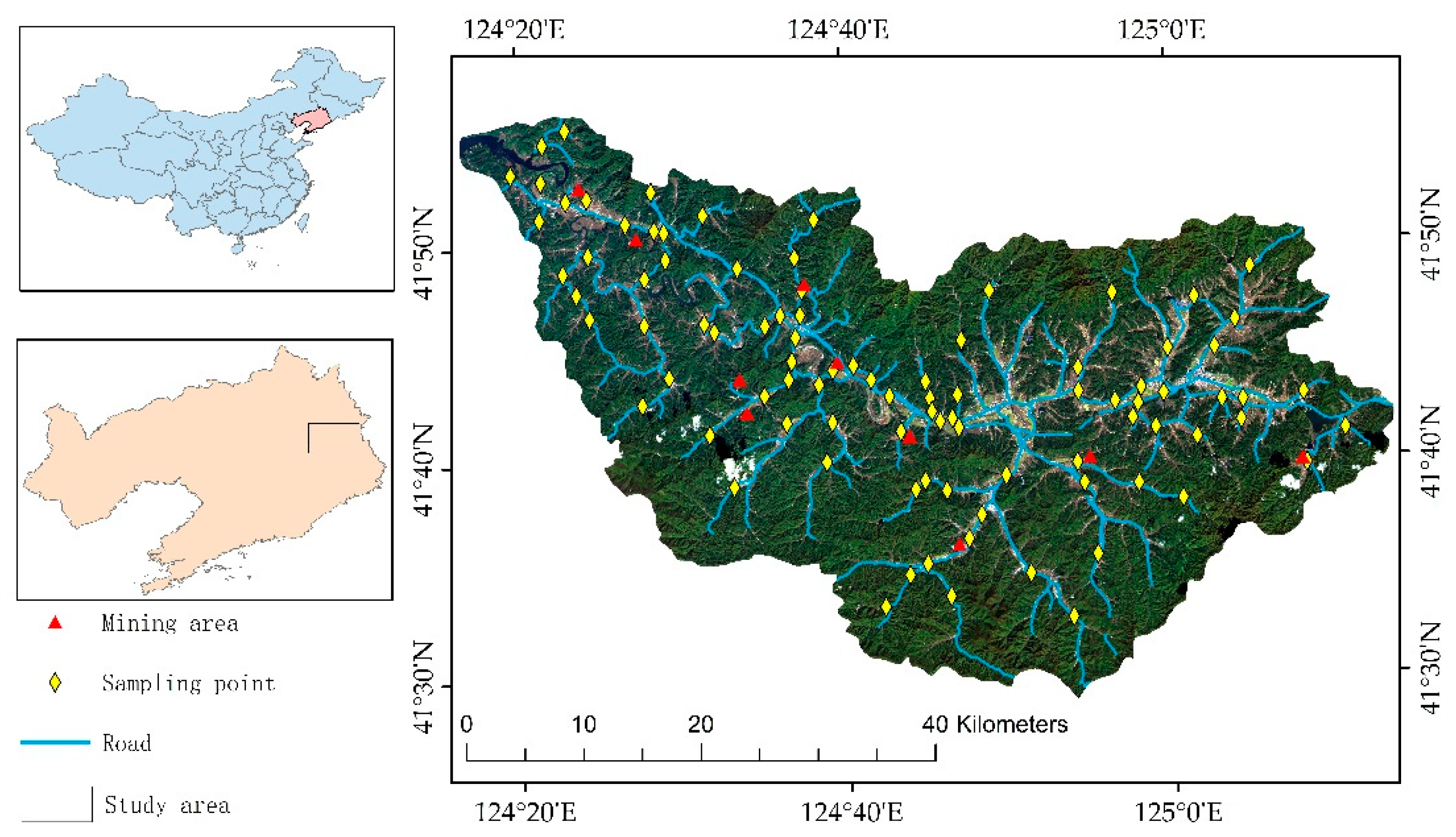
The Suzi River Basin is the main area upstream of the Dahuofang reservoir, which supplies water to cities in Liaoning Province and is rich in mineral resources. During the mining process, heavy metal(loid)s are gradually deposited into the soil, which leads to heavy metal(loid) pollution of farmland soil. Among the common heavy metal(loid)s that pollute soil, Ni, Hg, Cr, Cu, and As were used as examples in this study. Based on simple spectral indices (addition, subtraction, and ratio), advanced spectral indices (normalized difference indices) were introduced, which were used as independent variables of the model. MLR, PLSR, RFR, and ANFIS were used for modeling, and the relationship between the optimal spectral indices and the heavy metal(loid) contents in soil was discussed, thus providing a scientific and effective basis for the selection of a method of estimating heavy metal(loid) contents in soils, and providing a basis for water source protection in this area.

2. Materials and Methods

2.1. Study Area

The Suzi River is located between 124°20′00″ and 125°16′00″ E and 41°56′00″ and 41°32′00″ N (Figure 1). It is one of the first-class sub-basins in the upper reaches of the Dahuofang Reservoir and the largest river in the Xinbin Manchu Autonomous County. The Suzi River originates from the watershed in Xinbin Manchu Autonomous County. The main river course is 119 km, and the annual average runoff is 519 million m³. The soil in the study is mainly brown soil, dark brown soil, peat soil, paddy soil, white clay soil, and swamp soil area, accounting for 85% of the total land area, with an average soil thickness of 20–40 cm.

The study area is mainly mountainous, with a large area of cultivated land around the river, and industrial parks such as mining factories in some areas. At present, 11 kinds of minerals are developed in the Suzi River Basin, with iron ore and gold ore being the main ones. In the process of metal smelting, a large amount of acid mine drainage is discharged, which contains pollutants such as Ni, Hg, Cr, Cu, and As [30,31]. The effluent, having high heavy metal(loid) contents, enters the Suzi River and then the Dahuofang reservoir through the Suzi River, which could have serious environmental and ecological impacts on the water, farmland, and plants in these regions [32,33].

2.2. Data Acquisition

2.2.1. Soil Sample Collection and Chemical Analysis

The field surveys were carried out from late October until early November 2020. A total of 92 farmland surface soil samples were collected, the depth of each soil sampling point was 20 cm, and the sampling information was recorded. The soil sample was placed in a well-ventilated, lightproof place and then naturally air-dried. After the samples were passed through a uniform 100 mesh nylon net, 300 g of each sample was taken. Half of the physical soil sample (150 g) was used for chemical analyses and the other half (150 g) for spectral measurements. According to the National Environmental Protection Standards of the People’s Republic of China (HJ 781–2016, 2016) [34], Ni, Cr, and Cu contents were determined in 92 samples via inductively coupled plasma mass spectrometry (ICP-MS). According to the national standard of the People’s Republic of China (GB/T 22105.1–2008, 2008) [35], the contents of Hg and As in 92 soil samples were determined by atomic fluorescence spectrometry.

2.2.2. Spectral Pre-Treatment and Transformations

In this study, soil spectral reflectance was measured using an ASD FieldSpec^®3 portable spectrometer (Analytical Spectral Device, Boulder, CO, USA). All the soil samples were placed in wide circular containers 10 cm in diameter and 2 cm in depth. The instrument was preheated for 30 min before the measurement began. To ensure accuracy, each reflection measurement was calibrated using a standard plate with 100% reflectivity [36]. The information obtained ranged from 350 to 2500 nm, and the light source was a built-in halogen lamp, the field angle of the probe was 25°, and the sampling intervals were 1.4 nm (350–1000 nm) and 2.0 nm (1000–2500 nm). When measuring the spectrum of a soil sample, the probe was placed in contact with the surface of the soil sample. From each soil sample, we collected 10 spectral lines, and the average value of 10 spectral lines was taken as the final reflectance (Figure 2). The average spectral reflectance was calculated by ViewSpecPro V5.6 software. Due to instrument noise, spectral bands 350–399 nm and 2451–2500 nm were removed from the initial reflectivity spectra of the soil samples to improve the signal-to-noise ratio (SNR) [37].

The spectral data acquisition process is affected by the sample, instrument, experimental environment, and other factors, which may weaken the spectral signal [21]. To reduce noise interference, enhance the differences, and highlight the spectral characteristics, it is necessary to smooth and mathematically change the spectral data [12]. The breakpoints of the spectrum were removed at approximately 1000 and 1900 nm using ViewSpecPro V5.6. The Savitzky–Golay smoothing method (SG smoothing) of the second-order polynomial fitting is usually used for spectral smoothing; with a window size of 13 points, this method can effectively reduce the influence of random noise on the robustness of calibration models [38]. The SG-smoothed spectrum was taken as the original spectrum (OR), then the SG-smoothed data were transformed by seven mathematical methods, i.e., the continuum removal (CR), reciprocal (1/R), first-order differential (FDR), second-order differential (SDR), and root mean square ($\sqrt{\mathrm{R}}$). All of the transformations were implemented using MATLAB (version 2018a) software and ENVI (version 5.3).

2.3. Calculation of Optimal Spectral Indices

One of the most effective methods to analyze significant relationships between soil heavy metal(loid) contents and spectral data involves using spectral indices as the independent variables of the model, which effectively reduces the number of redundant messages and avoids dimensionality disaster [14,39]. In the calculation of spectral indices, based on the spectral reflectance after SG smoothing, all combinations were calculated in the wavelength range of 400–2450 nm, and the correlation coefficients with the soil Ni, Hg, Cr, Cu, and As contents were obtained. The combination with the largest absolute correlation coefficient was selected as the best of the corresponding spectral indices. In this study, the spectral indices mainly included the difference index (DI), ratio index (RI), the difference between the inverse reflectance of two bands (DIV), sum index (SI), and simple normalized difference spectral indices (NDSI and NPDI) [14,40]. The spectral indices are defined as:

$$\mathrm{RI}\left(R_i,R_j\right)=\raisebox{1ex}{$R_i$}\!\left/ \!\raisebox{-1ex}{$R_j$}\right.,$$

(1)

$$\mathrm{SI}\left(R_i,R_j\right)=R_i+R_j,$$

(2)

$$\mathrm{DI}\left(R_i,R_j\right)=R_i-R_j,$$

(3)

$$\mathrm{DIV}\left(R_i,R_j\right)=\raisebox{1ex}{$1$}\!\left/ \!\raisebox{-1ex}{$R_i$}\right.-\raisebox{1ex}{$1$}\!\left/ \!\raisebox{-1ex}{$R_j$}\right.,$$

(4)

$$\mathrm{NPDI}\left(R_i,R_j\right)=\left(R_i+R_j\right)\times R_j,$$

(5)

$$\mathrm{NDSI}\left(R_i,R_j\right)=\raisebox{1ex}{$\left(R_i-R_j\right)$}\!\left/ \!\raisebox{-1ex}{$\left(R_i+R_j\right)$}\right.,$$

(6)

where R is the SG-smoothing spectral reflectance value and the subscripts i and j are wavelengths in nanometers (nm).

2.4. Pearson Correlation Analysis

In order to analyze the relationship between the different soil spectral data pre-processing techniques and Ni, Hg, Cr, Cu, and As contents, the correlations between Ni, Hg, Cr, Cu, and As contents in agricultural soils and spectral indices were determined. In this study, the Pearson correlation coefficient (r) was used to determine the linear correlation between spectral reflectance and Ni, Hg, Cr, Cu, and As contents. The correlation coefficient was calculated as follows:

$$r=\frac{{\sigma }_{xy}^2}{{\sigma }_x{\sigma }_y}=\frac{\sum \left[\left(X_i-X\right)\left(Y_i-Y\right)\right]}{\sqrt{\sum {\left(X_i-X\right)}^2}\sqrt{\sum {\left(Y_i-Y\right)}^2}},$$

(7)

where r is the correlation coefficient; X is the reflectance of the corresponding band; Y is the Ni, Hg, Cr, Cu, and As content in agricultural soils; and ${\sigma }_{xy}^2$is the covariance of X and Y.

2.5. Modeling Approaches

2.5.1. Multiple Linear Regression (MLR)

MLR is a statistical model with a simple structure and is easy to calculate and interpret. It is one of the most commonly used estimation models in the field of soil science [41,42]. Like other regression techniques, it attempts to establish a relationship model between two or more independent variables and response variables by fitting a linear equation to the observed data. In this study, different spectral indices were taken as independent variables and Ni, Hg, Cr, Cu, and As contents in the soil as dependent variables to establish an MLR model. Generally, the relationship between the dependent and the independent variables is given as [43]:

$$Y=a+{\displaystyle \sum }_{i=1}^n{b}_i{x}_i+\epsilon =b_1{x}_1+b_2{x}_2+\cdots +b_i{x}_i+\epsilon ,$$

(8)

where Y is the response variable; $x_i$ (i = 1, 2, 3, …, n) are predictor variables; a is the intercept, $b_i$ (i = 1, 2, 3, …, n) is the regression coefficient; and ε is the regression residual.

2.5.2. Partial Least-Squares Regression (PLSR)

PLSR is a multivariate data analysis method. Compared with the traditional multivariate regression method, PLSR integrates the characteristics of principal component analysis, canonical correlation analysis, and multivariate linear regression analysis, which is more conducive to the identification of spectral information and noise [44,45]. Therefore, the PLSR model is widely used in the field of spectral inversion [46,47]. In this study, the PLSR model was established by Python. In the PLSR model, the spectral reflectance values under different spectral index processing methods were taken as the independent variable and the Ni, Hg, Cr, Cu, and As contents in agricultural soil were the dependent variables.

The modeling principle is as follows: establish an m × n spectrum matrix X and n × l heavy metal(loid) content detection matrix Y, where m is the spectral band number, n is the number of samples, and l is the number of different spectral indices of metal(loid)s in the soil of the same heavy metal(loid)s. X and Y can be decomposed as follows [37]:

$$\mathrm{X}=T{P}^T+E, and$$

(9)

$$\mathrm{Y}=U{Q}^T+F,$$

(10)

where U and T are the score matrixes, P and Q are the loads, and E and F are residual matrixes in the PLSR simulation. The linear regression of U and T, B is the correlation coefficient matrix, $U=TB$. The prediction formula can then be expressed by:

$$Y_{prediction}=T_{calculation}BQ=X_{measure}{P}^{T}BQ,$$

(11)

2.5.3. Random Forest Regression (RFR)

RFR is a predictive modeling algorithm based on the regression tree (CART) and bagging learning strategy first developed by Breiman [37]. In the process of model training, a certain number of bootstrap samples were extracted from the original data set to train each tree, and randomly selected features were split for each decision [48]. Due to the introduction of randomness, over-fitting does not easily occur in RFR. The RFR model has the advantages of high prediction accuracy, good performance on unbalanced data sets, and robustness to noise [37,49]. In this study, an RFR model was developed in Python software using the RFR software package, and 100 trees were used to train the RFR model by correlating Ni, Hg, Cr, Cu, and As contents with spectral indices. When the smallest sample in the tree was a sample with zero impurity, the model training was stopped. The trained forest ${\widehat{F}}_{RF}^K\left(x\right)$ with K trees can be expressed as [50]:

$${\widehat{F}}_{RF}^K\left(x\right)=\frac{1}{K}{{\displaystyle \sum }}_{K=1}^{K}T\left(x_s\right),$$

(12)

where T(x) is a single tree, x is all the training samples, and $x_s$ is each tree’s training sample data obtained with the bootstrap sampling method. Another parameter that is not noted in Equation (12) is the number of subattributes selected from all the attributes with bootstrap sampling.

2.5.4. Adaptive Neuro-Fuzzy Inference System (ANFIS)

The adaptive neuro-fuzzy reasoning system (ANFIS) is a computational intelligence modeling method that combines the learning ability of neural networks with the reasoning ability of fuzzy logic and is often used to model computational nonlinear complex problems [51,52]. The structure of ANFIS includes an antecedent part and a conclusion part, which are connected by fuzzy rules in the form of a network [53]. In this study, the ANFIS algorithm embedded in the fuzzy reasoning toolbox of MATLAB was used to build the model. The coverage threshold was fixed at 0.05 and the training stopped when the error stabilized.

The ANFIS has five layers; the output of the first layer is shown in Equation (13):

$$Q_{1,i}={\mu }_{A_i}\left(x\right),$$

(13)

where ${\mu }_A$ is a membership function, x is the input of node i, and $Q_{1,i}$ is a membership value. The output of the second layer is an algebraic product of the input signals, as shown in Equation (14):

$$Q_{2,i}={\omega }_i={\mu }_{A_i}\left(x_1\right)\times \cdots \times {\mu }_{C_i}\left(x_n\right),$$

(14)

In the third layer, the ratio of the ith rule’s firing strength to the total summation of all rules’ firing strength is calculated in each node, as shown in Equation (15):

$$Q_{3,i}=\overline{{\omega }_i}=\frac{{\omega }_i}{{\omega }_1+\cdots +{\omega }_n},$$

(15)

In the fourth layer, the output of each node is as shown in Equation (16):

$$Q_{4,i}=\sum \overline{{\omega }_i}{f}_i,$$

(16)

where $f_i$ is the corresponding function of each node. The overall output is computed in the fifth layer using Equation (17):

$$Q_{5,i}=\frac{{{\displaystyle \sum }}_{i=1}^n{\omega }_i{f}_i}{{{\displaystyle \sum }}_{i=1}^n{\omega }_i},$$

(17)

2.6. Model Validation

In this study, the samples were arranged in ascending order according to the contents of the heavy metal(loid)s in the soil, and each metal(loid) element was divided into a training set and verification set in a ratio of 3:1. The training set contained 69 samples and the validation set contained 23 samples. These models were established by taking the optimized spectral indices as the independent variables and Ni, Hg, Cr, Cu, and As content as the dependent variables, and the determination coefficient (${\mathrm{R}}^2$), root mean square error (RMSE), and residual predictive deviation (RPD) were selected as accuracy indices to measure the predictability of the model. The calculation formulae of ${\mathrm{R}}^2$, RMSE, and MAE are as follows, respectively:

$${\mathrm{R}}^2=1-\frac{{{\displaystyle \sum }}_{i=1}^n{\left(\widehat{y_i}-y_i\right)}^2}{{{\displaystyle \sum }}_{i=1}^n{\left(y_i-\overline{y}\right)}^2},$$

(18)

$$\mathrm{RMSE}=\sqrt{\frac{{{\displaystyle \sum }}_{i=1}^n{\left(y_i-{\widehat{y}}_i\right)}^2}{n}},$$

(19)

$$\mathrm{RPD}=\frac{\sigma }{\sqrt{{{\displaystyle \sum }}_{i=1}^n{\left(y_i-\widehat{y_i}\right)}^2/n}},$$

(20)

where $y_i$ is the measured Ni, Hg, Cr, Cu, and As content in the soil; $\widehat{y_i}$ is the estimated soil Ni, Hg, Cr, Cu, and As content; $\overline{y}$is the mean of the measured soil Ni, Hg, Cr, Cu, and As content; and n is the number of soil samples, σ is the standard deviation of the measured reference values.

3. Results

3.1. Descriptive Statistics of Ni, Hg, Cr, Cu, and As Contents in Agricultural Soil

The statistical characteristics of the Ni, Hg, Cr, Cu, and As contents in the study area are shown in

Table 1. Descriptive statistics of Ni, Hg, Cr, Cu, and As contents in agricultural soil.

Element	Number	Min (mg/kg)	Max (mg/kg)	Mean (mg/kg)	SD (mg/kg)	CV (%)	Skew-Ness	Kurtosis
Ni	92	14.900	56.040	31.740	8.425	26.544	0.668	0.402
Hg	92	0.008	0.591	0.092	0.086	93.478	3.059	12.539
Cr	92	0.890	181.200	76.658	3.489	4.551	−0.033	0.349
Cu	92	3.600	133.400	40.346	15.216	37.714	2.550	14.969
As	92	3.680	21.680	8.682	3.684	42.433	1.463	2.160

SD: standard deviation; CV: coefficient of variation.

. Compared with the risk control standard for soil contamination of agricultural land (GB 15618–2018), the contents of Ni, Hg, and As in agricultural soils were lower than the screening value of soil pollution risk in agricultural land (70.00, 1.80, and 40.00 mg/kg, respectively), and some Cr and Cu values were higher than the screening value of soil pollution risk (150.00 and 50.00 mg/kg, respectively). We found significant differences in the minimum and maximum values of Ni, Hg, Cr, Cu, and As contents in agricultural soil. The standard deviation, skewness, and kurtosis of Ni, Cr, and As are small, whereas those of Hg and Cu are large, indicating that certain differences exist in the contents of Ni, Cr, and As in the agricultural soil in different regions in the study area, with significant differences in Hg and Cu. The coefficient of variation (CV) is an important index reflecting the fluctuation in environmental variables: the CV of Cr is smaller than that of Ni, Hg, Cu, and As, which reflects that human activities have a stronger influence on the contents of Ni, Hg, Cu, and As than on Cr in agricultural soil [54]. In total, the contents of copper and chromium are high, indicating they are seriously polluting the agricultural soil. Although the contents of Ni, Hg, and As did not reach pollution levels, some soil samples had high levels. Through proximity analysis (Figure 1 and

Table 2. Descriptive statistics of sampling point distance from mine and road.

	Number	Min (km)	Max (km)	Mean (km)	SD (km)
Mining area	92	0.531	16.944	5.468	3.389
Road	92	0.005	1.323	0.165	0.214

), we found that the samples with high heavy metal(loid) contents were all obtained near mining areas and roads, indicating that the agricultural soil in this area is severely polluted by heavy metal(loid)s due to the processes of mineral mining and transportation. In this study, through the correlation analysis of Ni, Hg, Cr, Cu, and As contents, we found that except for the general correlation between Ni and Cr, the Poisson coefficient is 0.642, and no correlation was found between other heavy metal(loid) elements. Therefore, it was feasible for estimating Ni, Hg, Cr, Cu, and As content in agriculture soils.

3.2. Soil Spectral Characteristics Analysis

Figure 2 shows the original reflectance spectra (Figure 2A) and the reflectance spectra after SG smoothing (Figure 2B) of the soil samples in the Suzi River Basin. The spectral reflectance values of all the soil samples showed certain differences, but with an increasing trend, and the spectral reflectance ranged from 0.05 to 0.8. The spectral differences among soil samples were mainly caused by the different contents of each component, which led to certain differences in spectral reflectance of the soil samples. In the range of 500–800 nm, the reflectivity value increased rapidly, and the slope of the spectral curve was large, so the spectral absorption peak could not be seen. From 800 to 2300 nm, the spectral reflectance tended to rise steadily, with obvious spectral absorption peaks at 1000, 1415, 1910, and 2200 nm. In the range of 500–800 nm, the spectral curves showed a downward trend. In this study, to highlight the spectral characteristics of the band, SG-smoothing spectral reflectance data as the original spectral reflectance (OR), and five spectrum transform methods (CR, 1/R, FDR, SDR, and $\sqrt{\mathrm{R}}$) were established to conduct parallel background value separation (Figure 3). These methods effectively extracted the spectral information that was not easy to identify in the original band, and the position of the spectral characteristic band was more obvious. The reflectivity changed rapidly in the range of 400–593 nm, and we observed two weak absorption peaks near 430 and 490 nm. In the range of 594–1374 nm, the slope of the soil spectral curve decreased, and the weak reflection peak appeared near 590 and 810 nm. We observed several characteristic absorption bands and reflection peaks in the spectral curve from 1375 to 2450 nm, with an obvious adsorption valley near 1415 nm. The spectral curve showed a V-shape from 1856 to 2129 nm. A visible absorption valley was observed near 1910 nm. The spectral curves fluctuated from 2129 to 2450 nm, and two absorption valleys appeared near 2200 and 2327 nm.

3.3. Correlation Analysis between Soil Spectrum and Ni, Hg, Cr, Cu, and As Contents

By calculating the correlation between the contents of Ni, Hg, Cr, Cu, and As in the agricultural soil samples and the transformation spectrum, the correlation coefficient curve between the soil spectral variables and the contents of Ni, Hg, Cr, Cu, and As was obtained (Figure 4). Compared with the original spectrum (OR), the correlation coefficient curves of different transformed spectra are significantly different. The correlation coefficient curves of 1/R and √R are relatively smooth, and the absolute value of the maximum correlation coefficient is less than 0.2. Among them, are the positive and negative correlation between Ni and Cu contents and the spectra transformed at about 1200 nm; Hg and As contents are positively correlated with the spectral curves after $\sqrt{\mathrm{R}}$ transformation, but negatively correlated with the spectral curves after 1/R transformation; the correlation between Cr content and the spectral curve after 1/R transformation changed at 1600 and 1900 nm, and negatively correlated with the spectral curve after $\sqrt{\mathrm{R}}$ transformation. After CR, FDR, and SDR transformation, the spectral correlation coefficients of the three heavy metals fluctuated between positive and negative within the Vis–NIR range. The correlation coefficient significantly increased compared with the original spectral correlation. Compared with the visible spectrum (400–700 nm), the near-infrared spectrum (700–2500 nm) curve has a more obvious range, which indicates that their spectral response is more obvious in the near-infrared spectrum. The maximum correlation coefficients between the contents of Ni, Hg, Cr, Cu, and As in agricultural soil and the spectra are shown in

Table 3. The maximum absolute value of the correlation coefficient between Ni, Hg, Cr, Cu, and As contents and spectra.

Maximum Correlation	OR	CR	1/R	FDR	SDR	$\sqrt{{R}}$
Ni	0.145	0.617	0.148	0.670	0.445	0.147
Hg	0.123	0.231	0.151	0.229	0.283	0.131
Cr	0.201	0.540	0.177	0.495	0.385	0.198
Cu	0.104	0.330	0.093	0.328	0.348	0.102
As	0.305	0.422	0.295	0.434	0.448	0.131

; the correlation coefficient between the OR and soil Ni, Hg, and Cr contents is low. After the 1/R and $\sqrt{\mathrm{R}} \mathrm{transformation}$, the spectral correlation slightly increased, by about 0.003, but the correlation between the transformed spectra and As and Cu contents reduced. However, after CR, FDR, and SDR transformation, the correlation between the spectrum and the soil Ni, Hg, Cr, Cu, and As contents significantly increased compared with the original spectrum. Among them, the correlation between FDR spectra and Ni content significantly improved by about 0.5, and the correlation of other elements also significantly improved by at least 0.1. Therefore, the findings show that although spectral transformation can highlight hidden spectral information, it is not feasible to directly estimate heavy metal(loid) content in agricultural soils using spectral data.

3.4. Correlation between Optimal Spectral Indices and Ni, Hg, Cr, Cu, and As Contents

In order to reduce the redundancy information in the spectrum using the optimal band combination algorithm, the correlation coefficient between soil heavy metal(loid) content and spectral indices was used. The spectral indices optimized by different spectral conversion methods and the correlation coefficient are shown in

Table 4. The bands and correlation coefficients of optimal spectral indices for Ni.

Transform Method	Optimal Spectral Indices	Correlation Coefficient 1
OR	DIV2272,2271, NPDI408,408, RI2268,2269, DI2269,2271, NDSI2268,2269, SI408,408	0.613, 0.138, 0.701, 0.671, 0.701, 0.145
CR	DIV2271,2269, NPDI2344,2256, RI2088,2272, DI2269,2271, NDSI2269,2271, SI2257,2358	0.709, 0.653, 0.711, 0.712, 0.710, 0.648
1/R	DIV2269,2271, NPDI403,403, RI2269,2268, DI2272,2271, NDSI2269,2268, SI405,405	0.671, 0.143, 0.701, 0.613, 0.701, 0.148
FDR	DIV2265,753, NPDI2268,2384, RI2269,735, DI2102,2268, NDSI734,2268, SI1732,2270	0.665, 0.636, 0.718, 0.704, 0.729, 0.714
SDR	DIV1031,1485, NPDI2298,2293, RI1392,1918, DI2294,2267, NDSI2308,2294, SI2288,2295	0.496, 0.605, 0.538, 0.620, 0.527, 0.650
$\sqrt{\mathrm{R}}$	DIV2271,2268, NPDI408,408, RI2268,2269, DI2268,2269, NDSI2268,2269, SI406,406	0.661, 0.145, 0.701, 0.702, 0.701, 0.147

¹ Correlation coefficient is the largest absolute value of the correlation coefficient.

,

Table 5. The bands and correlation coefficients of optimal spectral indices for Hg.

Transform Method	Optimal Spectral Indices	Correlation Coefficient 1
OR	DIV2073,2071, NPDI407,2450, RI2065,2086, DI1762,1761, NDSI2065,2086, SI407,1915	0.285, 0.109, 0.273, 0.229, 0.273, 0.127
CR	DIV455,456, NPDI1888,2315, RI456,455, DI456,455, NDSI456,455, SI1038,1427	0.370, 0.264, 0.377, 0.380, 0.377, 0.268
1/R	DIV1762,1761, NPDI1915,1915, RI2086,2065, DI2073,2071, NDSI2086,2065, SI1915,1915	0.229, 0.162, 0.273, 0.285, 0.273, 0.151
FDR	DIV1302,1734, NPDI2291,1762, RI1736,1308, DI1760,1804, NDSI2314,606, SI468,1373	0.671, 0.362, 0.661, 0.336, 0.678, 0.327
SDR	DIV1628,1184, NPDI1042,615, RI700,1629, DI554,1767, NDSI2246,2413, SI680,1767	0.683, 0.558, 0.680, 0.405, 0.697, 0.383
$\sqrt{\mathrm{R}}$	DIV2078,2068, NPDI407,1516, RI2065,2086, DI1762,1761, NDSI2065,2086, SI407,1915	0.293, 0.123, 0.273, 0.199, 0.273, 0.136

¹ Correlation coefficient is the largest absolute value of the correlation coefficient.

,

Table 6. The bands and correlation coefficients of optimal spectral indices for Cr.

Transform Method	Optimal Spectral Indices	Correlation Coefficient 1
OR	DIV2252,2233, NPDI761,761, RI2275,2229, DI2232,2252, NDSI2229,2266, SI756,756	0.511, 0.202, 0.562, 0.501, 0.561, 0.201
CR	DIV2236,2275, NPDI2232,2443, RI2236,2275, DI2236,2275, NDSI2236,2275, SI2229,2443	0.552, 0.576, 0.552, 0.552, 0.552, 0.554
1/R	DIV2232,2252, NPDI930,955, RI2229,2266, DI2252,2233, NDSI2266,2229, SI767,929	0.501, 0.167, 0.561, 0.511, 0.561, 0.177
FDR	DIV2232,1622, NPDI2146,2251, RI1170,2424, DI1100,2251, NDSI2336,2238, SI1770,2240	0.481, 0.597, 0.576, 0.568, 0.535, 0.562
SDR	DIV735,745, NPDI2241,1122, RI2191,2348, DI1397,2021, NDSI1921,1902, SI1012,1394	0.481, 0.553, 0.496, 0.528, 0.498, 0.529
$\sqrt{\mathrm{R}}$	DIV2251,2250, NPDI756,756, RI2266,2229, DI2232,2270, NDSI2229,2266, SI756,751	0.547, 0.201, 0.561, 0.545, 0.561, 0.198

¹ Correlation coefficient is the largest absolute value of the correlation coefficient.

,

Table 7. The bands and correlation coefficients of optimal spectral indices for Cu.

Transform Method	Optimal Spectral Indices	Correlation Coefficient 1
OR	DIV2237,2137, NPDI670,670, RI2266,2252, DI2268,2269, NDSI2252,2266, SI670,670	0.336, 0.107, 0.394, 0.335, 0.394, 0.104
CR	DIV2271,2252, NPDI2225,2315, RI2252,2272, DI2252,2272, NDSI2252,2272, SI2224,2325	0.422, 0.390, 0.423, 0.424, 0.423, 0.396
1/R	DIV2268,2269, NPDI711,705, RI2252,2266, DI2237,2227, NDSI2266,2252, SI685,685	0.335, 0.087, 0.394, 0.336, 0.394, 0.093
FDR	DIV2132,1834, NPDI2248,2229, RI2270,1834, DI1150,2229, NDSI468,2191, SI2148,2228	0.668, 0.396, 0.664, 0.416, 0.723, 0.416
SDR	DIV1192,1479, NPDI911,1066, RI1147,1479, DI1217,825, NDSI911,2214, SI634,828	0.726, 0.618, 0.716, 0.436, 0.732, 0.428
$\sqrt{\mathrm{R}}$	DIV2264,2251, NPDI670,670, RI2252,2266, DI2261,2263, NDSI2252,2266, SI670,670	0.371, 0.104, 0.394, 0.375, 0.374, 0.102

¹ Correlation coefficient is the largest absolute value of the correlation coefficient.

and

Table 8. The bands and correlation coefficients of optimal spectral indices for As.

Transform Method	Optimal Spectral Indices	Correlation Coefficient 1
OR	DIV1314,1141, NPDI954,954, RI2330,2346, DI2331,2334, NDSI2229,2266, SI2330,2346	0.440, 0.305, 0.445, 0.437, 0.445, 0.305
CR	DIV2379,2396, NPDI2376,2418, RI2396,2379, DI2396,2379, NDSI2396,2379, SI2376,2419	0.572, 0.533, 0.573, 0.572, 0.573, 0.522
1/R	DIV2331,2334, NPDI988,988, RI2346,2330, DI1413,1411, NDSI2346,2330, SI975,975	0.437, 0.285, 0.445, 0.440, 0.445, 0.295
FDR	DIV1404,2264, NPDI2022,2415, RI2414,1535, DI2388,2414, NDSI2030,2332, SI1477,2414	0.413, 0.567, 0.603, 0.623, 0.569, 0.589
SDR	DIV1941,1736, NPDI470,2354, RI1041,765, DI1451,1397, NDSI634,2182, SI1397,1548	0.525, 0.552, 0.584, 0.514, 0.563, 0.554
$\sqrt{\mathrm{R}}$	DIV2251,2250, NPDI756,756, RI2266,2229, DI2232,2270, NDSI2229,2266, SI756,751	0.445, 0.305, 0.445, 0.439, 0.445, 0.304

¹ Correlation coefficient is the largest absolute value of the correlation coefficient.

. The correlation patterns between different spectral conversion methods are different. According to a comparative analysis with Table 3, except for a few spectral indices, the correlation between them and soil heavy metal(loid) contents decreased: most of the spectral indices were higher than the single-band spectral correlation. The index of reduced spectral correlation is NPDI, and it mainly occurred in the spectrum transformed by the original spectrum and $\sqrt{\mathrm{R}}$; however, after CR, FDR, and SDR transform, the correlation with NPDI significantly improved compared with single bands. For other indices (DIV, RI, DI, NDSI, and SI), regardless of the original spectrum or the spectrum after mathematical transformation (CR, 1/R, FDR, SDR, and $\sqrt{\mathrm{R}}$), their correlation coefficients with soil heavy metal(loid) contents were higher than their correlation coefficients with a single band. To summarize, the correlation between the optimal spectral indices and the contents of Ni, Hg, Cr, Cu, and As in agricultural soils was significantly higher than that of the optimal single band, which indicated that it is feasible to use spectral indices to study the contents of Ni, Hg, Cr, Cu, and As in agricultural soils.

3.5. The Establishment and Verification of the Spectral Prediction Model

In this study, these optimized spectral indices were selected as independent variables and soil Ni, Hg, Cr, Cu, and As contents as dependent variables. MLR, PLSR, RFR, and ANFIS were used to analyze the relationship between spectral data and soil Ni, Hg, Cr, Cu, and As contents. The significance test was conducted at the 0.01 level, and the accuracy of the model results is shown in

Table 9. The estimation models of Ni content and their evaluation indices.

Transform Method	MLR			PLSR			RFR			ANFIS
	R2	RMSE	RPD	R2	RMSE	RPD	R2	RMSE	RPD	R2	RMSE	RPD
OR	0.585	6.077	1.586	0.506	6.634	1.453	0.498	6.685	1.442	0.284	7.094	1.208
CR	0.595	6.005	1.605	0.522	6.524	1.478	0.502	6.658	1.448	0.315	6.936	1.236
1/R	0.583	6.094	1.582	0.515	6.574	1.467	0.483	6.786	1.421	0.302	7.005	1.223
FDR	0.676	5.373	1.794	0.651	5.576	1.729	0.510	6.605	1.460	0.373	6.636	1.292
SDR	0.713	5.053	1.908	0.595	6.003	1.606	0.201	8.434	1.143	- 1	- 1	- 1
$\sqrt{\mathrm{R}}$	0.601	5.963	1.617	0.525	6.503	1.483	0.563	6.238	1.546	0.334	6.839	1.253

¹ Model prediction failure.

,

Table 10. The estimation models of Hg content and their evaluation indices.

Transform Method	MLR			PLSR			RFR			ANFIS
	R2	RMSE	RPD	R2	RMSE	RPD	R2	RMSE	RPD	R2	RMSE	RPD
OR	0.050	0.123	1.048	0.031	0.124	1.038	0.010	0.125	1.027	- 1	- 1	- 1
CR	0.084	0.121	1.068	0.080	0.121	1.065	0.214	0.112	1.152	0.235	0.079	1.151
1/R	0.005	0.126	1.024	0.019	0.125	1.031	0.059	0.130	1.012	- 1	- 1	- 1
FDR	0.013	0.125	1.028	0.507	0.088	1.455	0.083	0.121	1.067	0.280	0.060	1.205
SDR	0.638	0.076	1.697	0.653	0.074	1.733	0.519	0.087	1.473	0.282	0.060	1.206
$\sqrt{\mathrm{R}}$	0.073	0.121	1.061	0.042	0.123	1.044	0.154	0.115	1.111	- 1	- 1	- 1

¹ Model prediction failure.

,

Table 11. The estimation models of Cr content and their evaluation indices.

Transform Method	MLR			PLSR			RFR			ANFIS
	R2	RMSE	RPD	R2	RMSE	RPD	R2	RMSE	RPD	R2	RMSE	RPD
OR	0.216	33.423	1.153	0.265	32.362	1.191	0.229	33.145	1.163	- 1	- 1	- 1
CR	0.254	32.592	1.183	0.224	33.240	1.160	0.357	30.258	1.274	0.309	26.355	1.230
1/R	0.132	35.153	1.097	0.260	32.471	1.187	0.286	31.882	1.209	0.133	29.515	1.098
FDR	0.488	27.000	1.428	0.491	26.917	1.432	0.353	30.358	1.270	0.411	24.318	1.333
SDR	0.576	24.576	1.569	0.603	23.777	1.621	0.338	30.708	1.255	0.520	21.885	1.481
$\sqrt{\mathrm{R}}$	0.258	32.511	1.186	0.250	32.694	1.179	0.448	28.036	1.375	0.101	30.057	1.078

¹ Model prediction failure.

,

Table 12. The estimation models of Cu content and their evaluation indices.

Transform Method	MLR			PLSR			RFR			ANFIS
	R2	RMSE	RPD	R2	RMSE	RPD	R2	RMSE	RPD	R2	RMSE	RPD
OR	- 1	- 1	- 1	0.022	21.095	1.034	0.018	21.139	1.043	- 1	- 1	- 1
CR	0.019	21.125	1.032	0.032	20.981	1.039	- 1	- 1	- 1	- 1	- 1	- 1
1/R	- 1	- 1	- 1	0.013	21.194	0.029	0.039	20.906	1.043	- 1	- 1	- 1
FDR	0.855	8.113	2.688	0.732	11.047	1.974	0.206	19.005	1.147	0.158	11.112	1.114
SDR	0.417	16.291	0.339	0.571	13.977	1.560	0.488	15.263	1.429	- 1	- 1	- 1
$\sqrt{\mathrm{R}}$	- 1	- 1	- 1	- 1	- 1	- 1	- 1	- 1	- 1	- 1	- 1	- 1

¹ Model prediction failure.

and

Table 13. The estimation models of As content and their evaluation indices.

Transform Method	MLR			PLSR			RFR			ANFIS
	R2	RMSE	RPD	R2	RMSE	RPD	R2	RMSE	RPD	R2	RMSE	RPD
OR	0.317	3.584	1.156	0.201	3.621	1.144	0.172	3.686	1.124	- 1	- 1	- 1
CR	0.412	3.106	1.334	0.365	3.229	1.283	0.249	3.510	1.180	- 1	- 1	- 1
1/R	0.211	3.599	1.151	0.213	3.594	1.153	0.116	3.809	1.088	- 1	- 1	- 1
FDR	0.565	2.672	1.550	0.528	2.782	1.489	0.554	2.705	1.531	- 1	- 1	- 1
SDR	0.723	2.312	1.943	0.775	1.923	2.154	0.371	3.214	1.289	0.531	2.285	1.493
$\sqrt{\mathrm{R}}$	0.240	3.523	1.173	0.223	3.571	1.160	0.295	3.402	1.218

¹ Model prediction failure.

. The results of the models show that in the estimation of different heavy metal(loid)s, the performance of the four algorithms varies widely. In the Ni estimation model, the ANFIS algorithm failed to model the spectral data after SDR conversion, and no statistical data were obtained in this process. The accuracy of the MLR and PLSR models was significantly higher than that of the RFR and ANFIS models, and the PLSR model was more accurate than the MLR model, and the accuracy of the model was ${\mathrm{R}}^2=0.713$, RMSE = 5.053, and RPD = 1.908. For Hg, the ANFIS algorithm failed to model spectral data after OR, 1/R, and $\sqrt{\mathrm{R}}$ conversion. The RFR model accuracy of CR, 1/R, and $\sqrt{\mathrm{R}}$ was higher than that of MLR and PLSR, but it could not meet the modeling accuracy requirement (${\mathrm{R}}^2<0.22$). Among the FDR and SDR models, the PLSR model of SDR produced the best effect, with a model accuracy of ${\mathrm{R}}^2=0.653$, RMSE = 74.244, and RPD = 1.733. In the estimation model of Cr, the PLSR model of SDR also worked best (${\mathrm{R}}^2=0.603$, RMSE = 23.777, and RPD = 1.621), producing much higher accuracy than other models. In the As estimation model, the prediction effect of MLR and PLSR models was found to be better than that of RFR and ANFIS, and the PLSR model after SDR spectral transformation produced the best prediction effect$({\mathrm{R}}^2=0.775$, RMSE = 1.923, and RPD = 2.154). In the model for estimating Cu, compared with Ni, Hg, Cr, and As, the MLR model with FDR transformation had the best effect (${\mathrm{R}}^2=0.855$, RMSE = 8.113, and RPD = 2.688), and produced the best prediction effect among the five heavy metal(loid)s. In conclusion, in the estimation models of soil Ni, Hg, Cr, As, and Cu contents, a better model effect was produced by FDR and SDR mathematical transformation spectral indices as model independent variables than by other spectral transformations used, and the MLR and PLSR model accuracy was better than that of RFR and ANFIS, with ${\mathrm{R}}^2$ values all above 0.6 and RPD values all above 1.5. These results show that this method could accurately estimate samples and has strong predictive ability for soil Ni, Hg, Cr, Cu, and As contents [55,56].

The scatterplots of the optimal models of Ni, Hg, Cr, Cu, and As contents are shown in Figure 5. The scatterplots diagram shows that the model has a good effect on the prediction of soil Ni, Hg, Cr, Cu, and As contents. However, discrete points can be found in all of these heavy metal(loid)s. The main reason for this is that the selection of modeling and validation data sets in the modeling process, soil samples with the highest heavy metal(loid) contents will inevitably be used in the validation set. A number of mining areas are located in the study area, and mining and transportation cause heavy metal(loid) pollution in agriculture soil. In the process of soil sampling, some sampling sites were close to mining areas and transportation roads. Therefore, some soil samples had high heavy metal(loid) contents, which shows that it is vital to monitor the heavy metal(loid) contents in agriculture soil near mining areas.

The results of this study show that pre-treatment of soil spectral data is an effective method to improve the accuracy of spectral modeling. Proper pre-treatment could effectively highlight the spectral characteristic bands of soil heavy metal(loid)s and increase the prominence of the reflection peak and absorption valley of the spectral. When establishing models for estimation of Ni, Hg, Cr, Cu, and As contents, a strong linear relationship exists between the optimized spectral indices and the contents of Ni, Hg, Cr, Cu, and As in soil. Therefore, the simple MLR algorithm has a more accurate model prediction effect, and the modeling process takes advantage of the benefits of the algorithm, such as simplicity and speed. The PLSR algorithm, which organically combines the advantages of multiple linear regression, principal component analysis, and canonical correlation analysis, provides advantages that other methods cannot when solving linear problems and achieves accurate prediction results. Finally, the results also show that it is reasonable and feasible to estimate heavy metal(loid) contents in soil based on the combined optimized spectral indices method.

4. Discussion

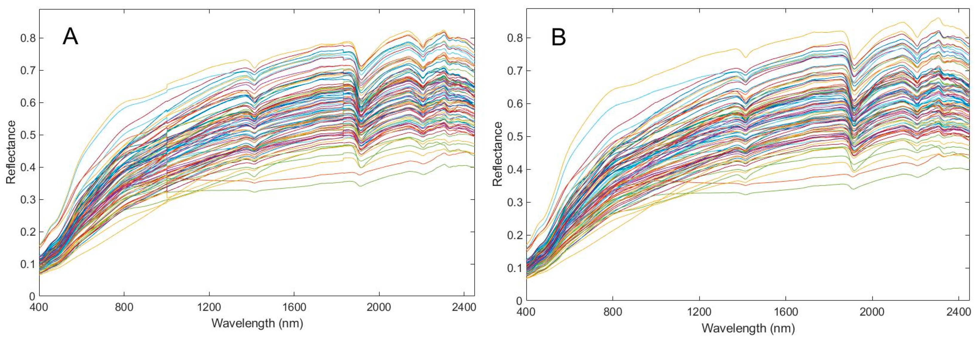
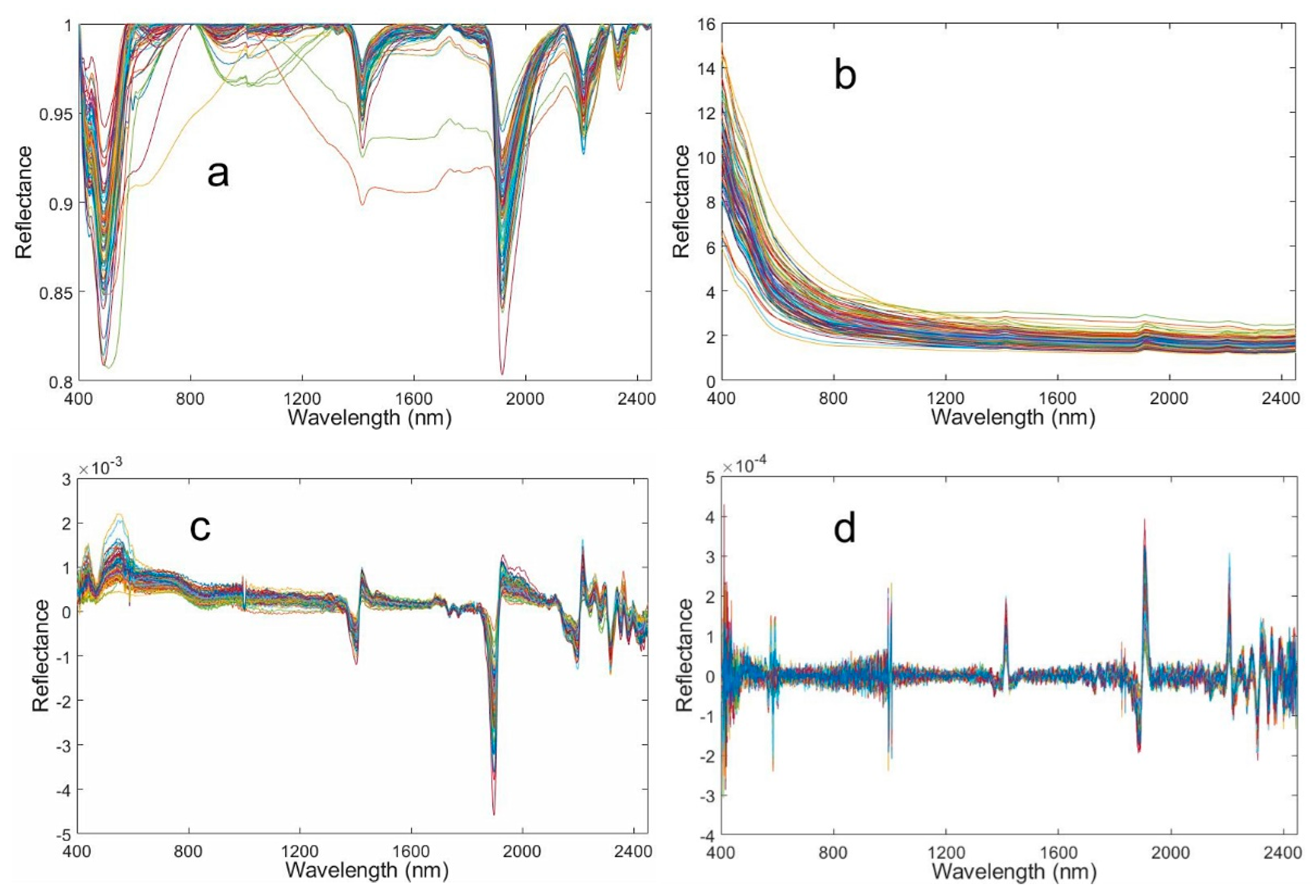
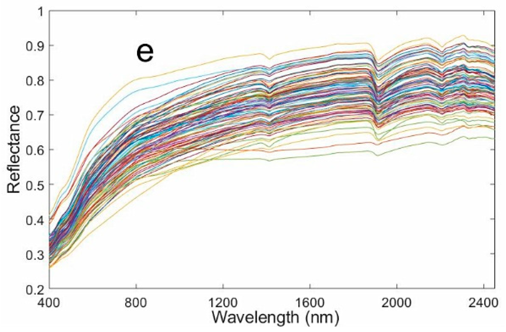
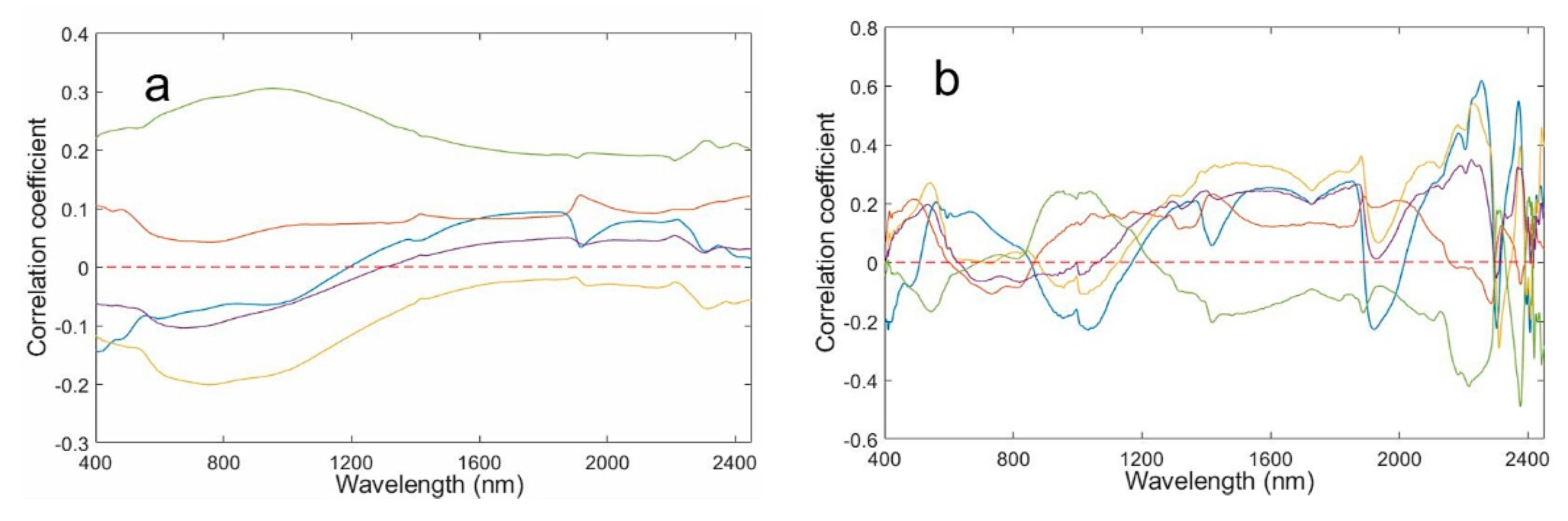
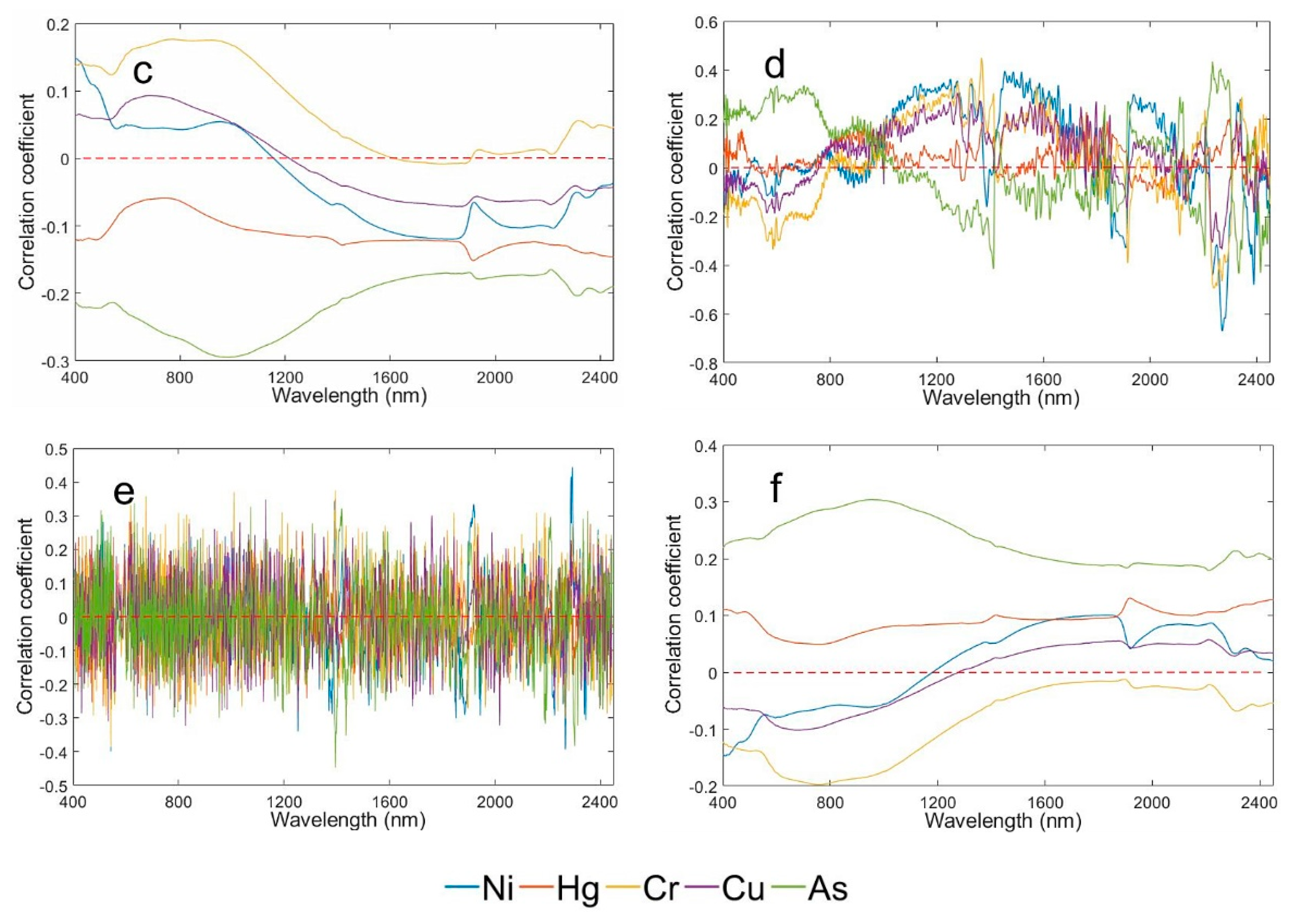
Through the analysis of the original spectrum and the mathematically transformed spectrum, we found that the spectral resolution and sensitivity of the transformed spectrum were significantly improved, and many weak absorption peaks were amplified. These transformations effectively eliminated the influence of the parallel background values and extracted the spectral information. In these mathematical transformations, the first derivative and the second derivative resulted in higher model accuracy. In this study, the accuracy of Ni and Cu estimated using the first derivative was higher than that of the second derivative model, whereas the estimation accuracy for Hg, Cr, and As was higher using the second derivative. The main reason for this finding is that the first derivative can enhance the spectral information while maintaining the continuity and integrity of the spectral information [57,58]. For the second derivative, the optimal band combination algorithm was used in this study to process the spectrum, which effectively removed the influence of additional spectral noise caused by the higher derivative. According to the spectral index calculation in Table 4, Table 5, Table 6, Table 7 and Table 8, 21 wavelengths were selected from the spectrum of the five heavy metal(loid)s, including 468, 606, 734, 825, 1100, 1170, 1192, 1184, 1217, 1477, 1535, 1628, 1732, 2146, 2191, 2251, 2268, 2314, 2388, 2414, and 2424 nm. Some studies showed that these wavelengths are close to the absorption characteristics of hematite, ferrihydrite, Fe³⁺, goethite, illite, and organic matter [17,59,60], and are strongly correlated with the spectral characteristics of N-H, C-H, O-H$, {\mathrm{CO}}_3^{2-}$ group, and -OH stretching vibration of water molecules in agricultural soil [14,61]. The main reason for this is the adsorption of heavy metal(loid)s by organic matter and iron/manganese minerals in soil, which is mainly related to the electronic transition of metal ions [62]. In addition, the chemical bond stretching, the stretching vibration of the water molecular –OH in the soil silicate minerals, and the absorption of water molecules are also main reasons [63,64,65].

Spectral transformation is a necessary and effective method for the prediction modelling of soil heavy metal(loid)s [66]. Appropriate transformation can effectively highlight the characteristic bands of the spectrum, make the reflection peak and absorption valley of the spectral curve more prominent, and enhance the correlation between the soil spectrum and heavy metal(loid) content, so as to improve the prediction accuracy of the model. SG-smoothing pre-processing can eliminate the multiplicative interference of granularity, separating and removing complex effects, and leaving accurate soil spectral information [67]. The SG-smoothed spectra were transformed by different mathematical methods, which improved the correlation between soil spectra and heavy metal(loid) content, especially the first and second derivatives. The results showed that the derivative transformation of the spectrum can distinguish similar spectra and effectively highlight the absorption characteristics of the spectrum. However, the integer derivative tends to ignore the progressive changes in the spectrum and curvature in the slit, resulting in the loss of subtle information [68]. Previous studies also showed that the combination of different spectral pre-treatment methods can improve the prediction accuracy of the model [5,11], which agrees with the findings of other studies [5,61,69].

In this study, six optimal spectral indices (DIV, NPDI, RI, DI, NDSI, and SI) were used to investigate the feasibility of using spectral indices for the prediction of soil Ni, Hg, Cr, Cu, and As contents. A correlation between six spectral indices and soil Ni, Hg, Cr, Cu, and As contents was found. Compared with the correlation of the optimal characteristic bands (Table 2), the correlation between the spectral indices and soil Ni, Hg, Cr, Cu, and As contents was significantly stronger.

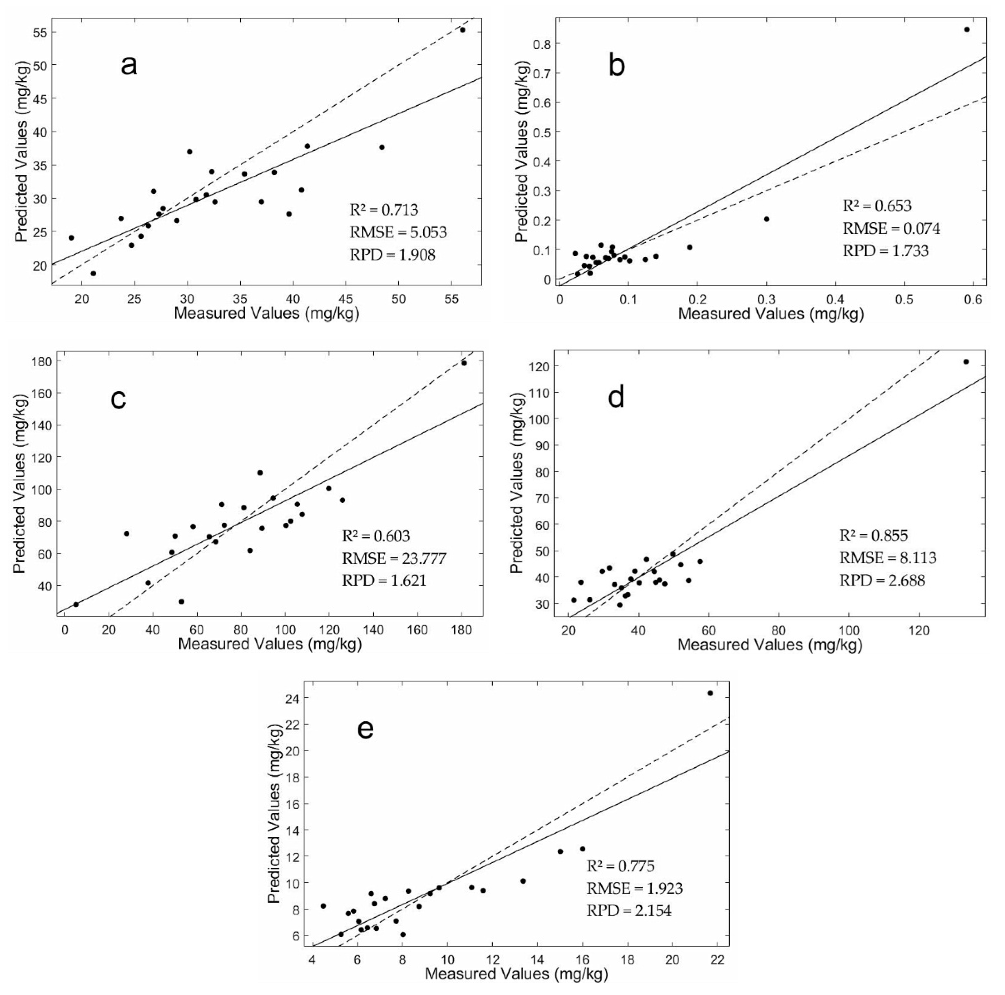
Compared with the single-band model, the model accuracy significantly increased. In the single-band model, except for Hg, Cu, and As contents, Ni and Cr contents could be estimated, but the model accuracy was low, with ${\mathrm{R}}^2$ of 0.424 and 0.361, respectively. The results showed that the modeling accuracy can be significantly improved by using the optimized spectral indices because they can effectively reduce the influence of background noise, and can detect more detailed spectral characteristics. The optimal spectral indices well-magnified the correlation between dependent and independent variables, thus highlighting some important information useful for heavy metal(loid) estimation. Therefore, the optimal spectral indices could effectively compensate for the deficiency of the full-band and characteristic-band methods. Wavelength interaction could also be considered to reduce the influence of irrelevant wavelengths and deal with the overlapping absorption of soil components [70,71,72], showing the potential for estimating the content of heavy metal(loid)s in soil by spectral indices.

This study showed that the optimal spectral indices can be successfully used to estimate the content of heavy metal(loid)s in agricultural soils, and the precision of modeling can be markedly improved. Among the prediction models of soil heavy metal(loid) contents established by the MLR, PLSR, RFR, and ANFIS algorithms, MLR is the most commonly used model because of its clarity and simple structure [73,74,75]. However, compared with MLR, the second generation of the PLSR algorithm has better predictive ability. MLR is a combination of principal component analysis and multiple linear regression, reducing the advantages of variable constraints. Independent variables are used in the PLSR algorithm, which can effectively eliminate the influence of noise, thereby improving the model prediction ability [76,77,78]. In this study, two relatively new machine learning algorithms (RFR and ANFIS) were also adopted, but their model accuracy was significantly lower than those of MLR and PLSR. The main reason may be that a linear relationship exists between the optimized spectral indices used in this study and the soil Ni, Hg, Cr, Cu, and As contents; some studies also reported a significant linear correlation between the spectral band and the content of heavy metal(loid)s [79]. Although RFR and ANFIS algorithms have excellent performance, efficiency, and excellent performance in solving complex nonlinear problems, they tend to lack generalization ability [80,81]. The small sample size is another possible reason limiting the prediction accuracy of the RFR algorithm in this study. By analyzing the accuracy of different models, we found that the optimal spectral indices can weaken nonlinear relationships and enhance linear relationships, improving the prediction accuracy of the model. Therefore, estimating soil heavy metal(loid) contents using optimal spectral indices is feasible, which provides technical support for the rapid monitoring of soil heavy metal(loid) contents.

Our research object was the soil sample point, and the research scope may have some limitations. In future studies, we hope that hyperspectral satellite and UAV remote sensing data can be fully used to obtain soil heavy metal(loid) estimation results in the region. Based on these methods, other substances (such as nitrogen, phosphorus, and potassium) could also be included in a study, which could provide a basis for comprehensive detection and protection of soil. Although we obtained good estimation results in this study, only 92 soil samples were used to develop and verify the model. This small number of soil samples may have affected the stability of the model, and more samples are needed to further improve the model. Some problems have not yet been explored and solved in practical application, such as the influence of soil thickness, soil moisture, soil temperature, and different soil properties on the spectrum, and the correlation between noninteger differential spectra and heavy metal(loid) contents in soil. To summarize, the quantitative modeling of soil heavy metal(loid)s using spectral remote sensing still needs further study. Finally, it is hoped that this study could provide a theoretical basis for the sustainable development of agriculture.

5. Conclusions

In the past, few studies have used the optimal spectral indices to predict the content of heavy metal(loid)s in agricultural soils. Taking Ni, Hg, Cr, Cu, and As in the agricultural soil of the Suzi River Basin, Liaoning Province as an example, we studied the potential of using optimal spectral indices to estimate the contents of Ni, Hg, Cr, Cu, and As in agricultural soil. The results showed that the correlation between the spectrum after mathematical conversion and the Ni, Hg, Cr, Cu, and As contents in agricultural soil is significantly stronger than that of the original spectra, which indicates that spectral processing technology is an effective method to eliminate noise and highlight spectral characteristics, being essential in the spectral analysis process. The correlation between the optimal spectral indices and the contents of Ni, Hg, Cr, Cu, and As in agricultural soils showed that the optimal band combination algorithm could effectively avoid the influence of noise. By using MLR, PLSR, RFR, and ANFIS algorithms to estimate the Ni, Hg, Cr, Cu, and As contents in the soil, we found a strong linear relationship between the optimized spectral indices and the Ni, Hg, Cr, Cu, and As contents in agriculture soil; the Ni, Hg, Cr, Cu, and As contents could be better estimated by MLR and PLSR. The results showed that the introduction of more spectral indices could weaken the nonlinear relationships and enhance the linear relationships and could quickly and accurately estimate the contents of Ni, Hg, Cr, Cu, and As in farmland soil. In addition, this study has some limitations. The influence of different soil types, soil temperature, and other conditions on the spectrum was not considered in the study. More sample data are needed to test the stability of the model. Therefore, in future work, more samples of different soil types will be collected to establish a more scientific and reliable estimation model of soil heavy metal(loid)s. This study’s findings are sufficient to provide a feasible reference for the estimation of heavy metal(loid) contents in other regions or for the estimation of the content of other heavy metal(loid)s, and it provides a theoretical basis for the estimation of metal(loid) contents in soil using hyperspectral satellites, which has strong promotion value. This study also provides technical support for sustainable agricultural development.

References

1. Keesstra, S.D.; Bouma, J.; Wallinga, J.; Tittonell, P.; Smith, P.; Cerdà, A.; Montanarella, L.; Quinton, J.N.; Pachepsky, Y.; van der Putten, W.H.; et al. The significance of soils and soil science towards realization of the United Nations Sustainable Development Goals. Soil 2016, 2, 111–128. [Google Scholar] [CrossRef] [Green Version]
2. Song, Y.; Zhao, X.; Su, H.; Li, B.; Hu, Y.; Cui, X. Predicting Spatial Variations in Soil Nutrients with Hyperspectral Remote Sensing at Regional Scale. Sensors 2018, 18, 3086. [Google Scholar] [CrossRef] [Green Version]
3. Shi, T.; Yang, C.; Liu, H.Z.; Wu, C.; Wang, Z.H.; Li, H.; Zhang, H.F.; Guo, L.; Wu, G.F.; Su, F.Z. Mapping lead concentrations in urban topsoil using proximal and remote sensing data and hybrid statistical approaches. Environ. Pollut. 2021, 272, 116041. [Google Scholar] [CrossRef] [PubMed]
4. Yenilmez, F.; Kuter, N.; Emil, M.K.; Aksoy, A. Evaluation of pollution levels at an abandoned coal mine site in turkey with the aid of gis. Int. J. Coal Geol. 2011, 86, 12–19. [Google Scholar] [CrossRef]
5. Hou, L.; Li, X.; Li, F. Hyperspectral-based Inversion of Heavy Metal Content in the Soil of Coal Mining Areas. J. Environ. Qual. 2019, 48, 57–63. [Google Scholar] [CrossRef] [Green Version]
6. Bhuiyan, M.A.; Parvez, L.; Islam, M.; Dampare, S.B.; Suzuki, S. Heavy metal pollution of coal mine-affected agricultural soils in the northern part of Bangladesh. J. Hazard. Mater. 2010, 173, 384–392. [Google Scholar] [CrossRef] [PubMed]
7. Kemper, T.; Sommer, S. Estimate of heavy metal contamination in soils after a mining accident using reflectance spectroscopy. Environ. Sci. Technol. 2002, 36, 2742. [Google Scholar] [CrossRef]
8. Ferrier, G. Application of imaging spectrometer data in identifying environmental pollution caused by mining at Rodaquilar, Spain. Remote Sens. Environ. 1999, 68, 125–137. [Google Scholar] [CrossRef]
9. Shi, T.Z.; Guo, L.; Chen, Y.Y.; Wang, W.X.; Shi, Z.; Li, Q.Q.; Wu, G.F. Proximal and remote sensing techniques for mapping of soil contamination with heavy metals. Appl. Spectrosc. Rev. 2018, 53, 783–805. [Google Scholar] [CrossRef]
10. Shi, T.; Chen, Y.; Liu, Y.; Wu, G. Visible and near-infrared reflectance spectroscopy an alternative for monitoring soil contamination by heavy metals. J. Hazard. Mater. 2014, 265, 166–176. [Google Scholar] [CrossRef]
11. Tan, K.; Ma, W.B.; Wu, F.Y.; Du, Q. Random forest–based estimation of heavy metal concentration in agricultural soils with hyperspectral sensor data. Environ. Monit. Assess. 2019, 191, 446–459. [Google Scholar] [CrossRef] [PubMed]
12. Sawut, R.; Kasim, N.; Abliz, A.; Li, H.; Yalkun, A.; Maihemuti, B.; Shi, Q.D. Possibility of optimized indices for the assessment of heavy metal contents in soil around an open pit coal mine area. Int. J. Appl. Earth Obs. 2018, 73, 14–15. [Google Scholar] [CrossRef]
13. Wang, J.J.; Cui, L.J.; Gao, W.X.; Shi, T.Z.; Chen, Y.Y.; Gao, Y. Prediction of low heavy metal concentrations in agricultural soils using visible and near-infrared reflectance spectroscopy. Geoderma 2014, 216, 1–9. [Google Scholar] [CrossRef]
14. Zhang, S.W.; Shen, Q.; Nie, C.J.; Huang, Y.F.; Wang, J.H.; Hu, Q.Q.; Ding, X.J.; Zhou, Y.; Chen, Y.P. Hyperspectral inversion of heavy metal content in reclaimed soil from a mining wasteland based on different spectral transformation and modeling methods. Spectrochim. Acta. A. 2019, 211, 393–400. [Google Scholar] [CrossRef]
15. Hong, Y.S.; Shen, R.L.; Cheng, H.; Chen, S.C.; Chen, Y.Y.; Guo, L.; He, J.H.; Liu, Y.L.; Yu, L.; Liu, Y. Cadmium concentration estimation in peri-urban agricultural soils: Using reflectance spectroscopy, soil auxiliary information, or a combination of both? Geoderma 2019, 354, 113875. [Google Scholar] [CrossRef]
16. Gholizadeh, A.; Žižala, D.; Saberioon, M.; Boruvka, L. Soil organic carbon and texture retrieving and mapping using proximal, airborne and Sentinel-2 spectral imaging. Remote Sens. Environ. 2018, 218, 89–103. [Google Scholar] [CrossRef]
17. Zhou, W.; Yang, H.; Xie, L.Y.; Li, H.R.; Huang, L.; Zhao, Y.P.; Yue, T.X. Hyperspectral inversion of soil heavy metals in Three-River Source Region based on random forest model. Catena 2021, 202, 105222. [Google Scholar] [CrossRef]
18. Wei, L.F.; Pu, H.C.; Wang, Z.X.; Yuan, Z.R.; Yan, X.R.; Cao, L.Q. Estimation of Soil Arsenic Content with Hyperspectral Remote Sensing. Sensors 2020, 20, 4056. [Google Scholar] [CrossRef]
19. Bilgili, A.V.; Akbas, F.; Es, H. Combined use of hyperspectral VNIR reflectance spectroscopy and kriging to predict soil variables spatially. Precis. Agric. 2011, 12, 395–420. [Google Scholar] [CrossRef]
20. Soriano-Disla, J.M.; Janik, L.J.; Rossel, R.A.V.; Macdonald, L.M.; McLaughlin, M.J. The performance of visible, near-, and mid-infrared reflectance spectroscopy for prediction of soil physical, chemical, and biological properties. Appl. Spectrosc. Rev. 2014, 49, 139–186. [Google Scholar] [CrossRef]
21. Sun, W.; Zhang, X. Estimating soil zinc concentrations using reflectance spectroscopy. Int. J. Appl. Earth Obs. Geoinf. 2017, 58, 126–133. [Google Scholar] [CrossRef]
22. Tariq, F.; Wang, X.K.; Saleem, M.H.; Khan, Z.I.; Ahmad, K.; Malik, I.S.; Munir, M.; Mahpara, S.; Mehmood, N.; Ahmad, T.; et al. Risk Assessment of Heavy Metals in Basmati Rice: Implications for Public Health. Sustainability 2021, 13, 8513. [Google Scholar] [CrossRef]
23. Zhang, Z.Y.; Mamat, A.; Simayi, Z. Pollution assessment and health risks evaluation of (metalloid) heavy metals in urban street dust of 58 cities in China. Environ. Sci. Pollut. R. 2019, 26, 126–140. [Google Scholar] [CrossRef] [PubMed]
24. Yin, G.C.; Zhu, H.H.; Chen, Z.L.; Su, C.H.; He, Z.C.; Chen, X.L.; Qiu, J.R.; Wang, T.Y. Spatial Distribution and Source Apportionment of Soil Heavy Metals in Pearl River Delta, China. Sustainability 2021, 13, 9651. [Google Scholar] [CrossRef]
25. Sui, S.F.; Ng, J.; Gao, Y.X.; Peng, C.; He, C.; Wang, G.L.; Liu, Z.Y. Pollution characteristics and chronic health risk assessment of metals and metalloids in ambient PM 2.5 in Licheng District, Jinan, China. Environ. Geochem. Health 2020, 42, 1803–1815. [Google Scholar] [CrossRef]
26. Najafi, S.H.; Maryam, P.; Mahmood, Y.; Baghal, A.F.; Gea, O.C.; Elham, T.; Akbar, M.A. Carcinogenic and Non-carcinogenic Risk Assessment of Heavy Metals in Groundwater Wells in Neyshabur Plain, Iran. Biol. Trace Elem. Res. 2019, 190, 251–261. [Google Scholar]
27. Abdul, K.S.M.; Jayasinghe, S.S.; Chandana, E.P.S.; Jayasumana, C.; De, S.P.M.C.S. Arsenic and human health effects: A review. Environ. Toxicol. Phar. 2015, 40, 828–846. [Google Scholar] [CrossRef]
28. He, X.D.; Li, P.Y.; Ji, Y.J.; Wang, Y.H.; Su, Z.M.; Elumalai, V. Groundwater Arsenic and Fluoride and Associated Arsenicosis and Fluorosis in China: Occurrence, Distribution and Management. Expos. Health 2020, 12, 355–368. [Google Scholar] [CrossRef]
29. Eslami, H.; Esmaeili, A.; Razaeian, M.; Salari, M.; Hosseini, A.N.; Mobini, M.; Barani, A. Potentially toxic metal concentration, spatial distribution, and health risk assessment in drinking groundwater resources of southeast Iran. Geosci. Front. 2022, 13, 101276. [Google Scholar] [CrossRef]
30. Wang, Q.; Xie, Z.; Li, F. Using ensemble models to identify and apportion heavy metal pollution sources in agricultural soils on a local scale. Environ. Pollut. 2015, 206, 227–235. [Google Scholar] [CrossRef]
31. Tan, K.; Wang, H.M.; Chen, L.H.; Du, Q.; Du, P.J.; Pan, C.C. Estimation of the spatial distribution of heavy metal in agricultural soils using airborne hyperspectral imaging and random forest. J. Hazard. Mater. 2020, 382, 120987.1–120987.13. [Google Scholar] [CrossRef] [PubMed]
32. He, M.; Wang, Z.; Tang, H. The chemical, toxicological and ecological studies in assessing the heavy metal pollution in Le’an River, China. Water Res. 1998, 32, 510–518. [Google Scholar] [CrossRef]
33. Liu, W.X.; Coveney, R.M.; Chen, J.L. Environmental quality assessment on a river system polluted by mining activities. Appl. Geochem. 2003, 18, 749–764. [Google Scholar] [CrossRef]
34. National Environmental Protection Standards of the People’s Republic of China (HJ 781-2016); Ministry of Environmental Protection of the People’s Republic China: Beijing, China, 2016. Available online: https://www.chinesestandard.net/PDF/English.aspx/HJ781-2016 (accessed on 1 March 2016).
35. Soil Quality—Analysis of Total Mercury, Arsenic and Lead Contents. Atomic Fluorescence Spectrometry—Part 1: Analysis of Total Mercury Contents in Soils; General Administration of Quality Supervision, Inspection and Quarantine of the People’s Republic of China, Standardization Administration of the People’s Republic of China: Beijing, China, 2008. Available online: http://std.samr.gov.cn/gb/search/gbDetailed?id=5DDA8BA1C8A318DEE05397BE0A0A95A7 (accessed on 1 June 2021).
36. Liu, Y.L.; Chen, H.; Wu, G.F.; Wu, X.G. Feasibility of estimating heavy metal concentrations in Phragmites australis using laboratory-based hyperspectral data—A case study along Le’an River, China. Int. J. Appl. Earth Obs. 2010, 12, 0303–2434. [Google Scholar] [CrossRef]
37. Pandit, C.M.; Filippelli, G.M.; Li, L. Estimation of heavy-metal contamination in soil using reflectance spectroscopy and partial least-squares regression. Int. J. Remote Sens. 2010, 31, 4111–4123. [Google Scholar] [CrossRef]
38. Gomez, C.; Viscarra Rossel, R.A.; McBratney, A.B. Soil organic carbon reduction by hyperspectral remote sensing and field vis–NIR spectroscopy: An Australian case study. Geoderma 2008, 146, 403–411. [Google Scholar] [CrossRef]
39. Jiang, Z.; Fei, B.; Yang, Z. The effect of spectral pretreatment on the prediction of wood cellulose crystallinity by near infrared spectroscopy. Spectrosc. Spectr. Anal. 2007, 27, 435–438. [Google Scholar]
40. Zhao, Y.X.; Yan, C.H.; Lu, S.; Wang, P.; Qiu, G.Y.; Li, R.L. Estimation of chlorophyll content in intertidal mangrove leaves with different thicknesses using hyperspectral data. Ecol. Indic. 2019, 106, 105511. [Google Scholar] [CrossRef]
41. Liu, Z.H.; Lu, Y.; Peng, Y.P.; Zhao, L.; Wang, G.X.; Hu, Y.M. Estimation of Soil Heavy Metal Content Using Hyperspectral Data. Remote Sens. 2019, 11, 1464. [Google Scholar] [CrossRef] [Green Version]
42. Chagas, C.D.S.; Junior, W.D.C.; Bhering, S.B.; Filho, B.C. Spatial prediction of soil surface texture in a semiarid region using random forest and multiple linear regressions. Catena 2016, 139, 232–240. [Google Scholar] [CrossRef]
43. Zhang, H.; Wu, P.B.; Yin, A.J.; Yang, X.H.; Zhang, M.; Gao, C. Prediction of soil organic carbon in an intensively managed reclamation zone of eastern China: A comparison of multiple linear regressions and the random forest model. Sci. Total Environ. 2017, 592, 704–713. [Google Scholar] [CrossRef] [PubMed]
44. Xie, X.F.; Wu, T.; Zhu, M.; Jiang, G.J.; Xu, Y.; Wang, X.H.; Pu, L.J. Comparison of random forest and multiple linear regression models for estimation of soil extracellular enzyme activities in agricultural reclaimed coastal saline land. Ecol. Indic. 2021, 120, 106925. [Google Scholar] [CrossRef]
45. Wold, H. Nonlinear Estimation by Iterative Least Squares Procedure. In Research Papers in Statistics; David, F., Ed.; Wiley & Sons: New York, NY, USA, 1966; pp. 411–444. [Google Scholar]
46. Zhang, Q.; Zhou, B.B.; Li, M.J.; Wei, Q.P.; Han, Z.H. Multivariate analysis between meteorological factor and fruit quality of Fuji apple at different locations in China. J. Integr. Agric. 2018, 17, 1338–1347. [Google Scholar] [CrossRef]
47. Mirzaei, M.; Marofi, S.; Abbasi, M.; Solgi, E.; Karimi, R.; Verrelst, J. Scenario-based discrimination of common grapevine varieties using in-field hyperspectral data in the western of Iran. Int. J. Appl. Earth Obs. Geoinf. 2019, 80, 26–37. [Google Scholar] [CrossRef]
48. Breiman, L. Random forests. Mach. Learn. 2001, 45, 5–32. [Google Scholar] [CrossRef] [Green Version]
49. Immitzer, M.; Atzberger, C.; Koukal, T. Tree species classification with random forest using very high spatial resolution 8-band Worldview-2 satellite data. Remote Sens. 2012, 4, 2661–2693. [Google Scholar] [CrossRef] [Green Version]
50. Rodriguez-Galiano, V.F.; Ghimire, B.; Rogan, J.; Chica-Olmo, M.; Rigol-Sanchez, J.P. An assessment of the effectiveness of a random forest classifier for land-cover classification. ISPRS J. Photogramm. Remote Sens. 2012, 67, 93–104. [Google Scholar] [CrossRef]
51. Singh, T.N.; Sinha, S.; Singh, V.K. Prediction of thermal conductivity of rock through physico-mechanical properties. Build. Environ. 2007, 42, 146–155. [Google Scholar] [CrossRef]
52. Hosseini, M.; Agereh, S.R.; Khaledian, Y.; Zoghalchali, J.H.; Brevik, E.C.; Naeini, M.S.A.R. Comparison of multiple statistical techniques to predict soil phosphorus. Appl. Soil Ecol. 2017, 114, 123–131. [Google Scholar] [CrossRef]
53. Rahmanian, B.; Pakizeh, M.; Mansoori, S.A.A.; Esfandyari, M.; Jafari, D.; Maddah, H.; Maskooki, A. Prediction of MEUF process performance using artificial neural networks and ANFIS approaches. J. Taiwan Inst. Chem. E. 2012, 43, 558–565. [Google Scholar] [CrossRef]
54. Tan, K.; Ma, W.B.; Chen, L.H.; Wang, H.M.; Du, Q.; Du, P.J.; Yan, B.K.; Liu, R.Y.; Li, H.D. Estimating the Distribution Trend of Soil Heavy Metals in Mining Area from HyMap Airborne Hyperspectral Imagery Based on Ensemble Learning. J. Hazard. Mater. 2020, 123288. [Google Scholar] [CrossRef]
55. Manta, D.S.; Angelone, M. Heavy metals in urban soils: A case study from the city of Palermo (Sicily), Italy. Sci. Total Environ. 2002, 300, 229–243. [Google Scholar] [CrossRef]
56. Chen, Z.L.; Yin, W.Y.; Liu, H.T.; Liu, Q.; Yang, Y. Review of Monitoring Petroleum-Hydrocarbon Contaminated Soils with Visible and Near-Infrared Spectroscopy. Spectrosc. Spectr. Anal. 2017, 37, 1723–1727. [Google Scholar]
57. Khosravi, V.; Ardejani, F.D.; Yousefi, S.; Aryafar, A. Monitoring soil lead and zinc contents via combination of spectroscopy with extreme learning machine and other data mining methods. Geoderma 2018, 318, 29–41. [Google Scholar] [CrossRef]
58. Chakraborty, S.; Weindorf, D.C.; Deb, S.; Li, B.; Paul, S.; Choudhury, A.; Ray, D.P. Rapid assessment of regional soil arsenic pollution risk via diffuse reflectance spectroscopy. Geoderma 2017, 289, 72–81. [Google Scholar] [CrossRef]
59. Jiang, J.J.; Xu, J.; He, J.L.; Cai, H.L.; Zhang, C.Y. Method for retrieving soil cadmium content based on organic matter diagnostic index. Acta Pedol. Sin. 2009, 46, 177–182. [Google Scholar]
60. Rossel, R.V.; Behrens, T. Using data mining to model and interpret soil diffuse reflectance spectra. Geoderma 2010, 158, 46–54. [Google Scholar] [CrossRef]
61. Lu, Q.; Wang, S.J.; Bai, X.Y.; Liu, F.; Wang, M.M.; Wang, J.F.; Tian, S.Q. Rapid inversion of heavy metal concentration in karst grain producing areas based on hyperspectral bands associated with soil components. Microchem. J. 2019, 148, 404–411. [Google Scholar] [CrossRef]
62. Stazi, S.R.; Antonucci, F.; Pallottino, F.; Costa, C.; Marabottini, R.; Petruccioli, M.; Menesatti, P. Hyperspectral visible–near infrared determination of arsenic concentration in soil. Commun. Soil Sci. Plan. 2014, 45, 2911–2920. [Google Scholar] [CrossRef]
63. Shen, Q.; Xia, K.; Zhang, S.W.; Kong, C.C.; Hu, Q.Q.; Yang, S.W. Hyperspectral indirect inversion of heavy-metal copper in reclaimed soil of iron ore area. Spectrochim. Acta. A 2019, 222, 117191. [Google Scholar] [CrossRef] [PubMed]
64. Viscarra, R.R.A.; Walvoort, D.J.J.; McBratney, A.B.; Janik, L.J.; Skjemstad, J.O. Visible, near infrared, mid infrared or combined diffuse reflectance spectroscopy for simultaneous assessment of various soil properties. Geoderma 2007, 131, 59–75. [Google Scholar] [CrossRef]
65. Berg, A.; Sheffield, J.; Milly, P.C.D. Divergent surface and total soil moisture projections under global warming. Geophys. Res. Lett. 2017, 44, 236–244. [Google Scholar] [CrossRef] [Green Version]
66. Maleki, M.R.; VanHolm, L.; Ramon, H.; Merckx, R.; DeBaerdemaeker, J.; Mouazen, A.M. Phosphorus Sensing for Fresh Soils using Visible and Near Infrared Spectroscopy. Biosyst. Eng. 2006, 95, 425–436. [Google Scholar] [CrossRef]
67. Barnes, R.J.; Dhanoa, M.S.; Lister, S.J. Standard normal variate transformation and de-trending of near-infrared diffuse reflectance spectra. Appl. Spectrosc. 2016, 43, 772–777. [Google Scholar] [CrossRef]
68. Xu, X.T.; Chen, S.B.; Xu, Z.Y.; Yu, Y.; Zhang, S.; Dai, R. Exploring Appropriate Preprocessing Techniques for Hyperspectral Soil Organic Matter Content Estimation in Black Soil Area. Remote Sens. 2020, 12, 3765. [Google Scholar] [CrossRef]
69. Liu, M.L.; Liu, X.N.; Ding, W.C.; Wu, L. Monitoring stress levels on rice with heavy metal pollution from hyperspectral reflectance data using wavelet-fractal analysis. Int. J. Appl. Earth Obs. 2011, 13, 246–255. [Google Scholar] [CrossRef]
70. Nawar, S.; Buddenbaum, H.; Hill, J. Estimation of soil salinity using three quantitative methods based on visible and near-infrared reflectance spectroscopy: A case study from Egypt. Arab. J. Geoences 2015, 8, 5127–5140. [Google Scholar] [CrossRef]
71. Bao, N.; Wu, L.; Ye, B.; Yang, K.; Zhou, W. Assessing soil organic matter of reclaimed soil from a large surface coal mine using a field spectroradiometer in laboratory. Geoderma 2017, 288, 47–55. [Google Scholar] [CrossRef]
72. Shi, T.Z.; Liu, H.Z.; Chen, Y.Y.; Wang, J.J.; Wu, G.F. Estimation of arsenic in agricultural soils using hyperspectral vegetation indices of rice. J. Hazard. Mater. 2016, 308, 243–252. [Google Scholar] [CrossRef]
73. Li, X.Q.; Li, L.; Liu, X.N. Collaborative inversion heavy metal stress in rice by using two-dimensional spectral feature space based on HJ-1 A HSI and radarsat-2 SAR remote sensing data. Int. J. Appl. Earth Obs. 2019, 78, 39–52. [Google Scholar] [CrossRef]
74. Kooistra, L.; Leuven, R.S.E.W.; Wehrens, R.; Nienhuis, P.H.; Buydens, L.M.C. A comparison of methods to relate grass reflectance to soil metal contamination. Int. J. Remote Sens. 2003, 24, 4995–5010. [Google Scholar] [CrossRef]
75. Mirzaei, M.; Verrelst, J.; Marofi, S.; Abbasi, M.; Azadi, H. Eco-Friendly Estimation of Heavy Metal Contents in Grapevine Foliage Using In-Field Hyperspectral Data and Multivariate Analysis. Remote Sens. 2019, 11, 2731. [Google Scholar] [CrossRef] [Green Version]
76. Abrougui, K.; Gabsi, K.; Mercatoris, B.; Khemis, C.; Amami, R.; Chehaibi, S. Prediction of organic potato yield using tillage systems and soil properties by artificial neural network (ANN) and multiple linear regressions (MLR). Soil Till. Res. 2019, 190, 202–208. [Google Scholar] [CrossRef]
77. Abdi, H. Partial least squares regression and projection on latent structure regression (PLS regression). Wiley Interdiscip. Rev. Comput. Stat. 2010, 2, 97–106. [Google Scholar] [CrossRef]
78. Carrascal, L.M.; Galvan, I.; Gordo, O. Partial least squares regression as an alternative to current regression methods used in ecology. Oikos 2009, 118, 681–690. [Google Scholar] [CrossRef]
79. Zhou, X.; Sun, J.; Tian, Y.; Chen, Q.S.; Wu, X.H.; Hang, Y.Y. A deep learning based regression method on hyperspectral data for rapid prediction of cadmium residue in lettuce leaves. Chemometr. Intell. Lab. 2020, 200, 103996. [Google Scholar]
80. Singh, A.; Jakubowski, A.R.; Chidister, I.; Townsend, P.A. A MODIS approach to predicting stream water quality in Wisconsin. Remote Sens. Environ. 2013, 128, 74–86. [Google Scholar] [CrossRef]
81. Zhou, X.; Sun, J.; Tian, Y.; Lu, B.; Hang, Y.Y.; Chen, Q.S. Hyperspectral technique combined with deep learning algorithm for detection of compound heavy metals in lettuce. Food Chem. 2020, 321, 126503. [Google Scholar] [CrossRef] [PubMed]
Figure 1. Map of the study area.
Sustainability 13 12088 g001
Figure 2. Reflectance spectra of 92 soil samples: (A) the original spectra; (B) those processed by piecewise SG smoothing.
Sustainability 13 12088 g002
Figure 3. Spectral transformation curves of soil: (a) CR; (b) 1/R; (c) FDR; (d) SDR; and (e) R .
Sustainability 13 12088 g003aSustainability 13 12088 g003b
Figure 4. Pearson correlation coefficients between the soil Ni, Hg, Cr, Cu, and As contents and spectra for: (a) OR; (b) CR; (c) 1/R; (d) FDR; (e) SDR; and (f) R (p = 0.01).
Sustainability 13 12088 g004aSustainability 13 12088 g004b
Figure 5. Scatterplots illustrating the optimal accuracy of Ni, Hg, Cr, Cu, and As: (a) Ni, SDR partial least-squares regression (MLR) model; (b) Hg, SDR partial least-squares regression (PLSR) model; (c) Cr, SDR partial least-squares regression (PLSR) model; (d) Cu, FDR multiple linear regression (MLR)model; and (e) As, SDR partial least-squares regression (PLSR) model. The solid line is the regression line between the estimated and measured values, and the dashed line is the 1:1 line.
Sustainability 13 12088 g005