
Electricity Consumption in China: The Effects of Financial Development and Trade Openness


School of Economics and Commerce, Henan University of Technology, Zhengzhou 450001, China
*
Author to whom correspondence should be addressed.
Sustainability 2021, 13(18), 10206; https://doi.org/10.3390/su131810206
Submission received: 13 August 2021
/
Revised: 4 September 2021
/
Accepted: 8 September 2021
/
Published: 13 September 2021
Abstract
:As China is facing the double pressure of economic growth as well as energy-saving and reduction of emissions, reducing electricity consumption without affecting economic development is a challenging and critical issue. Based on 31 provincial panel’s data in China from 2004 to 2018, this study empirically analyzes the direction and degree of the impact of financial development and trade openness on electricity consumption using the spatial econometric approach and panel vector autoregression (PVAR) model. The results indicate that China’s electricity consumption presents a significant spatial spill over effect, and the spatial agglomeration of electricity consumption in local regions is mainly HH clusters. A 1% positive change in financial development causes an increase of 0.089% in electricity consumption, but a 1% rise in financial development reduces electricity consumption of neighboring regions by 0.051%. A 1% positive change in trade openness decreases electricity consumption by 0.051%, while the spatial spillover effect of trade openness is not significant. It is also found that financial development has a long-term promoting effect on electricity consumption, while trade openness has a long-term inhibiting effect on electricity consumption.
1. Introduction
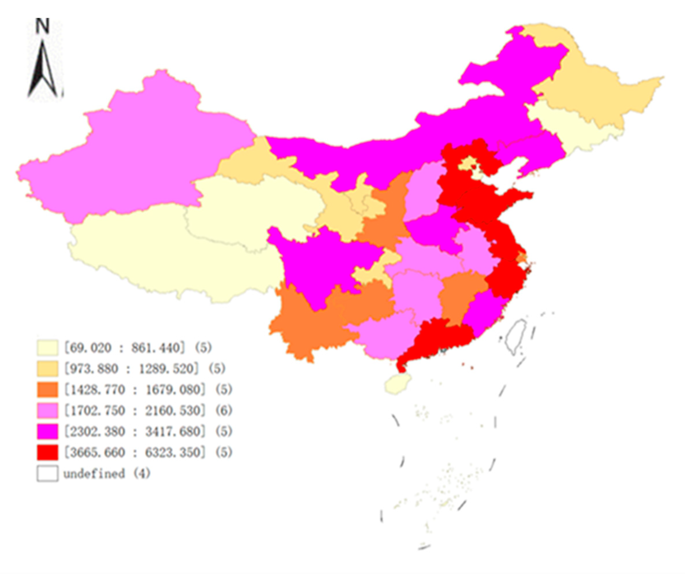
Electricity is the fastest-growing source of final energy consumption, and global electricity demand grows at 2.1% per year from 2018 to 2040, twice the rate of primary energy demand. The environmental implications of these patterns of energy use are stark, and energy-related CO2 emissions hit a record high since 2013 with a 1.9% increase in 2018 [1]. Due to the heavy dependence on fossil fuels, world electricity generation leads to massive carbon emissions, which accounts for 37.5% of total CO2 emissions [2]. China is the world’s largest CO2 emitter, with 9570.8 Mt of CO2 emissions in 2018, occupying 28.6% of world emissions [3]. China is actively pursuing a decarbonization transition, with the government committing to a carbon peak by 2030 and net-zero emissions by 2060. Figure 1 shows the regional distribution of electricity consumption based on six quantile maps in 2018. The five provinces with the highest value of electricity consumption are Hebei, Jiangsu, Zhejiang, Shandong, and Guangdong. The maximum value appeared in Guangdong province, where the corresponding electricity consumption is 632.34 billion kWh. Indeed, due to economic development, geographic environment, and consequent population distribution, the electricity consumptions of eastern provinces are higher than the central and western provinces. Specifically, the average electricity consumption in eastern, central, and western provinces is 216 billion kWh, 124.6 billion kWh, and 95.1 billion kWh, respectively (three regional division methods can be found in [4]).
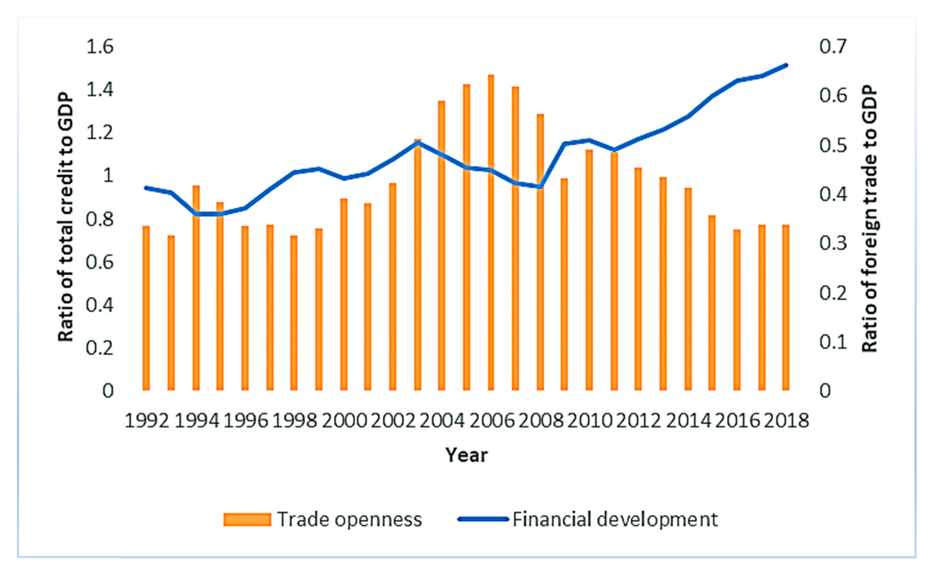
Financial development is one possible way to increase economic growth, and this will affect energy demand. After accession to the World Trade Organization (WTO), China has continued to improve its multi-level and multi-functional financial market system, and its banking transactions and information system services help increase the ratio of bank loans to GDP. Figure 2 shows that between 1992 and 2018, the ratio of total loans from financial institutions to GDP from 0.95 in 1992 to 1.51 in 2018. Financial development can impact the demand for electricity through four different channels. First, financial development can make it easier for consumers to borrow money to buy big ticket items such as cars, houses, refrigerators, air conditioners, and washing machines. These commodities typically consume large amounts of electricity, which can affect a country’s overall demand for electricity. Second, businesses also benefit from improved financial development because it makes it easier and less costly to gain access to financial capital to expand existing businesses or create new ones. Third, the stock market creates a wealth effect that boosts consumer and business confidence, and increased economic confidence stimulates the demand for energy-intensive products [5]. Fourth, financial development can promote technological innovation and improve power efficiency. A developed financial market can provide financing support for green power projects, thereby promoting the upgrading of electricity structure [6].
Regarding trade openness, after 1978, China gradually relaxed from central planning and opened up for trade [7]. China became a member of the WTO in 2001, which further accelerated the process of China’s integration into the global economy. Figure 2 indicates that foreign trade as a share of GDP improved dramatically from 33.53% in 1992 to 64.24% in 2006 before taking a dip to 33.88% in 2018. The common opinion about trade openness is that it leads to an increase in economic output and, therefore, to an increase in energy consumption. However, Sbia et al. [8] argued that free trade may lead to an increase in energy use efficiency because of larger energy markets and easier access to low-energy products. Their study revealed that a 0.3631% energy demand is declined by a 1% increase in trade openness in the United Arab Emirates.
This paper contributes to the existing literature in three aspects: First, few studies explain electricity consumption by putting financial development and trade openness together. This paper incorporates financial development and trade openness into a unified analysis framework to describe the effects of these two factors on electricity demand, which can be regarded as a very useful supplement to the existing research. Second, most empirical studies on electricity consumption are based on the assumption of spatial independence. According to Tobler’s first law of geography, certain economic behaviors in a given area may be influenced by neighboring areas, and the attributes of spatial objects in adjacent geographical locations tend to be similar [9]. This study applies spatial econometric approaches to reveal the temporal-spatial distribution characteristics of China’s electricity consumption, as well as the direct and spatial spillover effects of financial development and trade openness on electricity consumption. Third, this paper uses the PVAR model to empirically analyze the impact of financial development and trade openness on electricity consumption. The advantage of using a PVAR method is that by treating all variables as endogenous, the PVAR model contributes to alleviating the endogeneity problem. Furthermore, the impulse response function based on the PVAR approach can account for the response of deviations to shocks in other variables in the long-run, whereas panel regression cannot capture such a dynamic effect.
2. Literature Review
The existing studies show that a great variety of factors can affect electricity consumption [6,9,10,11,12,13,14,15,16,17,18]. Sadorsky [10] explored the linkage between information communication technology and electricity consumption in emerging economies, finding that the use of information communication technology causes an upsurge in the demand for electricity consumption. Salahuddin and Alam [12] concluded that Internet usage and economic growth have no significant short-run relationship with electricity consumption, and there is a unidirectional causal relationship from Internet use to economic growth and electricity consumption. Al-Bajjali and Shamayleh [13] revealed that in Jordan GDP, urbanization, population, structure of economy and aggregate water consumption are significant and positively related to electricity consumption, while electricity prices are significant and negatively related to electricity consumption. Kumari and Sharma [14] analyzed the causal relationship among gross domestic product, foreign direct investment and electricity consumption in India. Lin and Wang [15] explained the inconsistency between electricity consumption and economic growth, pointing out that the feedback effect exists between electricity consumption and economic growth in most regions of China. An et al. [9] figured out that technological progress and optimization of industrial structure are two effective solutions to reduce electricity consumption in China. Zhang et al. [18] explored the impact of temperature on electricity consumption in the Yangtze River Delta Urban Agglomeration from the perspective of income growth, i.e., the moderating effect of income growth on the response of urban residential electricity to temperature changes.
Previous studies have explored the reasons for the rapid growth of electricity consumption from different perspectives, but the impact of financial development on electricity demand is a topic that has received little attention. Rafindadi and Ozturk [19] examined the relationship between economic growth, financial development, capital and trade openness, and electricity consumption in Japan from 1970 to 2012 using an ex-tended Cobb–Douglas production function. The results discover that in the long-run a 1% rise in the financial development will exert considerable pressure on the country’s electricity consumption by 0.2429%. Sbia et al. [20] investigated the relationship between economic growth, urbanization, financial development, and electricity consumption in the United Arab Emirates over the period 1975–2011 using the autoregressive distributed lag (ARDL) bounds test and the Granger causality vector error correction method (VECM). Their empirical findings confirm the existence of the bidirectional causality between financial development and electricity consumption, and financial development adds to electricity consumption. Faisal et al. [21] examined the relationship between internet usage, financial development, economic growth, capital, and electricity consumption by applying the structural break unit root test and the ARDL bounds test to quarterly data from 1993, Q1 to 2014, Q4. The long-run results confirm the existence of an inverted U-shaped relationship between financial development and electricity consumption. Solarin et al. [22] investigated the impact of information and communication technology, financial development and economic growth on electricity consumption by using the electricity demand function in case of Malaysia for the period of 1990–2015. The empirical results validate that financial development increases electricity consumption and the presence of bidirectional causality between financial development and electricity consumption. Adom [23] estimated the effect of financial development on electricity consumption for economies with above and below mean human capital index in 45 African countries using the simultaneous system generalized method of moments (GMM) estimator and the Aiken and West slope difference test. The results reveal that the direct effect of financial development increases electricity consumption, but the indirect effect of financial development reduces electricity consumption. Liu and Li [6] constructed two spatial panel models to explore the interaction between financial development and electricity consumption on the basic panel data of 278 cities in China from 2005 to 2016. The results show financial development is closely related to electricity consumption, urban industrial electricity consumption (IEC), and urban residential electricity consumption (REC), and the elasticity coefficients of financial development to electricity consumption, IEC, and REC are 0.079, 0.061, and 0.244, respectively. Meanwhile, financial development plays an important role in the increase of REC and IEC in eastern regions, western regions, small cities, large cities, and megacities of China.
A number of studies also explore the relationship between trade openness and electricity consumption. Lin et al. [24] employed the Johansen cointegration technique and vector error correction model to analyze the factors influencing renewable electricity consumption in China using data from 1980 to 2011. The results show that there is a long-term relationship between renewable electricity consumption and trade openness, and trade openness undermines renewable electricity consumption. Ohlan [25] explored the relationship between electricity consumption, trade openness, and economic growth in India utilizing ARDL model, Hatemi-J cointegration model, and Granger causality VECM for the period 1971–2016. The results indicate that electricity consumption and trade openness have a long-run association, and they find the existence of a long-term Granger causality flowing from electricity use to trade openness. Gregori and Tiwari [7] employed Pesaran’s CD test, the PANIC and PANICCA approaches, and Granger causality tests to analyze the short- and long-run linkages among electricity consumption, urbanization, GDP, and trade using data for 28 provinces during the period 1995–2016. The results reveal that trade openness displays feedback effects in the short-run, and there is a unidirectional long-run Granger causality running from trade openness to electricity consumption. Ghazouani et al. [26] applied ARDL approach to examine the nexus between trade openness, renewable electricity consumption, and economic growth for seven Asia-Pacific countries over the period 1980–2017. The results demonstrate that trade openness is an important long-run determinant of renewable electricity consumption in Indonesia, Malaysia, and Thailand, and there is evidence of Granger causality running from trade openness to renewable electricity consumption in Indonesia, Malaysia, Pakistan, and South Korea. Sahoo and Sethi [27] applied structural break and cointegration tests to examine the effects of remittance inflow, FDI, trade openness and urbanization on electricity consumption in India during the 1975–2017 period. The results reveal that 1% increase in trade openness leads to increase electricity consumption by 0.0884%.
In summary, the previous literature on financial development, trade openness, and electricity consumption shows that there are still some limitations in this area. First, the past literature has not included financial development, trade openness, and electricity consumption in the same analytical framework for empirical research. Second, most empirical studies on electricity consumption are based on the assumption of spatial independence. It is particularly important to take into account spatial dependencies, and ignoring them can produce biases, inaccuracies, and inconsistencies in the results [28,29]. Third, the previous studies are mostly static analyses, and the endogeneity problem caused by reverse causality could not be effectively addressed [30]. Therefore, this paper applies PVAR method to analyze the dynamic effects of financial development and trade openness on electricity consumption. The advantage of applying the PVAR method is that all variables can be simultaneously treated as endogenous, and thus the PVAR model can effectively address the potential endogeneity problem.
3. Methodology
3.1. Variables and Data
In this paper, the purpose is to discuss the aggregated electricity consumption at the provincial level in China. Therefore, the dependent variable is indicated by the electricity consumption in different provinces, in units of 100 million kWh [7,20]. Two core independent variables are financial development and trade openness. There are many indicators used by researchers as proxies for financial development, which is a complex economic phenomenon that can be studied from different perspectives [31,32]. Following the most commonly proxy adopted in previous studies, this study uses the ratio of total loans to the region’s nominal GDP to measure financial development [20,33]. According to [34,35], trade openness is measured by the proportion of total import and export trade with the use of official exchange rates to the region’s nominal GDP. This study takes economic growth, foreign direct investment, fixed asset investment, industrialization, and urbanization as control variables. The variable definitions are presented in Table 1.
The data cover 31 provinces in China for the period 2004–2018. The data are drawn from the China Statistical Yearbook (2005–2019) and China Financial Yearbook (2005–2019) compiled by the China Bureau of Statistics, as well as the statistical bulletins on national economic and social development of the relevant provinces. All variables are adopted as their natural logarithm to avoid sharpness in the data [20]. The descriptive statistics for each variable are listed in Table 2.

Table 1.
Variable name, symbols, and definitions.
| Variable Name | Symbol | Definition |
|---|---|---|
| Electricity consumption | ec | The amount of electricity consumption in different provinces in units of 108 kWh |
| Financial development | fde | The ratio of total credit to the region’s nominal GDP |
| Trade openness | tro | The proportion of total import and export trade with the use of official exchange rates to the region’s nominal GDP |
| Economic growth | pgdp | Per capita GDP in different provinces [29,36] |
| Foreign direct investment | fdi | Foreign direct investment according to the exchange rate of USD in each year [37,38,39] |
| Fixed asset investment | fai | The ratio of fixed asset investment to the region’s nominal GDP [40] |
| Industrialization | ind | The ratio of industrial value added to the region’s nominal GDP [34,41] |
| Urbanization | urb | The ratio of urban population to the total population [42,43] |
3.2. Panel Unit Root Test
If a series is non-stationary, it may lead to erroneous results before using them for further analysis [44]. For this purpose, this study employs panel unit root tests developed by [45] (hereafter LLC), [46] (hereafter HT) and [47] (hereafter IPS).
The LLC test uses the following panel ADF specification:
where is a vector of endogenous variables; represents panel-specific means and trends; is white noise. The LLC test assumes all panels share the same autoregressive parameters (i.e., for all i). This procedure tests the null hypothesis of a unit root (= 0) versus the alternative hypothesis (). Acceptance of the alternative hypothesis allows the individual series to be integrated.
The HT test statistic is based on the OLS estimator,, in the regression model:
Because the inclusion of panel means and time trends in the model may lead to biased estimates, the null hypothesis is not but .
The IPS test, which is also based on Equation (1), differs from the LLC test by relaxing the assumption of a common autoregressive parameter. The IPS tests the null hypothesis (for all i) against the alternative hypothesis (for all i). Rejection of the null hypothesis indicates no unit root.
3.3. Pedroni Cointegration Test
The purpose of the cointegration test is to examine whether the variables have a stable relationship with each other over time. For each series individually, it is non-stationary, but a linear combination of these series may be stationary. Given the existence of such a linear combination, these non-stationary (with unit roots) series are considered to have a cointegrating relationship with each other [48]. If it is found that the variables are non-stationary at the level and stationary only at first differences (I(1)), then we can conduct cointegration test. Pedroni [49] proposed a residual-based test for the null of cointegration allowing for individual heterogeneous fixed effects and trend terms. Consider the following specification:
where ; The variables and are assumed to be I(1),and the residual will also be I(1); and are fixed effects and time trend respectively;, and are the cointegration slopes.
To perform the cointegration test, we need to obtain the residuals from Equation (4) and then test whether the residual is I(1) by the following residual equation:
Various residual-based statistics are considered for testing the null hypothesis of no cointegration, namely, , where represents the coefficient of the estimated residual. The alternative hypothesis of the Pedroni test is that the variables are co-integrated in all panels.
3.4. Spatial Correlation Test
The global spatial autocorrelation test reveals the global spatial correlation of regional economic activities, as measured by the global Moran’s I index, which is calculated as follows:
where, , represents the data of region i, j correlated variables, is the spatial weight matrix, Moran’s I takes the value [–1, 1], the values of greater than, less than, and equal to zero indicate positive correlation, negative correlation, and no relationship.
The global Moran’s I statistic does not provide information on the degree of spatial autocorrelation of each province with its neighbors. Anselin [50] proposed that Local Moran’s I measures the spatial aggregation of local study areas, as follows:
The local spatial clusters are classified as High–High (HH), Low–Low (LL), Low–High (LH), and High–Low (HL) clusters. HH means high-valued points surrounded by high-valued points, LL represents low-valued points surrounded by low-valued points, LH implies low-valued points surrounded by high-valued points, HL indicates high-valued points surrounded by low-valued points.
3.5. Spatial Econometric Model
Elhorst [51] conducted a systematic study on the spatial panel data model. Compared with the traditional panel data model, the spatial panel data model can not only overcome the spatial correlation between individuals on the explained variables, but also solve the difficulty of missing variables in the panel data model and eliminate the influence of externalities caused by independent variables. Currently, the spatial panel data model has many specific forms. The generalized static spatial panel data model is as follows:
where represents the dependent variable of region i at time t and represents the kth independent variable of region i at time t. is the spatial autocorrelation coefficient, and stand for non-spatial and spatial regression coefficient of explanatory variables, respectively. λ represents the spatial coefficient of the error term, α is the intercept, and denote individual fixed and time-fixed effects, respectively. indicates serially and spatially correlated the error term, signifies disturbance term. is the elements of spatial weight matrix and this study uses the distance matrix on basis of coordinates (, = 1/; , = 0). indicates the distance between provincial capitals and we adopt the row standardization to the matrix.
Depending on the regression coefficients, the general form of the spatial panel data model can be specified to a specific model. The different types of spatial static panel data models are as follows:
SAR: Spatial Autoregressive Model (λ = 0 and = 0)
SEM: Spatial Error Model (ρ = 0 and = 0)
SDM: Spatial Durbin Model (λ = 0)
In this study, a general static spatial panel model in natural logarithmic form is developed, considering the effects of financial development, trade openness, and other control variables on electricity consumption.
3.6. The PVAR Approach
This paper uses the PVAR approach, which originally developed by [52]. This method inherits the advantages of time-series VAR models and panel data technique [53]. First, the PVAR model helps to alleviate the endogeneity problem by treating all variables as endogenous variables. Second, as with any panel approach, the method can improve the consistency of measurement by allowing for the inclusion of unobserved individual heterogeneity as fixed effects [54]. Third, impulse response functions based on PVAR can account for the short-run and long-run effects of one variable in response to changes in another variable in the system, while keeping all other variables invariant. Finally, The PVAR model allows for both individual and time effects, with individual effects allowing for individual differences across observation units and time effects reflecting the common shocks that may be experienced by different observation units in the cross-section [55,56].
The PVAR model can be written as follows:
where is a vector of endogenous variables, including lnec, lnfde, lntro; is a vector of intercept terms; represents the parameters of the lag operator to be estimated; the subscripts i,t refer to province and time, respectively; represents a specific time-invariant fixed effect; represents fixed time effect; represents the stochastic error term.
4. Results and Discussion
4.1. Panel Unit Root and Panel Cointegration Tests
Before the empirical analysis, it is necessary to identify the stationarity of data by panel unit root test to avoid the spurious regression. Three types of panel unit root tests are applied in this study, namely, LLC, HT, and IPS tests. The results shown in Table 3 indicate that some variables which have not passed the significance test at level are not stationary. However, their first difference series are significant at 1% confidence interval. Thus, the panel cointegration test is used to identify the long-term equilibrium relationship between the variables. The Pedroni test shown in Table 4 implies that the null hypothesis of no cointegration is rejected at 1% confidence interval. This means there is a stable equilibrium relationship between the variables during the study period.
4.2. Results of Spatial Autocorrelation
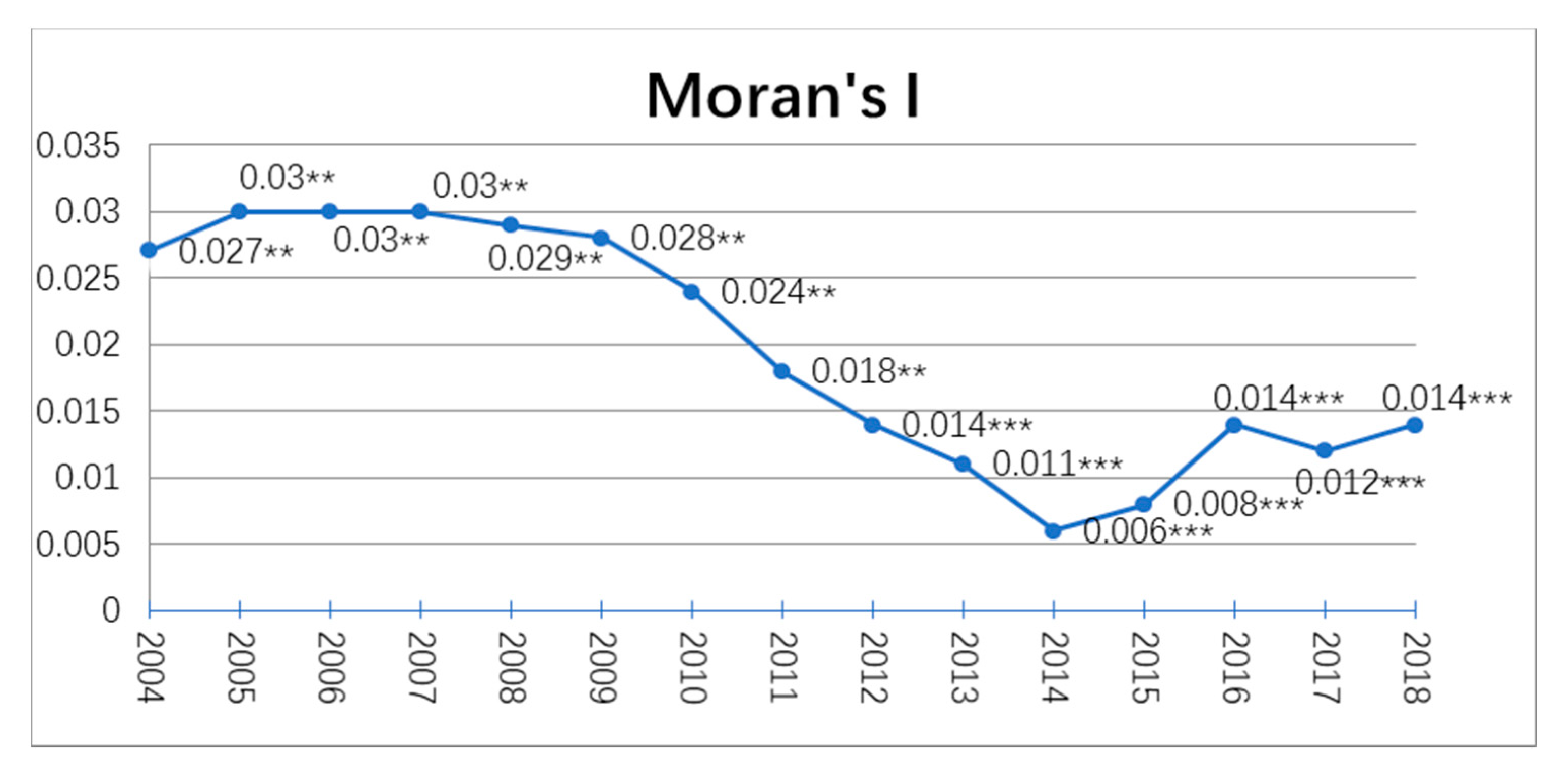
Figure 3 shows the results of the global Moran’s I index of lnec. The Moran’s I fluctuated from 0.006 to 0.03 at the confidence of 5% or 10% during the period of 2004–2018. It means the existence of a significant positive correlation with the spatial distribution. The dynamic changes of the index reflect the weakness or strengthens of the spatial agglomeration. From 2005 to 2014, the Moran’s I had a substantial decrease, but it gradually increased after 2014, except for a slight decline in 2017. Therefore, it is clear that the spatial autocorrelation became weaker gradually between 2005 and 2014, but it increased after 2014.
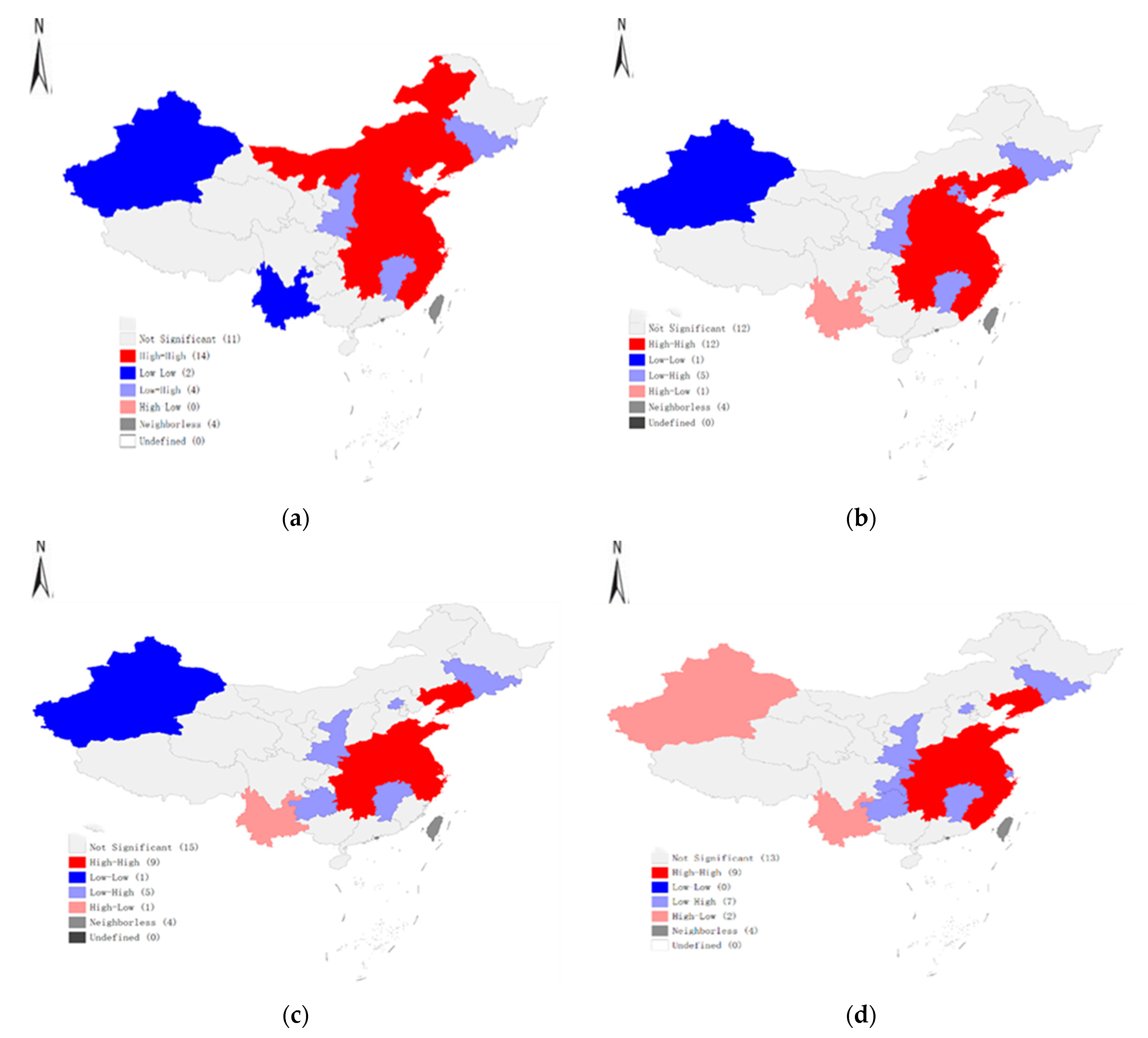
The results of global Moran’s I index mean that electricity consumption has a positive spatial correlation. However, it cannot reveal the local distribution of high-cluster areas or low-cluster areas. In view of this, this study calculated the local Moran’s I index of electricity consumption in 2004, 2008, 2012 and 2018 to further indicate whether there is a local spatial agglomeration phenomenon for electricity consumption. The results are shown in Figure 4.
As shown in Figure 4a, most provinces in 2004 fall into HH clusters, which are mainly concentrated in Beijing, Hebei, Inner Mongolia, Shandong, Jiangsu, Zhejiang, and Fujian, etc.; Xinjiang and Yunnan are the LL clusters; The LH clusters include Tianjin, Shaanxi, Jiangxi, and Jilin; The HL cluster is zero. Compared with 2004, Figure 4b shows some changes in 2008, namely, Beijing from HH to LH, Inner Mongolia from HH to no significance, Yunnan from LL to HL. Figure 4c shows that some changes between 2008 and 2012 are Hebei, Shanxi, and Fujian from HH to no significance, Tianjin from LH to no significance, and Guizhou from no significance to LH. Compared with 2012, Figure 4d indicates some changes, namely, Fujian from no significance to HH, Xinjiang from LL to HL, Shanghai from HH to LH, and Chongqing from no significance to LH. Figure 4 has also shown that the spatial agglomeration of electricity consumption has been transformed and differentiated over time. HH clusters changed from 14 provinces in 2004 to 9 provinces in 2018, and LL clusters dropped from 2 provinces in 2004 to 0 in 2018. LH clusters changed from 4 provinces in 2004 to 7 provinces in 2018, and HL clusters rose from 0 in 2004 to 2 provinces in 2018. The results mean that the spatial agglomeration of electricity consumption in local regions is mainly HH clusters, and the HH clusters are gradually weakening between 2004 and 2018. The reasons for the transformation are manifold, one of which lies in the significant pressure on China’s resources and environment caused by the growing demand for electricity. Policymakers have put more effort into energy conservation and emission reduction. The outline of the China’s 13th Five-Year (2016–2020) Plan for Economic and Social Development clearly states that the energy consumption per unit of GDP is to be reduced by 15% and CO2 emissions per unit of GDP by 18% during this plan period. In contrast, the promotion of clean energy and energy-saving technologies is also an important reason for the transformation.
4.3. Results of Spatial Model
The estimation results of all models are presented in Table 5. In order to choose the optimal model, we need to test the null hypothesis:: , and . The former tests whether SDM can be simplified to SAR, and the latter tests whether SDM can be reduced to SEM. If the null hypothesis is rejected, SDM is more suitable [57]. This paper adopts the Wald test and LR test to judge whether the SDM can be simplified to the SAR and SEM [58]. The Wald-lag and LR-lag statistics are 21.17 and 20.64, respectively, so SDM is more proper than SAR; the Wald-err and LR-err statistics are 18.93 and 38.93, respectively, therefore, SDM is superior to SEM. The test results are significant at 1% confidence interval, and thus the SDM is the optimal model. According to the result of the Hausman test (14.61, p > 0.10), the null hypothesis (random effects model) is accepted. Therefore, the random effect is more suitable for the model in this study.
LeSage and Pace [58] found that the spatial spillover effect is not simply represented by the regression coefficient of the spatial lag term, and the application of partial differential methods can correctly measure the direct, indirect (spatial spillover) and total effects of the explanatory variables. By rewriting SDM as:
The above equation can be transformed into:
In this coefficient matrix, the average of the diagonal elements () represents the direct effect of the kth explanatory variable, while the average value of the total row of non-diagonal elements () indicates the indirect effect of the kth explanatory variable, i.e., the spatial spillover effect. The total effect of the explanatory variable is the aggregate of all direct and indirect effects. The results from the direct, indirect, and total effects of the random effect SDM model are presented in Table 6.
According to Table 6, the direct effect of lnfde is significant and positive at the 1% level, namely, financial development promotes electricity consumption. Specifically, the empirical results show that a 1% increase in financial development will lead to a corresponding increase of 0.089% in electricity consumption if all other factors remain unchanged. Sadorsky [59] revealed that financial development can increase energy consumption through consumer effect, business effect and wealth effect. This is debatable because financial development induces investment in innovations in the areas of energy conservation and energy efficiency to trigger a reversal effect on energy consumption [23]. Our study shows that the positive effect of financial development on electricity consumption can offset the impact of technological change on electricity consumption, and the result is supported by [20,59]. The direct effect of lntro is significant and negative at 5% level. Consequently, a 1% rise in trade openness decreases electricity consumption by 0.051%. The common belief about trade openness is that export leads to an increase of economic output and therefore amplifies electricity consumption [7,27]. However, a different viewpoint may be true. Trade openness may improve electricity use efficiency by introducing advanced technologies and high-tech industry, and the access to reduced electricity-intensity products is easier. Further, the promotion of clean energy has boosted the demand for environmentally friendly products, thereby reducing the demand for electricity. Sbia et al. [8] revealed that a 0.363% energy demand is declined by 1% increase in trade openness. Our result is consistent with other scholars such as Refs. [8,24] among others.
With respect to the spatial effects of financial development and trade openness on electricity consumption, the indirect effects reflect the spatial impacts of the explanatory variables on the dependent variable. The indirect effect of lnfde is weakly significant and negative at 10% level, namely, a 1% rise in financial development reduces electricity consumption of neighboring regions by 0.051%. The result means that financial development accelerates technology sharing with surrounding provinces and reduces electricity consumption in neighboring provinces by improving the efficiency of electricity use. The indirect effect of lntro is not significant. One possible explanation is that the technology spillover effect of trade openness is relatively weak, and it is difficult to reduce electricity consumption in the surrounding provinces.
For the control variables, the direct effects of lnpgdp and lnind are significant and positive at the 1% and 5% levels, respectively, which means that economic growth and industrialization promote electricity consumption during the research period. The direct effect of lnfai is significant and negative at the 5% level, which indicates that there is a significant negative correlation between fixed asset investment and electricity consumption. The direct effects of lnfdi and lnurb are not significant, which means that foreign direct investment and urbanization have no impact on the electricity consumption. According to the results of spillover effect, the indirect effects of lnpgdp, lnfai and lnurb are significantly positive at 5% levels, respectively, which means that economic growth, fixed asset investment and urbanization lead to an improvement in electricity consumption of surrounding regions. The indirect effect of lnind is significant and negative at 1% level, which means that industrialization can result in a decline in electricity consumption of neighboring provinces. The indirect effect of lnfdi is not significant, indicating that foreign direct investment has no impact on electricity consumption of other regions.
4.4. PVAR Estimation Results
4.4.1. PVAR Lag Selection
The estimation quality of the panel VAR model depends on the selection of the optimal lag order. For this reason, Andrews and Lu [60] suggested consistent moment and model selection criteria for GMM models, which are based on Hansen’s J statistic of over-identifying restrictions. The criteria include Akaike information criterion (AIC), Bayesian information criterion (BIC) and Hannan Quine information criterion (HQIC). Table 7 presents the results based on the model selection criteria. According to the smallest MBIC and MQIC, this study selects the first-order panel VAR model.
4.4.2. Stability of the PVAR Model
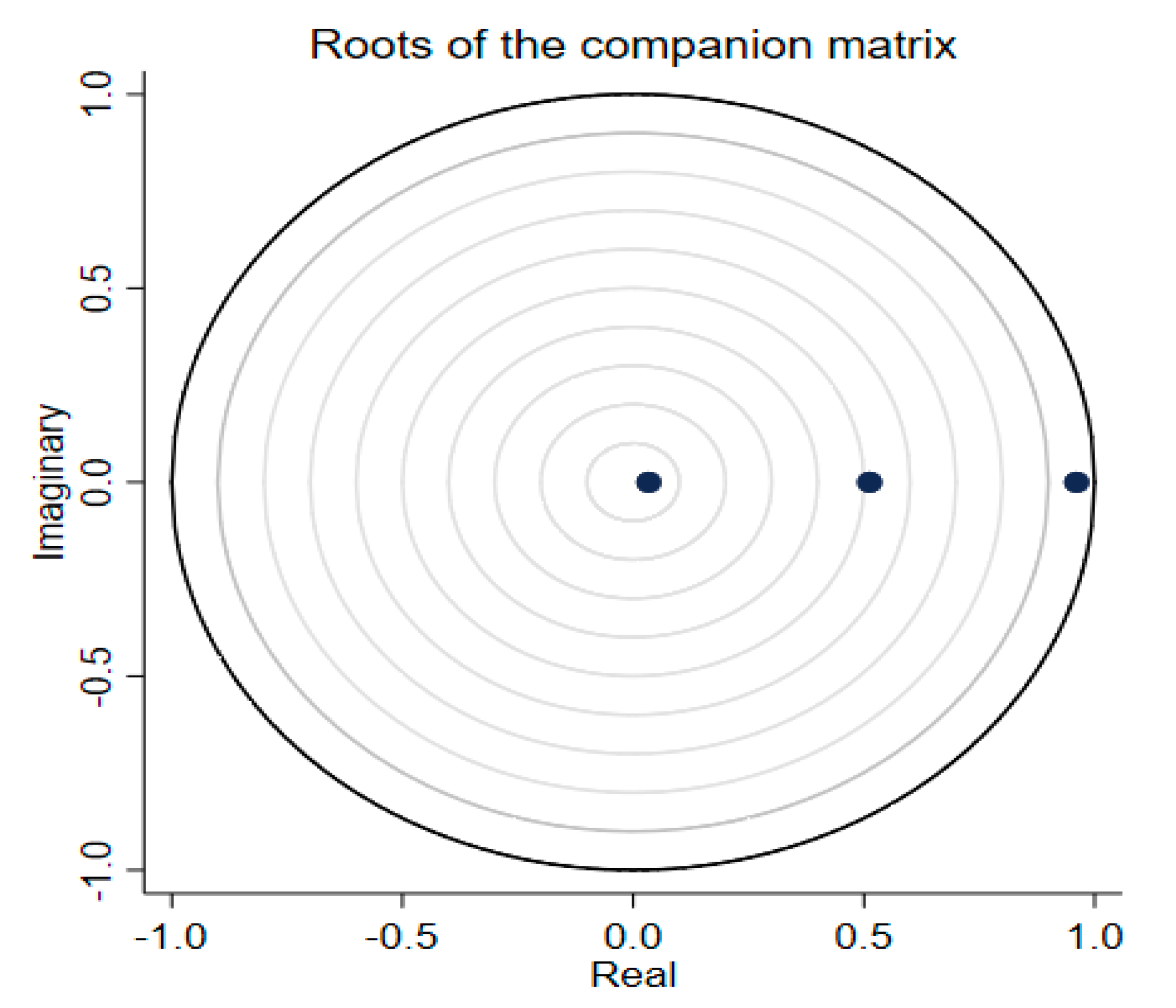
Checking the stability conditions is essential when estimating the PVAR model. Whether the PVAR is stable depends on the modulus of each eigenvalue of the estimation model. If each modulus in the companion matrix is strictly less than one, the PVAR model is stable [54]. Figure 5 confirms that the estimated PVAR model satisfies the stability condition.
4.4.3. Granger Causality Test
Because all variables in the PVAR model are assumed to be endogenous, we use Granger causality test to check for the validity of this condition. The results shown in Table 8 confirm that lnec, lnfde and lntro have a bidirectional causal relationship. The findings indicate that all variables in the PVAR model should be regarded as endogenous variables.
4.4.4. Impulse Response Function (IRF)
The IRF illustrates the reaction of an endogenous variable to one standard deviation shock of another endogenous variable. We calculate the orthogonalized IRF based on Cholesky decomposition, and the confidence interval is computed by using Gaussian approximation based on Monte Carlo 200 draws.
We start with the relationship between electricity consumption and financial development. Figure 6 shows that electricity consumption exhibits a positive response to a standard deviation shock to financial development from period 0 to period 10. The maximum positive impact occurs in the fourth period and then decreases slowly. This result reveals that financial development has a long-term promoting effect on electricity consumption. Next, we focus on the relationship between electricity consumption and trade openness. Figure 6 depicts that the graph is below the zero line, which means that a standard deviation shock to trade openness leads to a decrease in electricity consumption from period 0 to period 10. The maximum negative impact occurs in the first period and then increases gradually. This result reveals that trade openness has a long-term inhibiting effect on electricity consumption, but the inhibiting effect is gradually diminishing.
5. Conclusions and Policy Implications
In this study, we empirically analyze the direction and degree of the impact of financial development and trade openness on electricity consumption with China’s 2004–2018 provincial panel data using spatial econometric approaches and PVAR model. The following conclusions are drawn: First, China’s electricity consumption has a positive spatial correlation, and it shows a trend of agglomeration in spatial distribution. The spatial agglomeration of electricity consumption in local regions is mainly HH clusters, but over time, the HH clusters are gradually weakening. Second, according to the results of SDM with the geographic distance weight matrix, financial development is found to significantly increase electricity consumption within a province, and a 1% increase in financial development will lead to a corresponding increase of 0.089% in electricity consumption. This spatial spillover effect of financial development on electricity consumption is significantly negative, and a 1% rise in financial development reduces electricity consumption of neighboring regions by 0.051%. Third, the direct effect of trade openness on electricity consumption is significantly negative, with a 1% increase in trade openness decreasing electricity consumption by 0.051%, while the indirect effect of trade openness is not significant. Finally, regarding the impulse response results, our empirical findings show that the response of electricity consumption to one standard shock on financial development displays a positive sign, and the maximum positive impact occurs in the fourth period and then decreases slowly. The electricity consumption response to one standard deviation shock on trade openness shows a negative impact, and the maximum negative impact occurs in the first period and then increases gradually.
The findings of this paper provide valuable policy implications. First, policy makers should adjust and optimize the spatial correlation structure of electricity consumption and improve the regional allocation efficiency of electricity consumption. Second, financial development should be used as a policy tool to reduce electricity consumption. By accelerating green financial innovation, the financial sector is directed to sanction loans to those companies or industries that use advanced energy-efficient technologies in their production processes and who are environmentally friendly. Third, it should improve the structure of foreign trade, expand green trade, increase the proportion of energy-efficient import and export goods, and actively connect with the international frontier to learn and absorb advanced energy-saving technologies.
Author Contributions
Conceptualization, R.D. and P.G.; methodology, R.D.; software, P.G.; formal analysis, R.D.; resources, R.D.; data curation, P.G.; writing—original draft preparation, R.D.; writing—review and editing, R.D.; supervision, P.G.; project administration, R.D.; funding acquisition, R.D. All authors have read and agreed to the published version of the manuscript.
Funding
This research was funded by the National Social Science Fund of China, grant number 16BJY087.
Institutional Review Board Statement
Not applicable.
Informed Consent Statement
Not applicable.
Data Availability Statement
Not applicable.
Conflicts of Interest
The authors declare no conflict of interest.
Abbreviations
| PVAR | Panel vector autoregression |
| WTO | World Trade Organization |
| ARDL | Autoregressive distributed lag |
| VECM | Vector error correction method |
| GMM | Generalized method of moments |
| AIC | Akaike information criterion |
| HQIC | Hannan Quine information criterion |
| LLC | Levin-Lin-Chu |
| IPS | Im-Pesaran-Shin |
| REC | Residential electricity consumption |
| IEC | Industrial electricity consumption |
| SAR | Spatial autoregressive model |
| SEM | Spatial error model |
| SDM | Spatial Durbin model |
| BIC | Bayesian information criterion |
| IRF | Impulse response function |
| HT | Harris-Tzavalis |
References
- IEA. World Energy Outlook 2019; International Energy Agency: Paris, France, 2019; Available online: https://www.iea.org/reports/world-energy-outlook-2019 (accessed on 14 August 2021).
- Lin, B.; Li, Z. Is more use of electricity leading to less carbon emission growth? An analysis with a panel threshold model. Energy Policy 2020, 137, 111121. [Google Scholar] [CrossRef]
- IEA. Data-CO2 Emissions; International Energy Agency: Paris, France, 2021; Available online: https://www.iea.org/data-and-statistics (accessed on 7 August 2021).
- Zhou, G.; Chung, W.; Zhang, Y. Measuring energy efficiency performance of China’s transport sector: A data envelopment analysis approach. Expert Syst. Appl. 2014, 41, 709–722. [Google Scholar] [CrossRef]
- Sadorsky, P. The impact of financial development on energy consumption in emerging economies. Energy Policy 2010, 38, 2528–2535. [Google Scholar] [CrossRef]
- Liu, S.; Li, H. Does Financial Development Increase Urban Electricity Consumption? Evidence from Spatial and Heterogeneity Analysis. Sustainability 2020, 12, 7011. [Google Scholar] [CrossRef]
- Gregori, T.; Tiwari, A.K. Do urbanization, income, and trade affect electricity consumption across Chinese provinces? Energy Economics 2020, 89, 104800. [Google Scholar] [CrossRef]
- Sbia, R.; Shahbaz, M.; Hamdi, H. A contribution of foreign direct investment, clean energy, trade openness, carbon emissions and economic growth to energy demand in UAE. Econ. Model. 2014, 36, 191–197. [Google Scholar] [CrossRef] [Green Version]
- An, H.; Xu, J.; Ma, X. Does technological progress and industrial structure reduce electricity consumption? Evidence from spatial and heterogeneity analysis. Struct. Chang. Econ. Dyn. 2020, 52, 206–220. [Google Scholar] [CrossRef]
- Sadorsky, P. Information communication technology and electricity consumption in emerging economies. Energy Policy 2012, 48, 130–136. [Google Scholar] [CrossRef]
- Shahbaz, M.; Feridun, M. Electricity consumption and economic growth empirical evidence from Pakistan. Qual. Quant. 2012, 46, 1583–1599. [Google Scholar] [CrossRef]
- Salahuddin, M.; Alam, K. Internet usage, electricity consumption and economic growth in Australia: Time series evidence. Telemat. Inform. 2015, 32, 862–878. [Google Scholar]
- Al-Bajjali, S.K.; Shamayleh, A.Y. Estimating the determinants of electricity consumption in Jordan. Energy 2018, 147, 1311–1320. [Google Scholar] [CrossRef]
- Kumari, A.; Sharma, A.K. Causal relationships among electricity consumption, foreign direct investment and economic growth in India. Electr. J. 2018, 31, 33–38. [Google Scholar] [CrossRef]
- Lin, B.; Wang, Y. Inconsistency of economic growth and electricity consumption in China: A panel VAR approach. J. Clean. Prod. 2019, 229, 144–156. [Google Scholar] [CrossRef]
- Taale, F.; Kyeremeh, C. Drivers of households’ electricity expenditure in Ghana. Energy Build. 2019, 205, 109546. [Google Scholar] [CrossRef]
- Benjamin, N.I.; Lin, B. Influencing factors on electricity demand in Chinese nonmetallic mineral products industry: A quantile perspective. J. Clean. Prod. 2019, 243, 118584. [Google Scholar] [CrossRef]
- Zhang, M.; Chen, Y.; Hu, W.; Deng, N.; He, W. Exploring the impact of temperature change on residential electricity consumption in China: The ‘crowding-out’ effect of income growth. Energy Build. 2021, 245, 111040. [Google Scholar] [CrossRef]
- Rafindadi, A.A.; Ozturk, I. Effects of financial development, economic growth and trade on electricity consumption: Evidence from post-Fukushima Japan. Renew. Sustain. Energy Rev. 2016, 54, 1073–1084. [Google Scholar] [CrossRef]
- Sbia, R.; Shahbaz, M.; Ozturk, I. Economic growth, financial development, urbanisation and electricity consumption nexus in UAE. Econ. Res.-Ekon. Istraživanja 2017, 30, 527–549. [Google Scholar] [CrossRef] [Green Version]
- Faisal, F.; Tursoy, T.; Berk, N. Linear and non-linear impact of Internet usage and financial deepening on electricity consumption for Turkey: Empirical evidence from asymmetric causality. Environ. Sci. Pollut. Res. Int. 2018, 25, 11536–11555. [Google Scholar] [CrossRef] [PubMed]
- Solarin, S.A.; Shahbaz, M.; Khan, H.N.; Razali, R.B. ICT, Financial Development, Economic Growth and Electricity Consumption: New Evidence from Malaysia. Glob. Bus. Rev. 2019, 22, 941–962. [Google Scholar] [CrossRef]
- Adom, P.K. Financial depth and electricity consumption in Africa: Does education matter? Empir. Econ. 2020, 1–55. [Google Scholar] [CrossRef]
- Lin, B.; Omoju, O.E.; Okonkwo, J.U. Factors influencing renewable electricity consumption in China. Renew. Sustain. Energy Rev. 2016, 55, 687–696. [Google Scholar] [CrossRef]
- Ohlan, R. The relationship between electricity consumption, trade openness and economic growth in India. OPEC Energy Rev. 2018, 42, 331–354. [Google Scholar] [CrossRef]
- Ghazouani, T.; Boukhatem, J.; Yan Sam, C. Causal interactions between trade openness, renewable electricity consumption, and economic growth in Asia-Pacific countries: Fresh evidence from a bootstrap ARDL approach. Renew. Sustain. Energy Rev. 2020, 133, 110094. [Google Scholar] [CrossRef]
- Sahoo, M.; Sethi, N. Does remittance inflow stimulate electricity consumption in India? An empirical insight. South Asian J. Bus. Stud. 2020. ahead-of-print. [Google Scholar] [CrossRef]
- Anselin, L.; Rey, S.J. Introduction to the Special Issue on Spatial Econometrics. Int. Reg. Sci. Rev. 1997, 20, 1–7. [Google Scholar] [CrossRef]
- Jiang, L.; Ji, M. China’s Energy Intensity, Determinants and Spatial Effects. Sustainability 2016, 8, 544. [Google Scholar] [CrossRef] [Green Version]
- Wu, H.; Xia, Y.; Yang, X.; Hao, Y.; Ren, S. Does environmental pollution promote China’s crime rate? A new perspective through government official corruption. Struct. Chang. Econ. Dyn. 2021, 57, 292–307. [Google Scholar] [CrossRef]
- Zhang, J.; Wang, L.; Wang, S. Financial development and economic growth: Recent evidence from China. J. Comp. Econ. 2012, 40, 393–412. [Google Scholar] [CrossRef]
- Hao, Y.; Wang, L.-O.; Lee, C.-C. Financial development, energy consumption and China’s economic growth: New evidence from provincial panel data. Int. Rev. Econ. Financ. 2020, 69, 1132–1151. [Google Scholar] [CrossRef]
- Yuxiang, K.; Chen, Z. Financial development and environmental performance: Evidence from China. Environ. Dev. Econ. 2010, 16, 93–111. [Google Scholar] [CrossRef]
- Pan, X.; Uddin, M.K.; Saima, U.; Jiao, Z.; Han, C. How do industrialization and trade openness influence energy intensity? Evidence from a path model in case of Bangladesh. Energy Policy 2019, 133, 110916. [Google Scholar] [CrossRef]
- Pan, X.; Uddin, M.K.; Han, C.; Pan, X. Dynamics of financial development, trade openness, technological innovation and energy intensity: Evidence from Bangladesh. Energy 2019, 171, 456–464. [Google Scholar] [CrossRef]
- Zhou, D.; Chen, B.; Li, J.; Jiang, Y.; Ding, X. China’s Economic Growth, Energy Efficiency, and Industrial Development: Nonlinear Effects on Carbon Dioxide Emissions. Discret. Dyn. Nat. Soc. 2021, 2021, 5547092. [Google Scholar] [CrossRef]
- Sarkodie, S.A.; Strezov, V. Effect of foreign direct investments, economic development and energy consumption on greenhouse gas emissions in developing countries. Sci. Total Environ. 2019, 646, 862–871. [Google Scholar] [CrossRef] [PubMed]
- Zhao, X.; Zhang, Y.; Li, Y. The spillovers of foreign direct investment and the convergence of energy intensity. J. Clean. Prod. 2019, 206, 611–621. [Google Scholar] [CrossRef]
- Guo, Z.; Chen, S.S.; Yao, S.; Mkumbo, A.C. Does Foreign Direct Investment Affect SO2 Emissions in the Yangtze River Delta? A Spatial Econometric Analysis. Chin. Geogr. Sci. 2021, 31, 400–412. [Google Scholar] [CrossRef]
- Yan, L.; Guan, Z.; Yang, X. Relationship between Fixed-Asset Investment and Environmental Quality Based on EKC. In LISS 2013; Springer: Berlin/Heidelberg, Germany, 2015. [Google Scholar] [CrossRef]
- Mamipour, S.; Beheshtipour, H.; Feshari, M.; Amiri, H. Factors influencing carbon dioxide emissions in Iran’s provinces with emphasis on spatial linkages. Environ. Sci. Pollut. Res. Int. 2019, 26, 18365–18378. [Google Scholar] [CrossRef]
- Lin, B.; Zhu, J. Energy and carbon intensity in China during the urbanization and industrialization process: A panel VAR approach. J. Clean. Prod. 2017, 168, 780–790. [Google Scholar] [CrossRef]
- Yang, Y.; Liu, J.; Lin, Y.; Li, Q. The impact of urbanization on China’s residential energy consumption. Struct. Chang. Econ. Dyn. 2019, 49, 170–182. [Google Scholar] [CrossRef]
- Rathnayaka, R.M.K.T.; Seneviratna, D.M.K.N.; Long, W. The dynamic relationship between energy consumption and economic growth in China. Energy Sources Part B Econ. Plan. Policy 2018, 13, 264–268. [Google Scholar] [CrossRef]
- Levin, A.; Lin, C.-F.; Chu, C.-S.J. Unit root tests in panel data: Asymptotic and finite-sample properties. J. Econom. 2002, 108, 1–24. [Google Scholar] [CrossRef]
- Harris, R.D.F.; Tzavalis, E. Inference for unit roots in dynamic panels where the time dimension is fixed. J. Econom. 1999, 91, 210–226. [Google Scholar] [CrossRef]
- Im, K.S.; Pesaran, M.H.; Shin, Y. Testing for unit roots in heterogeneous panels. Adv. Econom. 2003, 115, 53–75. [Google Scholar] [CrossRef]
- Engle, R.F.; Granger, C.W.J. Co-integration and error correction: Representation, estimation, and testing. Econometrica 1987, 55, 251–276. [Google Scholar] [CrossRef]
- Pedroni, P. Panel Cointegration: Asymptotic and Finite Sample Properties of Pooled Time Series Tests with an Application to the PPP Hypothesis. Econom. Theory 2004, 20, 597–625. [Google Scholar] [CrossRef] [Green Version]
- Anselin, L. Local Indicators of Spatial Association-LISA. Geogr. Anal. 1995, 27, 93–115. [Google Scholar] [CrossRef]
- Elhorst, J.P. Dynamic Spatial Panels: Models, Methods and Inferences. J. Geogr. Syst. 2012, 14, 5–28. [Google Scholar] [CrossRef]
- Holtz-Eakin, D.; Newey, W.; Rosen, H.S. Estimating Vector Autoregressions with Panel Data. Econometrica 1988, 56, 1371–1395. [Google Scholar] [CrossRef]
- Love, I.; Zicchino, L. Financial development and dynamic investment behavior: Evidence from panel VAR. Q. Rev. Econ. Financ. 2006, 46, 190–210. [Google Scholar] [CrossRef]
- Zouaoui, H.; Zoghlami, F. On the income diversification and bank market power nexus in the MENA countries: Evidence from a GMM panel-VAR approach. Res. Int. Bus. Financ. 2020, 52, 101186. [Google Scholar] [CrossRef]
- Antonakakis, N.; Chatziantoniou, I.; Filis, G. Energy consumption, CO 2 emissions, and economic growth: An ethical dilemma. Renew. Sustain. Energy Rev. 2017, 68, 808–824. [Google Scholar] [CrossRef] [Green Version]
- Charfeddine, L.; Kahia, M. Impact of renewable energy consumption and financial development on CO2 emissions and economic growth in the MENA region: A panel vector autoregressive (PVAR) analysis. Renew. Energy 2019, 139, 198–213. [Google Scholar] [CrossRef]
- Belotti, F.; Hughes, G. Spatial panel-data models using Stata. Stata J. 2017, 1, 139–180. [Google Scholar] [CrossRef] [Green Version]
- LeSage, J.; Pace, R.K. Introduction to Spatial Econometrics; CRC Press, Taylor & Francis Group: New York, NY, USA, 2009. [Google Scholar]
- Sadorsky, P. Financial development and energy consumption in Central and Eastern European frontier economies. Energy Policy 2011, 39, 999–1006. [Google Scholar] [CrossRef]
- Andrews, W.K.D.; Lu, B. Consistent model and moment selection procedures for GMM estimation with application to dynamic panel data models. J. Econom. 2001, 101, 123–164. [Google Scholar] [CrossRef]
Figure 1.
Spatial distribution of China’s provincial electricity consumption in 2018. Note: Electricity consumption is expressed in units of 100 million kWh. Data source: the National Bureau of Statistics of China.
Figure 1.
Spatial distribution of China’s provincial electricity consumption in 2018. Note: Electricity consumption is expressed in units of 100 million kWh. Data source: the National Bureau of Statistics of China.

Figure 2.
Financial development and trade openness in China, 1992–2018. Data source: the National Bureau of Statistics of China.
Figure 2.
Financial development and trade openness in China, 1992–2018. Data source: the National Bureau of Statistics of China.

Figure 3.
Global Moran’s I of electricity consumption. Note: **, *** significant at the 5%, 1% levels, respectively.
Figure 3.
Global Moran’s I of electricity consumption. Note: **, *** significant at the 5%, 1% levels, respectively.

Figure 4.
Local Moran map of electricity consumption. (a) 2004; (b) 2008; (c) 2012; (d) 2018.

Figure 5.
Graph of Eigenvalue within the Unit Circle.

Figure 6.
Graphs of orthogonalized IRF.

Table 2.
Descriptive statistics.
| Variables | Unit | Mean | Std. Dev | Min | Max |
|---|---|---|---|---|---|
| lnec | 108 kWh | 6.909 | 1.028 | 2.163 | 8.752 |
| lnfde | % | 4.733 | 0.527 | 0.129 | 6.542 |
| lntro | % | 2.882 | 0.982 | 0.523 | 5.148 |
| lnpgdp | Yuan | 10.350 | 0.689 | 8.370 | 11.851 |
| lnfdi | 108 Yuan | 4.993 | 1.807 | −0.059 | 7.722 |
| lnfai | % | 4.174 | 0.581 | −1.020 | 6.370 |
| lnind | % | 3.578 | 0.385 | 1.918 | 3.971 |
| lnurb | % | 3.893 | 0.316 | 2.766 | 4.495 |
Data source: the National Bureau of Statistics of China.
Table 3.
Results of panel unit root test.
| Var. | Level | First Difference | ||||
|---|---|---|---|---|---|---|
| LLC | HT | IPS | LLC | HT | IPS | |
| lnec | −8.543 *** | 0.919 | −5.184 *** | −10.897 *** | 0.290 *** | −4.864 *** |
| lnfde | 1.213 | 0.326 *** | 5.429 | −5.755 *** | −0.568 *** | −8.373 *** |
| lntro | −14.174 *** | 0.253 *** | −5.230 *** | −3.066 *** | −0.501 *** | −12.337 *** |
| lnpgdp | −11.838 *** | 0.923 | −7.596 *** | −3.356 *** | 0.430 *** | −3.071 *** |
| lnfdi | 0.356 | 0.750 | −4.790 *** | −2.935 *** | −0.080 *** | −8.305 *** |
| lnfai | −5.491 *** | 0.425 *** | −0.102 | −3.862 *** | −0.562 *** | −6.873 *** |
| lnind | 3.227 | 0.974 | 7.941 | −6.657 *** | 0.294 *** | −5.641 *** |
| lnurb | −0.177 | 0.585 *** | −10.303 *** | −4.761 *** | 0.003 *** | −15.183 *** |
Notes: *** denotes statistical significance at 1% confidence interval.
Table 4.
Pedroni test for cointegration relationship.
| Statistic | p-Value | |
|---|---|---|
| Modified Phillips–Perron t | 2.8138 | 0.0024 |
| Phillips–Perron t | 3.1052 | 0.0010 |
| Augmented Dickey–Fuller t | 2.5965 | 0.0047 |
H0: No cointegration. Ha: All panels are co-integrated.
Table 5.
Estimation results of spatial panel data model.
| OLS | SAR | SEM | SDM | |
|---|---|---|---|---|
| lnfde | 0.112 *** (3.93) | 0.066 ** (2.57) | 0.104 *** (3.83) | 0.093 *** (3.29) |
| lntro | −0.047 ** (−2.08) | −0.062 *** (−2.88) | −0.062 *** (−2.76) | −0.053 ** (−2.28) |
| lnpgdp | 0.648 *** (24.22) | 0.389 *** (7.53) | 0.639 *** (21.38) | 0.310 *** (4.44) |
| lnfdi | −0.020 (−1.64) | −0.008 (−0.69) | −0.011 (−0.95) | −0.014 (−1.18) |
| lnfai | −0.078 *** (−2.78) | −0.041 (−1.64) | −0.071 *** (−2.64) | −0.072 *** (−2.60) |
| lnind | 0.011 (0.20) | 0.001 (0.003) | −0.048 (−1.06) | 0.176 *** (2.56) |
| lnurb | 0.230 *** (3.24) | 0.143 ** (2.09) | 0.159 * (1.91) | 0.116 (1.27) |
| W*lnfde | −0.224 ** (−2.00) | |||
| W*lntro | 0.124 * (1.71) | |||
| W*lnpgdp | 0.085 (0.67) | |||
| W*lnfdi | −0.105 (−1.47) | |||
| W*lnfai | 0.304 *** (2.85) | |||
| W*lnind | −0.444 *** (−4.05) | |||
| W*lnurb | 0.251 (1.60) | |||
| or λ | 0.386 *** (5.28) | 0.398 *** (3.10) | 0.352 *** (2.66) | |
| 0.899 | 0.902 | 0.898 | 0.906 | |
| LogL | 207.227 | 199.073 | 218.090 | |
| Wald spatial lag | 21.17 *** | |||
| LR spatial lag | 20.64 *** | |||
| Wald spatial error | 18.93 *** | |||
| LR spatial error | 38.03 *** |
Notes: *, **, and *** denote statistical significance at the 10%, 5%, and 1% significance levels, and the value in brackets is t-statistics.
Table 6.
Direct, indirect, and total effects of SDM with spatial random effects.
| Independent Var. | Direct Effects | Indirect Effects | Total Effects |
|---|---|---|---|
| lnfde | 0.089 *** (3.10) | −0.301 * (−1.71) | −0.211 (−1.19) |
| lntro | −0.051 ** (−2.31) | 0.171 (1.53) | 0.120 (1.08) |
| lnpgdp | 0.322 *** (4.89) | 0.287 ** (2.28) | 0.609 *** (5.52) |
| lnfdi | −0.016 (−1.43) | −0.171 (−1.38) | −0.187 (−1.48) |
| lnfai | −0.065 ** (−2.39) | 0.432 ** (2.37) | 0.368 ** (2.00) |
| lnind | 0.163 ** (2.57) | −0.594 *** (−3.52) | −0.431 *** (−2.72) |
| lnurb | 0.121 (1.31) | 0.460 ** (1.98) | 0.580 *** (2.71) |
Note: Numbers in parentheses represent t-statistics. *, **, and *** indicate significance at the 10%, 5%, and 1% levels, respectively.
Table 7.
PVAR Lag Selection Criteria.
| Lag | CD | MBIC | MAIC | MQIC |
|---|---|---|---|---|
| 1 | 0.9999 | −84.8228 | 16.0647 | −24.2659 |
| 2 | 0.9998 | −54.1424 | 13.1159 | −13.7711 |
| 3 | 0.9999 | −37.0663 | −3.4372 | −16.8807 |
Note: CD, MBIC, MAIC and MQIC are the overall coefficient of determination based on consistent moment and model selection criteria (the BIC, AIC, and HQIC, respectively).
Table 8.
Granger causality tests.
| Model | Null Hypothesis | chi2 | p-Value |
|---|---|---|---|
| Model 1: | lnfde(excluded) does not granger cause lnec | 12.261 *** | 0.000 |
| lnec and lnfde | lnec(excluded) does not granger cause lnfde | 138.272 *** | 0.000 |
| Model 2: | lntro (excluded) does not Granger cause lnec | 22.490 *** | 0.000 |
| lnec and lntro | lnec(excluded) does not granger cause lntro | 15.653 *** | 0.000 |
| Model 3: | lntro(excluded) does not granger cause lnfde | 7.985 *** | 0.005 |
| lnfde and lntro | lnfde(excluded) does not granger cause lntro | 25.278 *** | 0.000 |
Note: The values in the table are the Chi-square and their corresponding p-values. The null hypothesis is that the excluded variable does not Granger cause the endogenous variable. *** indicates rejection of the null hypothesis at 1% significance level.
Publisher’s Note: MDPI stays neutral with regard to jurisdictional claims in published maps and institutional affiliations. |
© 2021 by the authors. Licensee MDPI, Basel, Switzerland. This article is an open access article distributed under the terms and conditions of the Creative Commons Attribution (CC BY) license (https://creativecommons.org/licenses/by/4.0/).
Share and Cite
MDPI and ACS Style
Duan, R.; Guo, P. Electricity Consumption in China: The Effects of Financial Development and Trade Openness. Sustainability 2021, 13, 10206. https://doi.org/10.3390/su131810206
AMA Style
Duan R, Guo P. Electricity Consumption in China: The Effects of Financial Development and Trade Openness. Sustainability. 2021; 13(18):10206. https://doi.org/10.3390/su131810206
Chicago/Turabian StyleDuan, Ruijun, and Peng Guo. 2021. "Electricity Consumption in China: The Effects of Financial Development and Trade Openness" Sustainability 13, no. 18: 10206. https://doi.org/10.3390/su131810206
Note that from the first issue of 2016, this journal uses article numbers instead of page numbers. See further details here.