
Energy Loss Impact in Electrical Smart Grid Systems in Australia


1
Entrepreneurship, Commercialisation & Innovation Centre, University of Adelaide, Adelaide, SA 5005, Australia
2
Faculty of the Professions, Adelaide Business School, University of Adelaide, Adelaide, SA 5005, Australia
*
Author to whom correspondence should be addressed.
Sustainability 2021, 13(13), 7221; https://doi.org/10.3390/su13137221
Submission received: 25 May 2021
/
Revised: 22 June 2021
/
Accepted: 22 June 2021
/
Published: 28 June 2021
(This article belongs to the Special Issue Applications of Complex System Approach in Project Management)
Abstract
:This research draws attention to the potential and contextual influences on energy loss in Australia’s electricity market and smart grid systems. It further examines barriers in the transition toward optimising the benefit opportunities between electricity demand and electricity supply. The main contribution of this study highlights the impact of individual end-users by controlling and automating individual home electricity profiles within the objective function set (AV) of optimum demand ranges. Three stages of analysis were accomplished to achieve this goal. Firstly, we focused on feasibility analysis using ‘weight of evidence’ (WOE) and ‘information value’ (IV) techniques to check sample data segmentation and possible variable reduction. Stage two of sensitivity analysis (SA) used a generalised reduced gradient algorithm (GRG) to detect and compare a nonlinear optimisation issue caused by end-user demand. Stage three of analysis used two methods adopted from the machine learning toolbox, piecewise linear distribution (PLD) and the empirical cumulative distribution function (ECDF), to test the normality of time series data and measure the discrepancy between them. It used PLD and ECDF to derive a nonparametric representation of the overall cumulative distribution function (CDF). These analytical methods were all found to be relevant and provided a clue to the sustainability approach. This study provides insights into the design of sustainable homes, which must go beyond the concept of increasing the capacity of renewable energy. In addition to this, this study examines the interplay between the variance estimation of the problematic levels and the perception of energy loss to introduce a novel realistic model of cost–benefit incentives. This optimisation goal contrasted with uncertainties that remain as to what constitutes the demand impact and individual house effects in diverse clustering patterns in a specific grid system. While ongoing effort is still needed to look for strategic solutions for this class of complex problems, this research shows significant contextual opportunities to manage the complexity of the problem according to the nature of the case, representing dense and significant changes in the situational complexity.
1. Introduction
Despite the significant progress in monitoring and control technology in recent years, the energy loss rates in the grid system remain alarmingly high, and advocates warn that the increase in the number of Australian Electricity Market Operators (AEMO) creates a need for new approaches to wind up the issue. Considering the fact that the energy loss is significant, the issue was put under revision, and it was declared that this issue should be reviewed as a new version of guidelines could be met.
The power of the incompetence of end-users in mitigating energy loss could be one of the most inscrutable phenomena of the modern demand-side management of electricity (DSM), but it certainly has an impact. At this point, the demand for electricity will play a crucial role in upcoming smart grids that aim to link end-users and energy consumption in more efficient and better-balanced electrical grid systems. The nonlinearity of human behaviours that cause peaks and troughs leads to an enlargement of the gap between the supply of and demand for electricity. ‘Peak and off-peak demand periods’ are overwhelming the electrical grid system and are only resolved by providing better management for the demand side of electricity [1,2,3,4,5,6]. However, although various perspectives have provided diverse insights into this area, further work is needed to provide a consistent and integrated view on how to proceed. The current aim is to discuss the demand-side parameters, keep them efficient by re-considering the energy loss in the grid system, and promote the smart energy behaviour that is currently lacking. A literature review for this paper was conducted to establish a clear view of the three main aims: first, to review the state-of-the-art nonlinear dynamic engagement of end-user behaviour in smart grid projects, from both a theoretical and an empirical perspective; second, to summarise the key findings concerning the reported enablers and barriers for engaging end-users in smart energy behaviour; and third, to provide recommendations or ‘success factors’ for end-user engagement and recognise the many key challenges remaining for future research and development in Australia.
2. DSM Impact Globally
There has been a growing body of literature on the roots of the malfunctions that cause losses in grid systems, particularly the role of DSM in developing economies [7,8,9,10,11,12,13,14,15,16,17,18,19,20,21,22,23,24,25,26] (see Table 1).
Greater complexity in electrical demand systems is twofold, with one rise due to increasing the demand capacity and the other displayed as a factor of increasing the number of subjective consumers over time. Most DSM studies, as well as the sample database in Table 1 gathered from the recent five years of research, cover more than twenty countries on five continents. While arguments on these types of DSM studies are explicitly based on efficiency to ensure further access to electricity for developing economies, two stand out as definitively falling into environmental and social impacts. On the other hand, some other studies displayed the barriers due to a lack of technological adoption. However, rarely does evidence in the literature focus on the authenticity of energy loss and its impact on deriving an overall decentralisation solution.
Electricity power supply and demand are discrepant spatiotemporal utilities. However, enabling decentralised energy system transformation premises is adding a possible impact and multiple measures fronting energy loss. This problem of demand volatility has been further increased due to the growing penetration of renewable energy sources as it lacks a clear economic incentive for stakeholders that eventually translates to financial pressure. This cost burden issue sheds light on the necessity of maintaining demand stability and supply security as one of the significant challenges in the future [19,27].
In addition to this, and when it comes to the human factor, some studies tend to deliver answers that are eventual and firm. Unfortunately, that is not often the case in complex systems such as DSM. Although most studies have cognition about energy loss regardless of different views, these definitions stop somewhere where we could not agree more. This fact complicates any effort to decide which solution is transitional, leading stakeholders to argue about what should and what should not count. We think this research area still shows signs of being neglected mainly in developing nations. Therefore, our research effort provides analytical interpretations that have taken into account this cavity by involving interplay evidence dominated by the authenticity of energy loss.
3. Network Impact in Australia
Australia’s electricity networks comprise over 860,000 km of distribution networks and over 50,000 km of transmission lines. These networks are managed and operated by 23 businesses to deliver over 252 terawatt-hours (TWh) of total electricity generated for approximately 20 million customers [28,29]. A significant factor causing an increase in energy productivity (gross domestic product/energy consumption) is attributed to the growth in energy use for electricity generation (see Figure 1). Thus, there is a meaningful future increase in electricity generation based on the electricity demand and, mostly, a rise in the generation mix of lower-efficiency coal rather than renewables.
Coal is the primary fuel used for electricity in Australia, a source that has declined compared with past decades, but which is currently returning to higher and continuing use.
While coal remained the primary fuel source to generate electricity in 2014–2015, it has more recently fallen to 63%, which is well below its fuel mix share of above 80% at the beginning of the century [29]. In 2014–2015, coal-fired generation increased in South Australia, Queensland, and Victoria, with black coal rising by 2% and brown coal by 11%. This growth followed five consecutive years of decline in brown coal-fired generation and seven years in black coal-fired generation. The higher prices of gas and decreased hydro generation due to a lack of water availability reflect the switch to coal. This likewise coincides with the removal of the carbon price [30]. Natural gas-fired generation represents 21% of total electricity generation in Australia.
Table 2 shows that renewable energy makes up approximately 14% of Australia’s total electricity generation. The lower water levels in hydro dams led to a decline in hydro generation of 27% in 2014–2015, causing a decrease in the renewable generation of 7%. Hydro continues to be the largest contributor to renewable energy, with a share of 39%. This share is, however, at its lowest since the drought of the mid-2000s. Wind sources have become the second highest renewable behind hydro with its 33% contribution of renewable electricity and 5% of total electricity generated in Australia. Solar generation has been noticeable, growing in scale to 23%, but only addresses 2% of total electricity generation in Australia. This capacity of solar is only limited to large-scale solar installations. However, rooftop solar PV installation is still assumed to be the most reliable source for total solar generation in Australia [30].
As described in Table 2, a high proportion of irregular output comes from wind generation and is used for thermal generators. This adds to the advantage of an increase in the overall capacity of the energy generation mix. It would also add a higher degree of intermittency for stakeholders in the overall electricity supply [31].
The increasing intermittency of generation causes increased volatility in wholesale electricity spot prices. This influence has been observed in South Australia recently [31]. Following the increased spot price volatility, it would also increase the risk level that mostly retailers and consumers will carry. One means by which the volatility of spot prices can be managed is by purchasing higher-cost hedge contracts. These costs affect consumers through higher retail prices, which are passed on by electricity retailers [32].
As such, a large-scale renewable energy target (LRET) increases complex integrations that influence the costs of wholesale electricity [31,33]. Increased consumption puts upward pressure on costs. LRET encourages renewable energy investment to suppress wholesale costs, but this could well cause generator retirements over time. Intermittent forms of renewable generation will lead to higher spot market volatility, increasing costs, and retailers’ risks. These impacts cause upward pressure on wholesale electricity costs, as summarised in Table 3.
4. Trading Impact
The supply of electricity in Australia has a massive economic benefit. The annual turnover was AUD 22 billion during the financial year 1997–1998, total asset worth was estimated at AUD 67 billion, and 33,099 people were employed in this sector. The generating capacity recorded for the Australian electricity industry was approximately 48,000 MW [34]. Total electricity consumption registered in 1997–1998 was approximately 161,762 GWh, and over 180,000 GWh was produced in the same year. There are some 8.5 million customers, of whom 85% are residential customers, responsible for the consumption of 30% of the total consumed electricity. The average residential consumption per customer was approximately 2500 kWh per year, referring to 1997–1998 [35]. However, currently, the average has escalated to 6500 KWh. A household fuel and power expenditure survey in 1998–1999 showed that 72% of this value was consumed for electricity [36,37,38].
The annual averages, which are usually quoted for the wholesale electricity market, were masked by the feature of volatility in prices. Notice that Victoria’s average daily prices on many occasions went above AUD 2300 per megawatt-hour at certain times in peak hours. During peak time intervals, trades of spot prices climbed to the NEM price cap of AUD 12,500 per megawatt-hour in mid-2010 (see Figure 2) [39]. Extreme price movements are one of the challenges facing wholesale electricity providers, and, for this reason, the wholesale providers use the financial market instruments to hedge against unexpected extreme trends (see Figure 3).
Ascending prices are stacked on bids for producing electricity received by AEMO for orders defined for each dispatch period. Generators are then progressively scheduled into the needed production to cover the epidemic demand. This procedure starts with the least costly generation option. Therefore, the cost of generating power increases and decreases in response to the demand for electricity affected by consumer behaviour.
The electricity delivered by networks is mostly traded on behalf of two wholesale electricity markets in Australia [39]. The first market is NEM administered by AEMO which operates in NSW, Queensland, the ACT, South Australia, Victoria, and Tasmania [28]. The second operating market is WEM administrated by IMO which operates the South West Interconnected System. The target of both markets has as their objective the supply of energy from generation stations to customers in the least costly and most efficient way.
The drivers for each augmentation to transmission and distribution networks shown in Figure 4 take into account the criteria of security, quality, reliability, and safety standards. The weighted average loss of electricity through transmission and distribution networks combined is estimated at 5800 GWh (20.8 PJ) and equal to 6.7% of total inputs. Some studies found 15% of losses in transmission lines are due to transformers, with conductors making up the remaining 85%. The Australian weighted average loss for distribution networks and out of the total input is approximately 5.4% (2008–2009 to 2010–2011) and is equal to 9300 GWh p.a., which equals 33.48 PJ. Losses for individual networks in distribution areas operated by different retailers range from 3.7% to 9.1% [28].
There are significant differences, certainly, between supply and demand for electricity, but they share something remarkable. Each has managed to construct its own one-sided microclimate, in which peak or off-peak would technically be the sources of energy loss. This is a very serious matter with tragic consequences that, by any means, distress operational symptoms, associated as part of the unfavourable overall spectacle.
Electricity can be identified as an equally uniform commodity that is ultimately difficult and hard to adjust to brand differentiation or products. Electricity cannot be dealt with as goods in itself but as an input to produce other services and goods that are consumed as a final product. Therefore, the demand is sensitive for what is derived and is not as price-sensitive. Of course, the problem is the apparent confusion amongst electricity marketing administrators about what could preserve the expected profit ‘electricity bidding and wholesale processes’ which constitute the behaviour of a nonlinear dynamic of electricity demand.
It is evident that there is a financial risk for the participants in the National Electricity Market (NEM). This risk is associated with the significant degree of spot price volatility in every trading period (half an hour), which needs to be managed. Currently, there are two options for financial contracts. First, hedge contracts (see Figure 4) lock the electricity pricing in at a firm price at a given time in the future to reduce the financial exposure and provide spot market stability [33]. The alternative to the ‘hedge contract’ is a typical agreement between customers and generators to reduce the risk of spot prices. Hedge contracts may be arranged under long-term or short-term contracts and are not regulated according to rules but to help operate the market and AEMO’s administration independently. Unfortunately, the outcome of these contracts only provides more time rather than balancing between the supply and demand of electricity. These contracts arrange the price of electricity traded through the pool, known as the ‘agreed price’ or ‘strike price’ [33]. The advantage of these contracts is that they reduce the risk of the spot price’s potential volatility but cannot avoid its influence. The strike price operates when generators pay customers the gap when the spot price is above the strike price. Consequently, customers (retailers) will pay generators the difference between the strike price and spot price when the spot price is found to be below the strike price. Apparently, the risk of the spot price exists due to demand fluctuation.
5. Cost and Price Impacts
Electricity prices throughout the 1990s were curbed against price inflation features. Recent years have seen a notable increase in Australia’s electricity prices following pressure to increase the feature of ‘consumer price inflation’ [41]. In light of the range of factors influencing increased electricity prices, they are apparently moving upon cost-based pricing concepts, including increased investment to expand/replace ageing infrastructure which leads to increases in input costs; the direct impact of utility prices incurred at peak times added to aggregate inflation, and firms lodge higher input costs resulting from rising electricity prices and for other services.
The concentricity of ‘regulators’ models’ is based on how to provide revenues in advance for a pre-specified period to recover the expected efficiency costs incurred while delivering the regulated goods of ‘electricity’. As such, the expected revenues must be in line with the structured nature of any competitive market. Economic regulation takes various forms, each of which has implications for how a regulated firm’s costs influence the allowed revenues out of prices it charges to customers. The rationale for electricity cost price regulation is rooted in treating ‘market failures’. On the other hand, Australian political preferences and institutional frameworks have devolved enormous regulatory power to independent regulatory agencies nominated based on criteria of high quality, as presented in Figure 5 above. Australia has also been supporting its use of regulation by contracts with no dependency on outsourcing of regulatory functions to other parties [42].
Figure 6 refers to the governing structure designed toward electricity demand–supply relationships in Australia defined as the Australian Energy Regulator (AER). This independent body has the authority to play the role of electricity regulator in the NEM, originated by the Australian Competition and Consumer Commission (ACCC) that came into force in 2010 via the Competition and Consumer Act 2010. An associated requirement with this regulation is the Australian Energy Market Commission (AEMC) response for energy market rule settings. The AEMC is available under the Standard Council of Energy and Resources (SCER) controlled by, and which answers directly to, the peak intergovernmental forum in Australia known as the Council of Australian Government (COAG). Figure 6 above illustrates the existing top-down structure and relationships of the COAG, SCER, AEMC, AEMO, and AER toward suppliers, retailers, and electricity [43].
The AER has multiple functions to maintain monitoring of the market activities and behaviour within the NEM framework and keep up to date with market conditions to meet compliance issues. The AER is also responsible for defining the significant variations between actual and forecast prices of electricity and for tracing the contract markets’ movements, together with the analysis of rebidding behaviour and spot market outcomes [44]. The AER plays the role of setting the network charge components of retail electricity prices. The estimation must cover the amount of revenue wished for to cover a network provider’s costs over a five-year regulatory control period in addition to operation and maintenance (O&M), tax liabilities, asset depreciation costs, and return on capital.
Selling electricity has a ‘lumpy nature’ of investments. This means each particular year has different annual allowed revenues (AAR) represented by the sum of the right-side building blocks in Figure 7 (Depreciation, Return, and OPEX) [45]. OPEX is sometimes included in CAPEX as ‘pay-as-you-go’ items that are efficiently undertaken by OPEX in a particular year (see Figure 7 and Figure 8). A cumulative historical investment collected for a firm can be exhibited through the net cash recovered from regulatory depreciation, which in many cases requires a ‘coiling’ via the regulatory asset base (RAB) to assume the right deterministic model for CAPEX and returns on capital.
The tariff structures of Australia’s electricity distribution network are increasingly outdated and unfair. Current tariff structures do not reflect either the drivers of network costs or various customer uses of the network. Realistically, consumer load profile diversity will continue to grow as the use of solar panels, energy efficiency, and air conditioning increases [44]. The value must drive the focus on energy growth from the angle of distributor energy resources (DER) and the energy storage they create, instead of transferring costs among stakeholders (users). It would need to review electricity network tariffs that are in place today. The use of tariff options is effective in ‘flattening’ the load curve and reducing the peak demand to reduce losses at peak times. The role of tariffs bound to demand loads grows. Tariffs attempt to provide greater utilisation of the network capacity towards reducing the effects of increasing losses.
In the basic form, interval smart meters facilitate a greater range of implementing tariff options for ‘distributor network service providers’ (DNSP). Additionally, interval smart meters are used to gather information on the perception of consumer consumption patterns for improvements in network management. Multiple tariffs were deployed and data were collected from interval meters to deliver more cost-reflective tariffs for household consumption during peak and load baseline times, i.e., time of use tariffs (TOU), and capacity- and demand-based tariffs [50]. The eventual influence of tariffs is mainly designed to modify the load shape to optimise network capacity. As illustrated in Figure 9, the influence of tariffs found in the route of residential peak demand during the day has been practically changed [51]. The highest 5% of the demand has been trimmed and shifted from peak times to other off-peak times, which are good outcomes [28].
In the basic form, interval smart meters facilitate a greater range of implementing tariff options for ‘Distributor Network Service Providers’ (DNSP). Additionally, interval smart meters are used to gather information on the perception of consumer consumption patterns for improvements in network management. Multiple tariffs were deployed and data collected from interval meters to deliver more cost-reflective tariffs for household consumption during peak and load baseline times, i.e. Time Of Using Tariffs (TOU), and Capacity and demand based tariffs [50]. The eventual influence of tariffs is mainly designed to modify the load shape to optimise network capacity. As illustrated in Figure 9, the influence of tariffs found in the route of residential peak demand during the day has been practically changed [51]. The highest 5% of the demand has been trimmed and shifted from peak times to other off-peak times, which are good outcomes [28].
In real terms, prices for electricity increased on average 72% within a period of one decade to June 2013. Disregarding the slightly improvement of peak load shifting; It is seen practically; tariffs did not lead to decreasing the load on the peak times. This also concurrent with the increase for electricity demand has been 107% in Sydney, 73% in Brisbane, 41% in Adelaide and 30% in Perth. The contradiction found here is that the economic justification through the introduction of the interval meters uses tariff cost reflectively, to improve the use of network utilisation and reduce network demand. The side effect of this process of using meters and available tariff options obviously increases the use of the grid networks’ total capacity, expanding from less to more network energy loss [28]. Thereby, tariffs, tasked with improving network usage and decreasing the peak demand effect, have not yet helped flatten the demand load and decrease the peak effect (see Figure 10).
It is irrefutable that RAB delivers cost-plus regulating features that are achieved from the retrospective records of cost accounting values. Regulatory regimes have different asset records, different planned values subsequent to asset values and different accounting practices. These features need different mechanisms for adjustments, disallowances and time lags, and also the practising of particularly highlighted rules that require different re-evaluation to assets under construction and ongoing assets book entry. Therefore, there is no ideal link between RAB and the centralised asset values (electricity generation, transmission, and distribution).
6. Energy-Loss Impact
Demand loads and generators for transmission and distribution are unequal, making the output of the transmission networks uneven as the bulk supplies to the distribution networks are connected to it [52]. The average loss occurring in distribution and transmission networks is about 6% and interconnector loss of less than 1%, as combined average loss is estimated to make the total loss in Australian electricity networks 7%, proportional to the nature of daily energy demand and energy forecast horizon (see Figure 11). In general, the energy loss in grid systems is still under investigation because energy loss resulting from unfixed and differently integrated factors make it hard to consider the loss fixedly.
Some regulation Impact Statements had been formed to define efficient ways for network expansion. Those statements highlight that there is a lack of reliable and publicly available information on losses and trends occurring through transmission and distribution networks. Besides, network businesses and specialised agencies are not tasked with consistently and systematically gathering and reporting losses in information off the grid. This lack of transparency could be addressed as an addition to the reporting requirements through the electricity regulatory frameworks [52].
The Commonwealth made one meaningful attempt to foster greater understanding and support for measuring the implementation of distribution and transmission networks. In a frequent refrain, programmes such as ‘Energy Efficiency Opportunities’ (EEO) are assumed to achieve ‘cost-effective energy efficiency’. This programme divides energy usage into two segments: energy used through business operations (Type 1) and energy used through transmission and distribution (Type 2) [53]. Objectives are still targeted in accordance with the improvement options of Types 1 and 2 to reduce the losses from either electricity transmission and distribution or business operation by electricity providers. In 2012, the Australian Energy Market Commission released a report indicating that no benefits had been delivered from Type 2 energy loss saving projects.
Moreover, a recent analysis saw no other achievement in meeting the Commonwealth’s policy objectives. It seems that no energy efficiency improvements are expected to be achieved. By increasing the electricity costs for consumers, there is an additional administrative burden on electricity businesses.
Although the ‘Grid Australia’ report predicts Australia’s most efficient electricity grid yet, notwithstanding the shortcomings highlighted above, Types 1 and 2 for losses reduction (energy used via transmission and distribution) are still valid. Both EEO and the NEM take account of the current regulatory obligation of the NEM [53]. The NEM primarily focused on efficiency, which creates a conflict between the objectives that have no risks supported by the programmes of EEO.
Realistically, the electricity baseload requirements will be mainly provided by technologies based on fossil fuels [1]. Objectives are still targeted in accordance with the improvement options of Types 1 and 2 to reduce the losses from either electricity transmission and distribution or from business operation by electricity providers. As regards ‘Climate Works’, the improvement in each single percentage point (1%) in the grid performance is assumed to cost AUD 1.2 billion [53]. Further, Grid Australia found that a decrease in energy loss from 8% to 6.5% needs to improve 20% of the energy transfer from generators to end-users (transmission and distribution systems). Therefore, how much would that probably cost?
7. Methods
Following the guideline in demand-side management settings allows us to shed more light by testing data based on feasibility during stage one and sensitivity analysis in stage two, and by demonstrating findings validation in stage three. These analytical stages should help determine which guidelines of energy loss domains are implemented more effectively than others in electricity demand practice. We decided to adopt these methods because we believe that end-user behaviour could be understood as opportunistic states to assess the extent of individual commitment ‘to what the electrical grid is dealing with’. A sudden conflict or violence in such a complex system is likely to occur and possibly remain dissimilar within various clustering scales. This tension status can primarily be derived by measuring the level of conflict between the feasibility and the adopted study’s validity [54]. It refers to a mutually dependent relationship between these two different forms of the meaning to cause as either elevating or degrading the systems’ quality indicator. Thus, it possibly has negative (undermine) or positive (overestimate) tension between the concepts of feasibility and validity.
Nevertheless, perfect measures are not usually achieved in a study and not under circumstances where the scores are too low. Thus, the case would concern how much the procedure or instrument used to generate scores suits the tested sample. It is essential to ensure whether the sample has (or to see if it has not) attained the required fit for a proposed, tested module. The relevance of whether the data collected are feasible and valid relies on measuring what they are supposed to measure. The research’s validity implies the degree of confidence that can be inferred from the meaning attached to the collected data. Thus, no study is valid unless it reaches the level of feasibility. However, feasibility does not mean the study is valid because it accidentally does not measure what it is expected to measure. Our intention in this study is to conduct minimal measurement errors by considering the above factors that will be applied suitably to signify the chance of feasibility and validity. Thus, there is a need to demonstrate this study and its purpose, depicted in Figure 12 of the analysis module. We will limit ourselves to testing feasibility, sensitivity, and validity. We will revisit the results of sensitivity analysis, and, in addition, we will compare the optimisation results to a number of alternative validity tests. Both the power and the simulation optimisation of the sample data will be tested, all available in this manuscript.
7.1. Stage 1 Data Feasibility: (WOE) and (IV)
A wide range of studies address the aspect of feasibility from different perspectives and through various measures [54]. However, this study’s feasibility aims to measure whether a specific optimisation task of demand-side management is capable of being carried out when applied at several different individual houses. It is essential to decide whether this research’s feasibility is affordable for the designed objectives. Thus, stage one is attributed to testing the practicality of using time series data for the proposed optimisation method, described in stage two.
The feasibility stage focuses on using ‘weight of evidence’ (WOE) and ‘information value’ (IV) tools to check the sample data segmentation and possible variables reduction. The outcomes’ result of WOE and IV sheds light on the magnitude of the occurrence of peak (u) and off-peak (l) demands of bad events and the magnitude of non-occurrence of an average (AV) demand of good events, where this analysis is highly limited to predicting binary outcomes of events and no events.
A set of two formulated WOE and IV trials are proposed to increase the chance of discovering any imputation for missing values for greatly speeding up the step of selecting and reducing invalid variables. WOE and IV simulation will efficiently evaluate the predictive power of variables from three perspectives: continuous, ordinal, and categorical variables. This study only focuses on ‘continuous variables’ as we intend to measure tiers of an infinite number of possible values of peak, average, and off-peak demands numerically. To conclude, WOE and IV are used in stage one to select, reduce, analyse, and evaluate the binary outcomes of continuous dependent variables (interval electricity demand) for individual end-users. WOE and IV provide meaningful insights about the set of data we are using in this study, within a five-point scale of non-useful for prediction, weak, medium, strong, or suspicious predictive power.
WOE1 and WOE2:
where
- : The number of negative data items;
- : The number of positive data items;
- N: Total number of values;
- i: Demand value;
- A: Total number of end-users;
- WOE1: Original weight of evidence;
- WOE2: Alternative weight of evidence;
- IV1: Original information value;
- IV2: Alternative information value;
Conceptually, there is a strength associated between the study feasibility and validity at the level that makes us unable to separate them from each other. This unavoidable process of overlapping between the concept of feasibility and validity becomes exceedingly complex when the scales of validity increase (sample size, agents’ dissimilarity) and feasibility decreases (relevant factors such as technical, economic, and legal). Contrary to this, easily measurable indicators may ignore the complexity of energy loss, making the indicator more challenging to measure fact-based issues in depth, thus minimising the study’s feasibility. Although no specific rules provide an absolute balance between the validity and feasibility concepts, both must be bound to a great agreement to provide the appropriate tension needed for the systems’ quality indicator.
7.2. Stage 2 Optimisation Simulation: (SA)
In stage two, we used sensitivity analysis (SA) to investigate household systems’ optimisation in two scenarios: fossil fuel power supplied from the grid against mixed demand supplied from fossil fuel power generation and renewable power installed at individual houses [55]. We propose three main patterns of electricity consumption: (l), (u), and (AV), against three main parameters of electricity demand: (CL), (GL), and (GG). Thus, the modelling demand of electricity for individual end-users is mainly established to recognise the role of installed solar power generation systems (GG) as an ‘asset unit approach’ at homes to balance the grid system demand (CL and GL). The purpose of simulation analysis is to predict the extent of (GG) at homes in the mitigation of the effect of (l) and (u) and enhance the effect of (AV). Therefore, built-in tools such as GRG Nonlinear, LP/Quadratic, SOCP Barrier, Evolutionary, and Intemodelal in (SA) software are used in modelling the electricity demand profiles of end-users collected from AEMO data libraries. In other words, deployment time series data of home smart meters were targeted in this study to forecast system performance and capability based on the features of energy loss [56].
Minimise f(x)
Subject to gi(x) = 0, i = 1, m
g(y, x) = 0
g = (g1, …, gm)
f(X) = f(y(x), x)
Reducing the problem to an average range within lower and upper bounds:
where:
Normalise F(x)
Subject to li ≤ Xi ≤ ui, i = 1, n
Assuming AOp ≥ BOp implies with a unique solution
Testing the optimality of the new results of Xi = (yi, xi)
H = ∂2 f = ∂xi/∂xj
Control demand between lower (li) and upper bounds (ui): li = AVmin, ui = AVmax
(OG)GC+CL = (DCBO)AOp − (DCAO)BOp
(OG)GC+CL−GG = (DCBO)AOp − (DCAO)AOp
- X: n vector of non-basic variables (desired average);
- Y: m vector of basic variables (original data);
- li: Off-peak demand;
- ui: Peak demand;
- g: Constraint function;
- BOp: Basic variables (original data);
- AOp: Non-basic variables (optimisation results);
- f: Objective function;
- DCBO: Dispatch cost before optimisation;
- DCAO: Dispatch cost after optimisation;
- OG: Optimisation gain per EUR 250;
- GC: General consumption demand;
- CL: Controlled load demand;
- GG: Solar panels at home;
- RoG: Rate of gain;
- RoE: Rate of error.
It is expected that no optimal solution resulted from the simulation optimisation analysis, and that the optimal solution should occur when the boundaries of non-basic values violate the desired ranges due to unmet system constraints. Accordingly, a new optimisation attempt should be applied to start from Formula (4), and new iterative functions of F(x) and y(x) would be applied. Nevertheless, the condition is to keep the original optimisation set of (i = 1), subject to li ≤ Xi ≤ ui, where li and ui are the vectors of minimum and maximum thresholds for i. Therefore, we used the GRG algorithm of sensitivity analysis for the problem denoted in Formulas (4)–(6) to optimise the sequence of problems of Formulas (11) and (12). To contribute to this, one needs to provide all the values y(x) of the basic variables of the end-user demand.
7.3. Stage 3 Optimisation’s Validity: (EDF)
The most frequent empirical distribution function (EDF) test in the literature underlying many statistical procedures relies on different sampling sizes to reject or validate the research hypothesis before and after the analysis of the empirical optimisation modelling [57]. A proximation is that normality tests are sensitive and unfavourably increase with small sample sizes (not applicable to the size of our data), leading to a poor judgement that oppositely decreases with large sample sizes (applicable to the size of our data), which leads to support for the researchers’ sensible conclusions.
At this stage, to avoid any inferences about being harmful and leading to dissatisfaction or producing biased estimates with unrealistic variance, we proposed using normality tests as a validation technique to measure the influence of simulation and optimisation modelling toward reducing the likelihood of energy loss errors. As long as our proposed model fit tests satisfy the previous outcomes of the analysis, we can rest easy knowing that we are finalising the simulation and optimisation modelling by obtaining the best possible estimates as the property of consistency among the estimator results.
Across various goodness-of-fit tests, there are widely accepted techniques of normality testing [54,58,59,60,61,62,63]. Each technique has a specific precision commonly affected by relative numbers of population size, sensitivity, and specificity. Each of these methods falls under a specific procedure outlined in Table 4.
To complete the analysis of this stage, we used the Kolmogorov–Smirnov (K-SStat) normality test to observe and compare the achieved four sets of data distribution results via two main hypotheses: H1 and H2.
where:
H0: F(x) = F*(x) for all x from −∞ to +∞
- sup: supremum (greatest value);
- F*(x): hypothesised distribution function;
- Fn(x): EDF estimated based on the random sample with known σ and µ;
- σ: standard deviation;
- µ: known mean;
- α: p-value;
- Cv: critical value;
- CRF1: expected cumulative relative frequency;
- CRF2: observed cumulative relative frequency.
Hypothesis 1 (H1).
The simulation modelling distribution results are not significantly different from the normal distribution of the original demand data.
Hypothesis 2 (H2).
The simulation modelling distribution results are significantly different from the normal distribution of the original demand data.
The null Hypothesis 1 (H1) illustrates that the sample population is normally distributed, while the Hypothesis 2 (H2) supports the expected findings in stage two when the sample population is not normally distributed. Another possible way to state this assumption is that ‘the opposite can also occur’. This is what we decided here: to involve tagging more testing techniques through some arbitrary cut-off points to support this study’s outcomes. We want to test the critical value (Cv), probability value (α), and K-S static and compare if these values are smaller or greater than the original data’s predefined significance level. Given that the alternative hypothesis is true, this will help reject the null hypothesis, introducing a definite confirmation that our Hypothesis 2 (H2) is evident in this study. Thus, this research can carry on to more advanced levels of future deterministic studies.
8. WOE and IV Tests
To demonstrate data validity, two analytical trials were conducted in stage one: (WOE1, IV1) and (WOE2, IV2). The first and second attempts examine the binary dependent variables’ similarities and dissimilarities based on timely electricity demand (see Figure 13). The first attempt relies on the number of failures (no average demand) and successes (average demand) as denoted by zero and one. The second attempt attributes the sum of demands during success times (average demand) and failure times (no average demands).
End-users of electricity cause instant demands which co-occur equally but with different load profiles of different homes. The simulation results in Table 5 show a negative WOE1 = −0.2007 as well as a negative WOE2 = −0.2920. It can be noticed that these numeric variables of WOE1 and WOE2 are good candidates for a regression model because the demand profiles that cause grid system strain are continuously changing from the highest values (u) to the lowest values (l) and vice versa.
From the result above, we can argue that based on our proposal concerning energy loss, the greater challenges are encountered when the nature of end-user demand is either continuously locked in low demand dimensions (l) or significantly locked in high demand dimensions (u). Consequently, end-user demand clustering becomes intractable, and it becomes exponentially harder to normalise the raw timely demand profiles. To put it the other way around, this ‘curse of dimensionality’ has the nature of a dwindling fraction that is hard to control by a set of features of dependent variables, (CL), (GL), and (GG), to maintain the system at optimum demand levels (AV).
The weight of evidence technique (WOE) illustrates a useful assessment of the variables’ overall predictive power (IV). WOE helps transform the continuous dependent variables (l, AV, u) and recodes them into discrete categories of the binary variables (occurrence and non-occurrence of events) to reveal the largest differences in WOEMax and WOEMin within the data samples (see Figure 14). The WOE simulation result outlined in two main score bands named (%Bad) and (%Good) to maintain how much the demand system exchanges its position expresses the demand magnitude of all individual end-users, and their subsequent impact effect on the IV result.
Additionally, referring to Table 5 and based on (Records%), different pins’ results look similar and reasonably distributed. As we found, the total relative ranking of WOE1 and WOE2 across all the variables, (l), (AV), and (u), is negative, which is evidence of the high risk caused by the current system characteristics (), which means that the distribution of (%Good) is < the distribution of (%Bad). Additionally, the term ‘Bad’ ascribes unfavourable events caused by different backgrounds, i.e., individual end-users, demand periods, and load profiles (l, AV, u). The weaker performance was caused by the target variables (CL) and (GL) supplied from the grid. Thus, from a sustainability point of view, the (supply) variables (CL) and (GL) are unable to compete against the (demand) variables (l), (AV), and (u), which is another reason that drags the IVs to lower values.
Based on the analysis result, the original information value IV1 = 0.1677 is slightly lower than the alternative information value IV2 = 0.2357 (see Table 5). IV1 and IV2 formulae yield within a close range order for ten tested tiers. The slight difference gap between results reflects the fact that the contrast between the groups of (%Bad) and (%Records) is weaker than the contrast between the groups of (%Bad) and (%Good). More importantly, the results of original and alternative IVs demonstrate that the data used in this study have a reasonable ‘medium predictive power’. Additionally, as shown in Figure 15, the output can also be illustrated from highest to lowest to realise the variables of bad rates for further variable reduction and segmentation procedures.
The purpose of WOE and IV results is to illustrate the level of predictivity of the data when being used in a regression model between dependent variables (CL) and (GL) and independent variables (l), (AV), and (u). We used a sample of 13.140 million variables manipulated in 10 tiers to define and compare the original IV and the alternative IV and investigate their trend compared to each other. The results in Figure 16 below and Table 5 above illustrate the average rate of occurrence (bad rate/unfavourable events) equal to 10%. The results of (IV1) were found to be slightly weaker than (IV2). IV results were found to be equal to (0.1677) and (0.2357) for (IV1) and (IV2), respectively, with both of them within ‘medium predictive power’ and valid to apply to the binary dependent variables.
The analysis in Table 5 and Figure 13, Figure 14, Figure 15 and Figure 16 represent a sufficient medium predictive power that allows us to proceed with our analysis into the following stage two. To compare the data layers and evaluate the contribution rate of each thematic layer used in this analysis, we found the tendency of outliers caused by independent variable (end-users’ half-hourly demand) is effectively suppressed by the occurrence of an irreducible independent demand (I = CL+GL). The fact is that, particularly in our case study, increasing demand stability over time cannot be achieved by trimming the outliers of binary variables as their conditional roles to work as continuous dependent variables (l, u, and AV) are to satisfy the timely demand of independent variable . In other words, a part of reducing the influence of increasing and decreasing the demand disparity is by applying alternative transformation formulae of multiple properties, i.e., photovoltaic power generation and storage battery. Those are two options to enable the identification of parameter values at micro-levels to reduce the influence of energy loss, where this procedure can be considered as a reaction of automatic binning. Binning such as PV and SB at an individual scale for each consumer could correspond purposely and oppositely to reducing the impact of multiple values that have a relative risk of peak (u) and off-peak (l) demands.
The contribution of stage one highlights the extent of individual households controlling and automating individual home electricity demand profiles and supporting the grid system by shaping the load profiles within optimum ranges. As per our discussion, the original and alternative WOE and IV results for the continuous dependent variables (timely demand of electricity for individual end-users) have a reasonably even distribution with a weak performance as the dependent variables (CL) and (GC) are unable to compete with the demand variables (l) and (u). The lower and higher demand records highly impact the continuous dependent variables (CL) and (GC). These demand outliers of the variables (l) and (u) cause an out-of-proportion influence on the grid system.
9. Sensitivity Analysis (SA)
Addressing the optimisation results listed in Figure 17, Figure 18 and Figure 19, the objective function is set to the (AV) demand. Thus, we used a generalised reduced gradient algorithm (GRG) to detect the nonlinear optimisation issue caused by end-user demand. Therefore, f(X) = f(y(x), x) and (H = ∂2 f = ∂xi/∂xj) of the Taylor expansion were applied to reduce the occurrence of () in turn, thus reducing the number of changes to the desirable mean (AV).
To obtain useful output results able to be likened between two similar scenarios to contrast them in a more simpler evaluation setting, we used a multiple-series line chart with score matching results to compare the output demand data of optimisation against the real cost trading influenced by CP, OCGT, and CCGT [56]. Energy loss causes various costs but can be estimated in accordance with the variety in the end-user demand, i.e., i, u, AV. This cyclic issue escalates to more complex levels when all physical limitations of the power generation are rated. Therefore, this stage of the study neglects this complexity and assumes that the scenario cost parameter relies on the variables’ values of the real time demand set as a limit to the price-sensitive load depending on the cost incurred based on the load capacity factor [27,56].
Figure 17 shows us that the concern of SA analysis is centred on threats of energy loss to home sustainable systems and the need to assess evidence, which may be harmed by many individual home systems that no doubt exist. While optimisation modelling is our goal, SA analysis impacts the rate of demand behaviour of individual end-users differently in optimisation scenarios of (GC+CL) and (GC+CL−GG). Therefore, the goal is to estimate the float that occurs from energy loss activities associated with a specific cost to end-users. Figure 17 and Figure 18 correspond to 25 groups; every ten end-users were pinned in one group. The black and red dotted lines with marks display the actual dispatch cost value generated from a nonlinear (DCBO) model for both (GC+CL) and (GC+CL−GG) scenarios, associated with the blue and orange lines with marks to display the optimisation percentile levels of a linear (DCAO). Based on these analysis results, it would be fair to say that both optimisation scenarios of (GC+CL) and (GC+CL−GG) demonstrate that the impact of DCAO causes a reduction in various ranges of energy loss ().
The optimisation analysis of DCAO offered the advantage of working with the values based on the dimension affected by the initial rate of error (RoE) scale of DCBO displayed in Figure 18. The optimisation DCAO results of (GC+CL)AOp found that a reduced rate of errors (RoE) occurs due to energy loss from 54.0% to 62.78%. Whilst the new DCAO values of (GC+CL−GG)AOp reduced the (RoE) from 49.99% to 88.33%, some researchers might consider end-user organisations as autopoietic systems that behave autonomously and have higher orders to self-produce and self-organise their individual systems. Although these results are valid, they are still distracting and had not been fully understood when we coined the term ‘energy loss’.
The rigorous focus on the intra-boundary system settles ongoing debates amongst three main players: supply, retail, and electricity demand. Thus, how much energy loss does each of these players cause, and how are they able to reduce energy loss? In a specified observational domain, this question could be termed by appealing to further research of distinct interoperability patterns that imply special integration between components.
Figure 19 illustrates the expected rate of gain (RoG) of home systems which can be understood in the context of GG cells supporting home sustainability by reducing the electricity demand consumed from generation sources of fossil fuel GC and CL. In addition to that, and as one would expect, the home system (GC+CL−GG)AOP can be efficient in the sense that the optimisation considers the asset of the individual home of GG cells that can produce demand estimates within smaller demand variances when compared to the homes’ demand optimisation scenario of (GC+CL)AOP. Although both optimisation results of (GC+CL)AOP and (GC+CL−GG)AOP are not the same, both provide a measure of the association between the demand of interest (DOI) and the rate (%) of error (RoE) for the occurrence of peak and off-peak demands (see Figure 18), which this type of escalation found to still be significant in both optimisation cases (RoG < 50%) (see Figure 19). With respect to our optimisation goal of reducing energy loss, it should mimic the DOI of optimisation results found in variance estimators of (GC+CL)AOP as (GC+CL−GG)AOP; therefore, it is not suitable yet as a thorough consideration for optimal system design. Obviously, the design of sustainable homes needs to be extended further than the concept of increasing the capacity of using renewable energy at homes to realise the level of problematic variance estimation and how problematic estimation can be detected and dealt with.
10. EDF Normality Test (Kolmogorov–Smirnov)
We applied the K-S simulation method on three demand scenarios: (1) original time series demand data; (2) optimisation time series demand data from power generation sources that used fossil fuel; (3) optimisation demand data from power generation sources that used a mix of fossil fuel with photovoltaic power generation at homes. With these three analytical scenarios of the normality tests, we suggest investigating the goodness of fit of continuous random variables, that is, through a visual comparison of the 250 random end-users to indicate the mean value of 48 interval times altogether or for each data pin. Two methods adopted from the machine learning (ML) toolbox suggest two options, piecewise linear distribution (PLD) and empirical cumulative distribution function (ECDF), to derive a nonparametric representation of the overall cumulative distribution function (CDF).
Therefore, the purpose of the PLD and ECDF tests in testing the normality of time series data is to compare (the macro) PLD empirical distribution function (the mean of CDF for all data pins) against (the micro) ECDF empirical distribution function (the mean of CDF for individual pins in the sample data, i.e., Figures 18, 19, 24–27). This is to measure the discrepancy between PLD and ECDF. We assume that it will help us reveal if there is a good agreement of results before and after simulation and optimisation, from the two perspectives of collective and individual demand. We then provide an improved approximation to the weights and predict the possible impact of the total demand asset and its ability to be used to diminish the influence of energy loss for a sample n in the range 218 ≤ n ≤ 2.5 million [56]. A minimum level of the p-value (α = 1%) was nominated to investigate the significance level of the data’s power.
10.1. ECDF Test of (GC+CL)BOp and (GC+CL)AOp
The cumulative probability of K-Sstat was collected from 7.860 million data items for 250 end-users for 365 days (250 × 365 × 48 × 2). All data manipulated in 250 pins were supposed to examine 48 interval times during a day for 365 days. The p-value results from the 48 interval times during a day fluctuated from a maximum value of 3.265 × 10−108 to a minimum value of 6.2847 × 10⁻⁶. Obviously, all the 48 p-values are significant, while p-value <= 0.0000 (see Tables 6 and 8). This result widens the gap between the C-value and p-value to confirm that the sample of time series data is not normally distributed; in turn, we reject the null Hypothesis 1 (H1) (see Figure 20).
The analysis of ECDF in Figure 20 is made up of multiple separate stratified samples with an inverse probability relative to the clustering size at different interval times. A simulation procedure was used for one level of significance α = 1% to evaluate the power of K-SStat test statistics in testing random samples n (µ, σ2) of independent observations to compare the demand scenario of the time series data (GC+CL) before and after optimisation. Figure 20 summarises the simulated power of K-SStat in which the EDF of the theoretical cumulative distribution function is contrasted with the EDF tested sample data. Both plotted curves of (GC+CL)Bop and (GC+CL)Aop reported that the K-SStat tests have high power values, where the p-values are less than 0.001, indicating a non-normal distribution of data. The curves in Figure 20 show the maximum p-value = 3.265 × 10−108 and minimum p-value = 6.2847 × 10⁻⁶ were higher than the C-value = 0.123295 for all of the 30 min of the 48 interval times. This can be attributed to the non-normal distribution of the time series data caused by dissimilar demands. This discrepancy is assigned to the end-user behaviour as a major source of error in this experiment.
10.2. ECDF Test of (GC+CL−GG)BOp and (GC+CL−GG)AOp
The above interpretations of ECDF1 and ECDF2 are useful since they provide evidence of weak sample relationships due to strong sample dissimilarity since the K-SStat value increases continuously over the Cv values throughout all interval demand times. We set data by adding GG to home demands, while the demand observation was kept constant for the same samples to induce the energy loss phenomenon and to see how the new demand estimators react to this issue. It is expected that the goodness of fit of the model tends to be increased.
Figure 21 summarises the simulated power of K-SStat. Both plotted curves of (GC+CL−GG)Bop and (GC+CL−GG)Aop reported that the K-SStat tests have high power values, and p-values were less than 0.001, indicating non-normally distributed data. The lines in Figure 21 show the maximum p-value = 1.4849 × 10−107 and minimum p-value = 3.1194 × 10⁻³⁰, which are higher than the C-value = 0.123295 for all of the 30 min of the 48 interval times. This tends to indicate that although GG supports system optimisation, there is still a discrepancy causing the non-normal distribution which is attributed to the end-user behaviour. Thus, in 250 observations, the property of normality among the demand data is not yet achievable. Up to this point, the sensitivity simulations practised in section (9) establish the pattern of statistical significance for all estimators, ECDF1, ECDF2, ECDF3, and ECDF4. The demand case of end-user behaviour tends to disrupt the statistical significance.
11. PLD Normality Test (Kolmogorov–Smirnov)
The PLD of the population is drawn from one collective stratum. Subsequently, PLD will be handy to show the expected optimisation influence of the total demand asset of electricity within specific time series data. Although we consider the ECDF method sufficient to compare K-SStat, p-value, and Cv estimators for the mean of each pin in the overall sample, PLD is also valid; partly, clustering situations always occur, and thus variance estimation (i.e., PLD) could be problematic since the subgroups reside in different clusters. PLD will provide us with the fraction of total sample observations; more formally, while ECDF computes the distribution function values at each point, PLD computes probability values for all sample data to construct one discrete cumulative distribution. Thus, the benefit is that some different practical observations can be made regarding the K-SStat versus Cv when combining both ECDF and PLD methods.
Figure 22 and Table 6 show the result of PLD1 for the relative demand of (GC+CL)Bop ‘simulation prior optimisation’. K-SStat = 0.1204 denotes the maximum vertical distance between the expected cumulative relative frequency (CRF1 = 0.4375) and the observed cumulative relative frequency (CRF2 = 0.2696). Therefore, K-SStat (0.1204) < Cv (0.1232), while α = 0.026559300. These results conform with the ECDF simulation results and equally lead to rejecting H0. We expected the non-normality result in this particular model because (GC+CL)Bop is the stereotypic demand that denotes the potential impacts of energy loss incurred from end-user nature/behaviours.
As seen from Figure 23 and Table 7, the PLD2 ‘simulation prior optimisation’ result of the relative demand for entire homes installed with PV sources before optimisation (GC+CL−GG)BOp was found to be α = 0.020716770 and K-SStat (0.1245) = [CRF1(0.8120) − CRF2(0.6875)] > Cv (0.1232). This result led to accepting H0; oppositely, ECDF was found to accept H1. As it can be noted from the PLD2 result, the demand average of the empirical distribution of all end-user clusters has a normal distribution. This was completely different from the result of ECDF of the non-normal distribution, where the simulation test utterly fails. We can learn from this that the tendency of ECDF2 is a reason to believe the model modification of (GC+CL−GG)BOp is promising and persists in systems optimisation.
With respect to the latter indicators of ‘simulation after optimisation’ for both cases of (GC+CL)AOp in Figure 24 and (GC+CL−GG)AOp in Figure 25, we applied the same comparison approach. Figure 24 and Table 8 represent the PLD3 results of the relative (GC+CL)AOp demand, which found α = 0.000872213 and K-SStat (0.1678) = [CRF1(0.4375) − CRF2(0.2696)] > Cv (0.1232). This result is in disagreement with the ECDF equivalent simulation (GC+CL)Bop result and led to rejecting H0. We must also acknowledge from the PLD3 result that the clustering of average demands for all end-users has a normal distribution. This is equivalent to comparing the normally distributed PLD3 with a non-normally distributed ECDF, where the simulation test completely fails. Thence, we cannot believe the optimisation of PLD3 led to the system’s appropriate modification of when to simulate it from (GC+CL)BOp to (GC+CL)AOp. As (GC+CL) accurately represents the actual required demand that satisfies the end-user’s need, this is a constant condition. Thus, we assume the simulation optimisation of the (GC+CL) demand is useless because we cannot neglect the common sense demand of the end-user, leading to a conflict in the boundary between itself (individual demand) and its environment (smart grid system) [58].
Describing the last scenario in Figure 25 and Table 9, the normality test for the PLD3 of simulation optimisation results in model (GC+CL−GG)AOp points out the importance of describing the system’s agile approach. Empirical and theoretical distribution curves on the plot represent a difference of bias specified in the legend of empirical and theoretical distributions. The PLD4 result of the relative (GC+CL−GG)AOp demand represents α = 0.000000206 and K-SStat (0.2481) = [CRF1(0.9791) − CRF2(0.7309)] > Cv (0.1232). This result agrees with the ECDF simulation result (GC+CL−GG)Bop, which led to the rejection of H0.
We investigated the normality distribution of discrete random variables (end-users), that is, random variables supporting the K-S curve contain countable values that can indicate an infinite interval of possible outcomes. Whatever the methods used, among these comparisons, the goodness of fit was primarily understood in two different ways to make a strong inference about how these simulation optimisation results translate to an operational and applicational setting. The above results of the model fit provide insight into how empirical conclusions can be drawn from different models to support the validity of home sustainability, as stated in Figure 26. Using simulation optimisation approaches to reduce the occurrence of energy loss is primarily found relative to the model of (GC+CL−GG)AOp. This model is the most likely essential model among the four tested options of PLD1, PLD2 PLD3, and PLD4.
The demand of electricity rises when end-users embrace a hybrid of consuming electricity in a way which suits their individual needs but still causes energy loss. In this study, we tested the occurrence of energy loss against its ‘corrosive effects.’ The module we tested indicates that tests made of those four cases reveal that all cases have had several optimisation issues. The feasibility, sensitivity, and validity outcomes support a further optimisation approach to solve the energy loss issue.
12. Need for Future Research
Figure 27 shows that energy loss is deemed too burdensome either on the electricity grid or stakeholders. Thus, efforts should continue to support the views expressed on network loss values and size by focusing equally on macro- and micro-levels in the grid. However, various studies have brought to light some alarming results revealing fewer efforts at micro-levels where end-users reside. Intervening for solutions at micro-levels may need to take direct action. Seeking to bring unprecedented possibilities for delivering efficient solutions may need focused action against the causative energy loss that originated from end-user demands.
The Australian Government has an ongoing strategy to divest its interest through sales in electricity businesses through long-term leasing arrangements [59]. Additionally, firms are measuring their businesses based on their ability to recover an incremental input into costs by increasing their own prices. Consistent with this study’s aim to support policy action, the Australian Government policies target 60% of carbon emissions to be reduced by 2050. The Australian Government set targets for prioritising and reaching near-term impacts to adequately take actions to improve energy efficiency and a trading scheme of market-based emissions, and a mandated national target of renewable forms of electricity. All those future goals are influenced directly by the perception of energy loss [1].
Why would we prefer to drag the intervention of DSM into further future research? Needless to say, the ‘DSM’ only relies on legalese, shrinking, and repeating electricity demand. There is no ambiguity that end-users are consuming electricity every day to emerging symbols of energy loss as that continuously confirms the instance of strategic blunder for managing the demand side of electricity. The electricity demand and end-users are mainly part of a system protection scheme that should be continuously used when the system needs stability, which is currently lacking.
This research has further demonstrated that tariff review and reform are the key. In the future, it is expected to be harder to use cost-reflecting pricing to enable a greater stakeholder alternative and integrate new technologies efficiently. This is because, in the future, the size of the existing cross-subsidies will be entrenched and grow more deeply into the market. Helping customers optimise their own energy production and consumption is critical in delivering societal benefits that need an integrated national approach to achieve better long-term customer outcomes [44].
13. Conclusions
The influence factors of energy loss-based demands created by end-user consumption behaviour were addressed in this study, following an examination of how the existing electricity losses and pricing structure in New South Wales, Australia, concerning the flow of electricity from end to end, are debated. The combination of socio-technical factors that decisively lead to electricity demand losses was presented, tested, and interpreted. Following that, this study shed light on the origins of the problem and the possible solutions. Australia’s electricity market was presented in this study to help understand the link of the macro-level of the electricity supply chain to the micro-level of the demand side of electricity. Along with the electricity supply features, the electricity industry activities are highly dependent on diverse residential consumers and the methodologies of their relations to the electricity market in terms of the way they are integrated.
The exercise of evaluating the influence of end-users draws attention to the fact that both renewable and traditional energy sources have influences that easily create economic inefficiencies. To capture this unsolved issue of energy loss, we need to go beyond the literal solution of the hedging-based approach. At this point, and at the end of our argument in this study, setting demand-side strategies seemed to concern preserving energy and managing the consumers’ demands. This is also essential for cost–benefit incentives in order to define where the best returns can be secured when reforming new policies. These findings should prompt smart grid policy action, including the incorporation of an Australian national energy policy, and show that a portfolio approach is required relating to the options to be selected from the sources of non-renewable and renewable energy. This is because such policies should be contextualised to encourage electricity networks to provide the means by which the power of electricity is transported from generators to end-use customers.
The key message from this study is understanding that there is a constant need for improvements in energy efficiency by adding sustainability measures such as renewable energy (in the right way). Thence, merely adding renewable energy would not be sufficient to outweigh the Australian community’s desire for increased prosperity and hence more energy. Referring to the Australian Academy of Technological Sciences and Engineering (ATSE), the view taken here is that Australian stakeholders would continue to see advances in their economic prosperity as their wished-for demand is consistent with advances in their wellbeing and growth [47]. In many cases, these advances oblige more energy, and increased efforts toward sustainability by way of efficiency are acquired in power generation and consumption.
A growing body of evidence in this study shows that the vast majority of energy loss from the roots is consistent with the nonlinear dynamic behaviour of end-user electricity consumption. Subsequently, it is not surprising that the electricity end-user influence is a key driver in today’s electricity industry. Aside from what we have conducted in this study, many other approaches can be used to tackle this practice gap. However, improving the involvement of end-users and mainly residential consumers is a fundamental part of electricity networks, which would help avoid energy misuse or loss and control energy market analysis costs.
Author Contributions
Conceptualisation: A.Z.; Formal analysis: A.Z.; Investigation: A.Z., I.G.; Methodology: A.Z., I.G.; Project administration: A.Z., I.G.; Resources: A.Z. Software: A.Z.; Supervision: I.G.; Validation: A.Z., I.G.; Writing: A.Z.; Writing—review & editing: A.Z., I.G. All authors have read and agreed to the published version of the manuscript.
Funding
This research received no external funding.
Institutional Review Board Statement
Not Applicable.
Informed Consent Statement
Not Applicable.
Data Availability Statement
Data is contained within the article.
Conflicts of Interest
The authors declare no conflict of interest.
References
- Sayers, C.; Shields, D. Productivity Commission, Electricity Prices & Cost Factor. Available online: http://www.pc.gov.au/research/supporting/electricity-prices (accessed on 2 December 2020).
- Urken, A.B.; Arthur, B.N.; Schuck, T.M. Designing evolvable systems in a framework of robust, resilient and sustainable engineering analysis. Adv. Eng. Inform. 2012, 26, 553–562. [Google Scholar] [CrossRef]
- Colson, C.M.; Nehrir, M.H. A Review of Challenges to Real-Time Power Management of Microgrids. In Proceedings of the IEEE Power & Energy Society General Meeting, Calgary, AB, Canada, 26–30 July 2009; pp. 1–8. [Google Scholar]
- Mediwaththe, C.P.; Stephens, E.R.; Smith, D.B.; Mahanti, A. A Dynamic Game for Electricity Load Management in Neighborhood Area Networks. IEEE Trans. Smart Grid 2015, 7, 1329–1336. [Google Scholar] [CrossRef]
- Li, M.; Vo, Q.B.; Kowalczyk, R. A Pareto-efficient and fair mediation approach to multilateral negotiation. Multiagent Grid Syst. 2014, 10, 1–22. [Google Scholar] [CrossRef]
- McIntyre, A.R.; Heywood, M.I. Classification as Clustering: A Pareto Cooperative-Competitive GP Approach. Evol. Comput. 2011, 19, 137–166. [Google Scholar] [CrossRef] [PubMed]
- Bögel, P.M.; Upham, P.; Shahrokni, H.; Kordas, O. What is needed for citizen-centered urban energy transitions: Insights on attitudes towards decentralized energy storage. Energy Policy 2021, 149, 112032. [Google Scholar] [CrossRef]
- Veldhuis, A.J.; Leach, M.; Yang, A. The impact of increased decentralised generation on the reliability of an existing electricity network. Appl. Energy 2018, 215, 479–502. [Google Scholar] [CrossRef]
- Li, L.; Zhang, S. Techno-economic and environmental assessment of multiple distributed energy systems coordination under centralized and decentralized framework. Sustain. Cities Soc. 2021, 72, 103076. [Google Scholar] [CrossRef]
- Riveros, J.Z.; Kubli, M.; Ulli-Beer, S. Prosumer communities as strategic allies for electric utilities: Exploring future decentralization trends in Switzerland. Energy Res. Soc. Sci. 2019, 57. [Google Scholar] [CrossRef]
- Nsafon, B.E.K.; Owolabi, A.B.; Butu, H.M.; Roh, J.W.; Suh, D.; Huh, J.-S. Optimization and sustainability analysis of PV/wind/diesel hybrid energy system for decentralized energy generation. Energy Strategy Rev. 2020, 32, 100570. [Google Scholar] [CrossRef]
- Elkadragy, M.M.; Alici, M.; Alsersy, A.; Opal, A.; Nathwani, J.; Knebel, J.; Hiller, M. Off-grid and decentralized hybrid renewable electricity systems data analysis platform (OSDAP). J. Energy Storage 2021, 34, 101965. [Google Scholar] [CrossRef]
- Paladin, A.; Das, R.; Wang, Y.; Ali, Z.; Kotter, R.; Putrus, G.; Turri, R. Micro market based optimisation framework for decentralised management of distributed flexibility assets. Renew. Energy 2021, 163, 1595–1611. [Google Scholar] [CrossRef]
- Ajaz, W.; Bernell, D. Microgrids and the transition toward decentralized energy systems in the United States: A Multi-Level Perspective. Energy Policy 2021, 149, 112094. [Google Scholar] [CrossRef]
- Bauknecht, D.; Funcke, S.; Vogel, M. Is small beautiful? A framework for assessing decentralised electricity systems. Renew. Sustain. Energy Rev. 2020, 118, 109543. [Google Scholar] [CrossRef]
- Khan, I. Impacts of energy decentralisation viewed through the lens of the energy cultures framework: Solar home systems in the developing economies. Renew. Sustain. Energy Rev. 2020, 119, 109576. [Google Scholar] [CrossRef]
- Kühnbach, M.; Pisula, S.; Bekk, A.; Weidlich, A. How much energy autonomy can decentralised photovoltaic generation provide? A case study for Southern Germany. Appl. Energy 2020, 280, 115947. [Google Scholar] [CrossRef]
- Javid, I.; Chauhan, A.; Thappa, S.; Verma, S.; Anand, Y.; Sawhney, A.; Tyagi, V.; Anand, S. Futuristic decentralized clean energy networks in view of inclusive-economic growth and sustainable society. J. Clean. Prod. 2021, 309, 127304. [Google Scholar] [CrossRef]
- Schulz, J.; Scharmer, V.M.; Zaeh, M.F. Energy self-sufficient manufacturing systems–integration of renewable and decentralized energy generation systems. Procedia Manuf. 2020, 43, 40–47. [Google Scholar] [CrossRef]
- Lawrence, A. Energy decentralization in South Africa: Why past failure points to future success. Renew. Sustain. Energy Rev. 2020, 120, 109659. [Google Scholar] [CrossRef]
- Hess, D.J.; Lee, D. Energy decentralization in California and New York: Conflicts in the politics of shared solar and community choice. Renew. Sustain. Energy Rev. 2020, 121, 109716. [Google Scholar] [CrossRef]
- Bertheau, P.; Cader, C. Electricity sector planning for the Philippine islands: Considering centralized and decentralized supply options. Appl. Energy 2019, 251, 113393. [Google Scholar] [CrossRef]
- Williams, S.; Short, M. Electricity demand forecasting for decentralised energy management. Energy Built Environ. 2020, 1, 178–186. [Google Scholar] [CrossRef]
- Hu, J.; Harmsen, R.; Crijns-Graus, W. Developing a method to account for avoided grid losses from decentralised generation: The EU case. Energy Procedia 2017, 141, 604–610. [Google Scholar] [CrossRef]
- Sajid, S.; Jawad, M.; Hamid, K.; Khan, M.U.; Ali, S.M.; Abbas, A.; Khan, S.U. Blockchain-based decentralized workload and energy management of geo-distributed data centers. Sustain. Comput. Inform. Syst. 2021, 29, 100461. [Google Scholar] [CrossRef]
- Morsali, R.; Thirunavukkarasu, G.S.; Seyedmahmoudian, M.; Stojcevski, A.; Kowalczyk, R. A relaxed constrained decentralised demand side management system of a community-based residential microgrid with realistic appliance models. Appl. Energy 2020, 277, 115626. [Google Scholar] [CrossRef]
- Zaghwan, A.; Gunawan, I. Resolving Energy Losses Caused by End-Users in Electrical Grid Systems. Designs 2021, 5, 23. [Google Scholar] [CrossRef]
- Australian Government. What Causes Changes in Electricity Prices? Available online: https://www.environment.gov.au/system/files/energy/files/Factsheet4-WhatCausesChangesInElectricityPrices-01.pdf (accessed on 25 June 2021).
- Department of Industry Innovation and Science, Office of the Chief Economist. Australian Energy Update 2016. Available online: https://www.energy.gov.au/sites/default/files/2016-australian-energy-statistics.pdf (accessed on 30 April 2021).
- Department of Industry and Science. 2016 Australian Energy Statistics, Canberra, August. Available online: https://industry.gov.au/Office-of-the-Chief-Economist/Publications/Documents/aes/2016-australian-energy-statistics.pdf. (accessed on 10 December 2020).
- AEMC. 2015 Residential Electricity Price Trends. 4 December 2015. Available online: https://www.aemc.gov.au/markets-reviews-advice/2015-residential-electricity-price-trends (accessed on 7 November 2020).
- AEMC. 2014 Residential Electricity Price Trends. 11 December 2014. Available online: https://www.aemc.gov.au/markets-reviews-advice/2014-residential-electricity-price-trends (accessed on 23 October 2020).
- AEMC. 2016 Residential Electricity Price Trends. 4 December 2016. Available online: https://www.aemc.gov.au/markets-reviews-advice/2016-residential-electricity-price-trends (accessed on 23 October 2020).
- Electricity Supply Association of Australia Limited (ESAA). 052416083–Inquiry into Increasing Value-Adding to Australian Raw Materials. Available online: https://www.aph.gov.au/parliamentary_business/committees/house_of_representatives_committees?url=isr/valadd2/subs/sub30.pdf. (accessed on 10 January 2021).
- Australian Bureau of Statistics (ABS). Electricity, Gas, Water and Sewerage 1996–1997. Cat. No. 8208.0; 1999. Available online: https://www.abs.gov.au/AUSSTATS/[email protected]/DetailsPage/8226.01996-97?OpenDocument (accessed on 23 April 2020).
- Australian Bureau of Statistics (ABS). Australian System of National Accounts 1999–2000. Cat. No. 5204.0; 2000. Available online: https://www.abs.gov.au/AUSSTATS/[email protected]/Lookup/5204.0Main+Features11999-2000?OpenDocument= (accessed on 23 April 2020).
- Australian Bureau of Statistics (ABS). Detailed Expenditure Items: 1993–1994 Household Expenditure Survey Australia. Cat. No. 6535.0; 1996. Available online: https://www.abs.gov.au/AUSSTATS/[email protected]/DetailsPage/6535.01993-94?OpenDocument (accessed on 23 April 2020).
- Australian Bureau of Statistics (ABS). Household Expenditure Survey: Summary of Results 1998–1999. Cat. No. 6530.0; 2000. Available online: https://www.abs.gov.au/AUSSTATS/[email protected]/Lookup/6530.0Main+Features11998-99?OpenDocument= (accessed on 23 April 2020).
- Australian Energy Market Operator (AEMO). An Introduction to Australia’s National Electricity Market. 2010. Available online: http://www.abc.net.au/mediawatch/transcripts/1234_aemo2.pdf (accessed on 30 August 2020).
- Pickering, C. Financial Conditions Section Economic Analysis Department, How Are Electricity Prices Set in Australia. Available online: https://www.rba.gov.au/information/foi/disclosure-log/pdf/101115.pdf (accessed on 5 January 2021).
- Plumb, M.; Davis, K. ‘Development in Utilities Prices’, Reserve Bank of Australia. Available online: http://www.rba.gov.au/publications/bulletin/20ank10/dec/pdf/bu-1210-2.pdf (accessed on 18 November 2020).
- Taylor, M. Norton Rose Fulbright. Infrastructure Regulation–Exploring the Key Models. Available online: http://www.slideshare.net/dr_martyn_taylor/infrastructure-regulation-exploring-the-key-models-australia (accessed on 29 November 2020).
- Parliament of Australia. Reducing Energy Bills and Improving Efficiency. Available online: http://www.aph.gov.au/~/link.aspx?_id=D3162996DBB04099B6835FD018B4CE16&_z=z (accessed on 10 October 2020).
- Energy Network Association. ENA Position Paper December 2014, towards a National Approach to Electricity Network Tariff Reform. Available online: http:/www.energynetworks.com.au/sites/default/files/position-paper_towards-a-national-approach-to-electricity-network-tariff-reform_december-2014_1.pdf (accessed on 17 November 2020).
- Grid Australia. National Electricity Rules: Distribution Losses in Expenditure Forecasts. 2012. Available online: http://www.aemc.gov.au/getattachment/fc5d7ca3-b07c-405e-84c4-f72bf9b37010/Grid-Australia.aspx (accessed on 15 August 2020).
- Regulatory Asset Base. Final Decision Powercor Distribution Determination 2016 to 2020. Available online: https://www.aer.gov.au/system/files/AER%20-%20Final%20decision%20Powercor%20distribution%20determination%20-%20Attachment%202%20-%20Regulatory%20asset%20base%20-%20May%202016.pdf (accessed on 12 December 2020).
- AEMC. Optimisation of Regulatory Asset Base and the Continued Use of Fully Depreciated Assets, Rule Determination. 2012. Available online: http://www.aemc.gov.au/getattachment/0ce20897-43aa-43e1-993f-67c0911ceda5/Final-rule-determination.aspx (accessed on 10 October 2020).
- Australian Energy Regulator. State of the Energy Market 2010, Australian Competition and Consumer Commission, Canberra. 2010. Available online: https://www.aer.gov.au/ (accessed on 10 December 2020).
- Plumb, M.; Davis, K. Reserve Bank of Australia, Development in Utilities Prices. Available online: https://www.rba.gov.au/publications/bulletin/2010/dec/pdf/bu-1210-2.pdf (accessed on 24 June 2021).
- Network Tariffs. Endeavour Energy, Network Price List: Network Tariffs 2015–2016. 2015. Available online: http://www.endeavourenergy.com.au/wps/wcm/connect/2ad71bbe-af3a-4248-bd4f53d0cf924818/Network+Price+List_Neowrk+tariff+201516F+(Published)_v1.pdf?MOD=AJPERES (accessed on 20 October 2020).
- Oxera. Advancing Economics in Business, Pass-on in Regulated Industries: What’s in the RAB? 2015. Available online: http://www.oxera.com/Latest-Thinking/Agenda/2015/Pass-on-in-regulated-industries.aspx (accessed on 23 November 2020).
- 2020 Electricity Statement of Opportunities, Australian Energy Market Operator (AEMO). Available online: https://aemo.com.au/-/media/files/electricity/nem/planning_and_forecasting/nem_esoo/2020/2020-electricity-statement-of-opportunities.pdf?la=en (accessed on 24 June 2021).
- The Australian Academy of Technological Sciences and Engineering (ATSE). The Hidden Costs of Electricity: Externalities of Power Generation in Australia. 2009. Available online: https://www.atse.org.au/Documents/Publications/Reports/Energy/ATSE%20Hidden%20Costs%20Electricity%202009.pdf (accessed on 15 August 2020).
- Von Bertalanffy, L. General System Theory: Foundations, Development, Applications; George Braziller: New York, NY, USA, 1974. [Google Scholar]
- Lund, H.; Arler, F.; Østergaard, P.A.; Hvelplund, F.K.; Connolly, D.; Mathiesen, B.V.; Karnøe, P. Simulation versus optimisation: Theoretical positions in energy system modelling. Energies 2017, 10, 840. [Google Scholar] [CrossRef]
- Independent Pricing and Regulatory Tribunal—IPART. Long Run Marginal Cost of Electricity. Available online: https://www.ipart.nsw.gov.au/Home (accessed on 2 December 2020).
- Steinskog, D.J.; Tjøstheim, D.B.; Kvamstø, N.G. A Cautionary Note on the Use of the Kolmogorov–Smirnov Test for Normality. Mon. Weather Rev. 2007, 135, 1151–1157. [Google Scholar] [CrossRef]
- Jäntschi, L.; Bolboacă, S.D. Computation of Probability Associated with Anderson–Darling Statistic. Mathematics 2018, 6, 88. [Google Scholar] [CrossRef] [Green Version]
- Yap, B.W.; Sim, C.H. Comparisons of various types of normality tests. J. Stat. Comput. Simul. 2011, 81, 2141–2155. [Google Scholar] [CrossRef]
- Riveros Gavilanes, J.M. Low sample size and regression: A Monte Carlo approach. J. Appl. Econ. Sci. 2020, 15, 22–44. [Google Scholar] [CrossRef]
- Peña, A.; Virk, S.S.; Shewchuk, R.M.; Allison, J.J.; Williams, O.D.; Kiefe, C.I. Validity versus feasibility for quality of care indicators: Expert panel results from the MI-Plus study. Int. J. Qual. Health Care 2010, 22, 201–209. [Google Scholar] [CrossRef] [PubMed]
- Kundu, M.G.; Mishra, S.; Khare, D. Specificity and sensitivity of normality tests. In Proceedings of the 6th International Symposium on Optimisation and Statistics, Aligarh, India, 29 December 2008. [Google Scholar]
- Soldatos, P.G. The long-run marginal cost of electricity in rural regions. Energy Econ. 1991, 13, 187–198. [Google Scholar] [CrossRef]
Figure 1.
Australian Energy Update 2016 [29]. Source: Licensed from the Commonwealth of Australia under a Creative Commons Attribution 3.0 Australia Licence.
Figure 1.
Australian Energy Update 2016 [29]. Source: Licensed from the Commonwealth of Australia under a Creative Commons Attribution 3.0 Australia Licence.

Figure 2.
Pricing—wholesale electricity (1999–2010).

Figure 3.
Hedge contracts (NEM).

Figure 4.
Electricity market from generators to end-users [40].
Figure 4.
Electricity market from generators to end-users [40].

Figure 5.
The range of policies.

Figure 6.
Demand–supply modelling in Australia.


Figure 8.
CAPEX [49].
Figure 8.
CAPEX [49].

Figure 9.
Electricity tariff options.

Figure 10.
Electricity Price Level [28].
Figure 10.
Electricity Price Level [28].

Figure 11.
Australian Electricity Network [52].
Figure 11.
Australian Electricity Network [52].

Figure 12.
Analysis module (stages 1, 2, and 3).

Figure 13.
WOE1 and WOE2.

Figure 14.
Weight of evidence of largest differences.

Figure 15.
Evaluating the predictive power for the original and alternative IVs.

Figure 16.
Information value (IV).

Figure 17.
Comparison between DCBO and DCAO.

Figure 18.
DCBO: RoE comparison between (GC+CL−GG) and (GC+CL).

Figure 19.
Rate of gain (RoG).

Figure 20.
ECDF1 and ECDF2 tests of (GC+CL).

Figure 21.
ECDF3 and ECDF4 tests (GC+CL−GG).

Figure 22.
PLD1 = f(GC+CL)Bop.

Figure 23.
PLD2 = f(GC+CL−GG)Bop.

Figure 24.
PLD3 = f(GC+CL)AOp.

Figure 25.
PLD4 = f(GC+CL−GG)AOp.

Figure 26.
Non-normality test of data distribution.

Figure 27.
Electricity supply (capacity) and electricity demand [49].
Figure 27.
Electricity supply (capacity) and electricity demand [49].


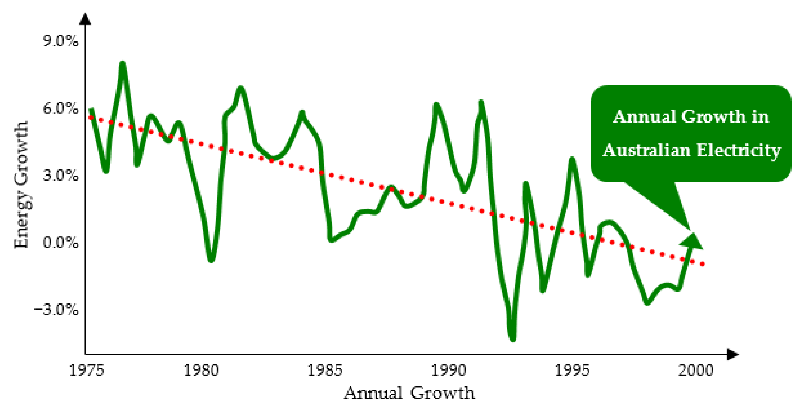
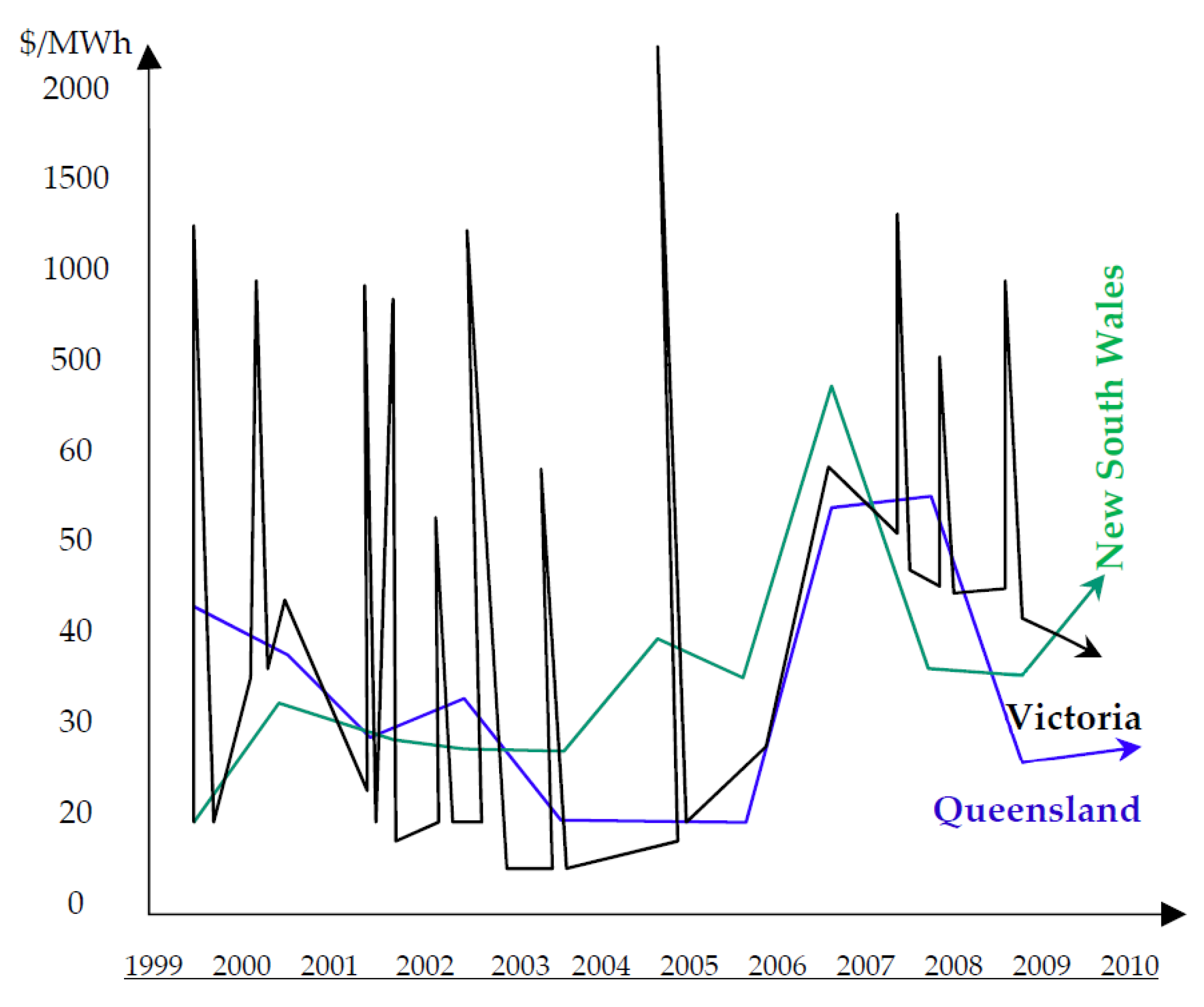
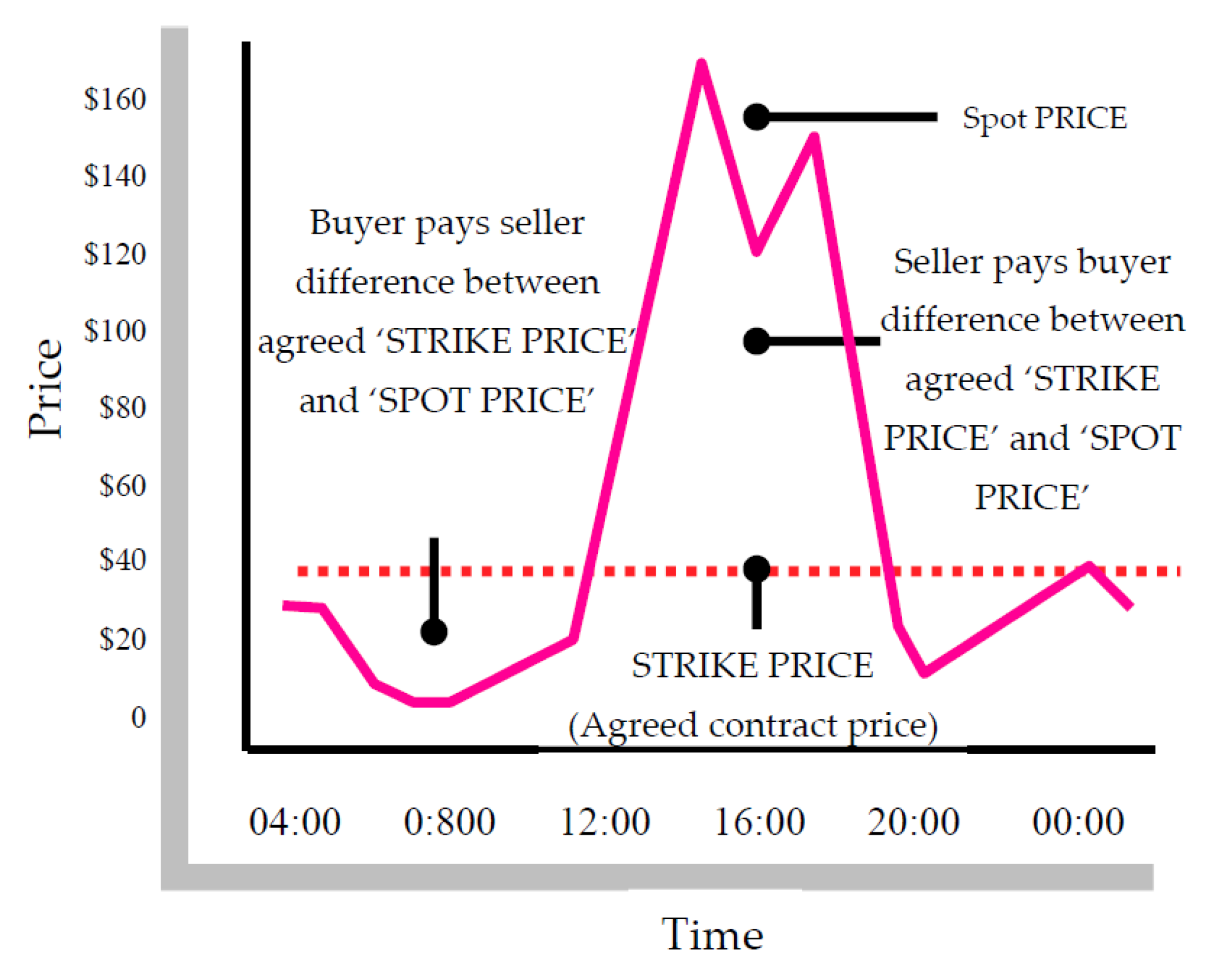
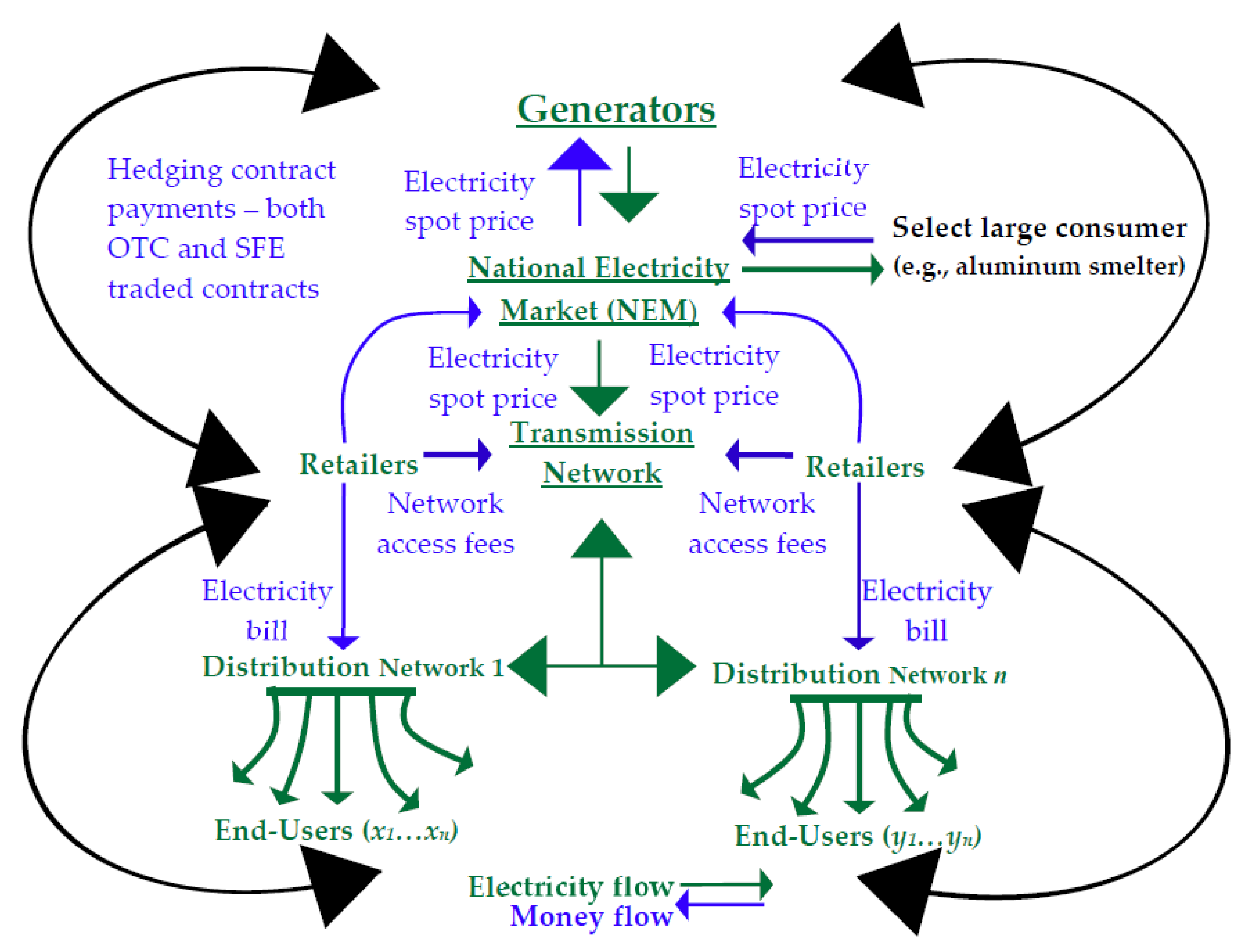
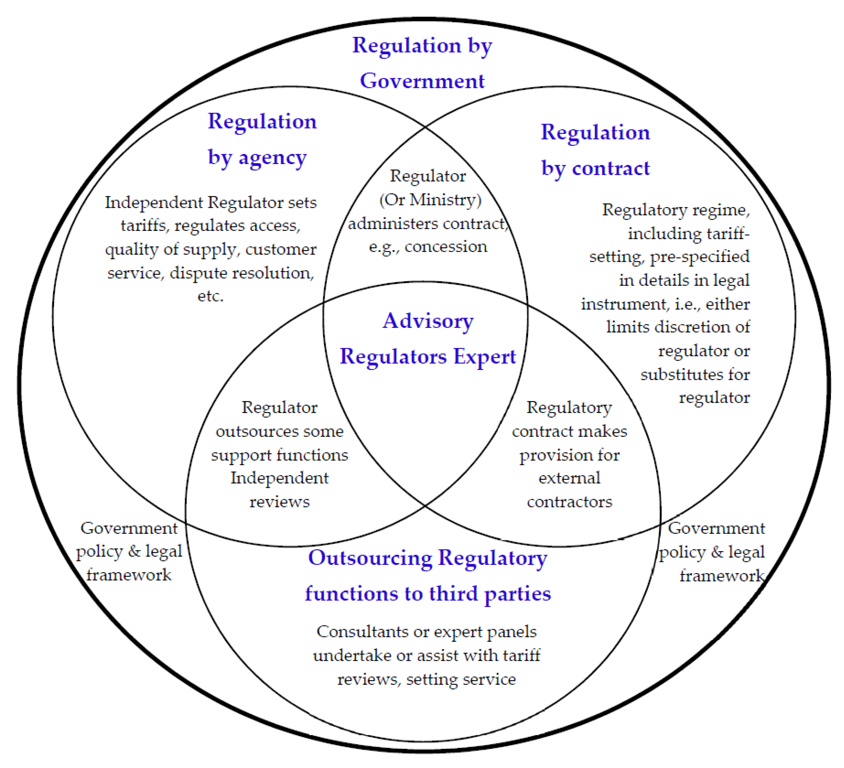
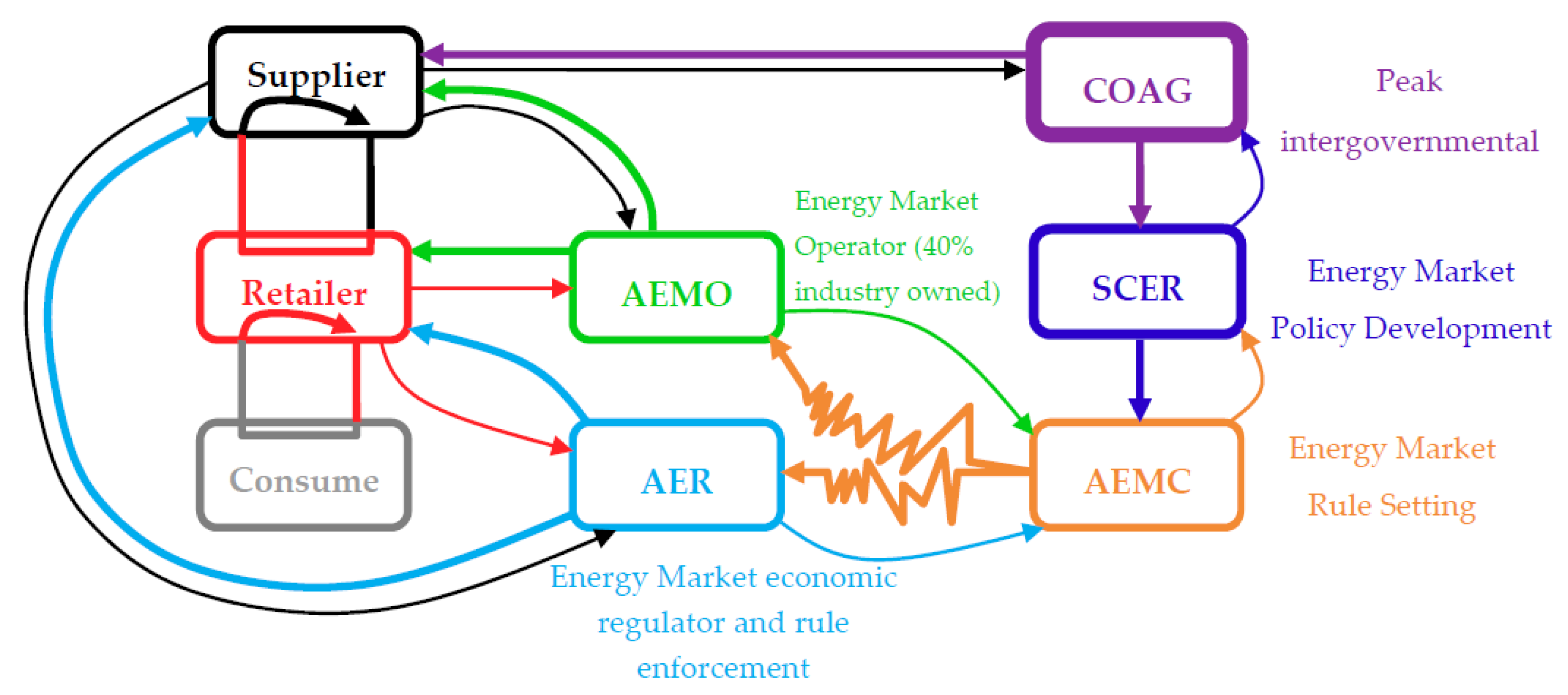
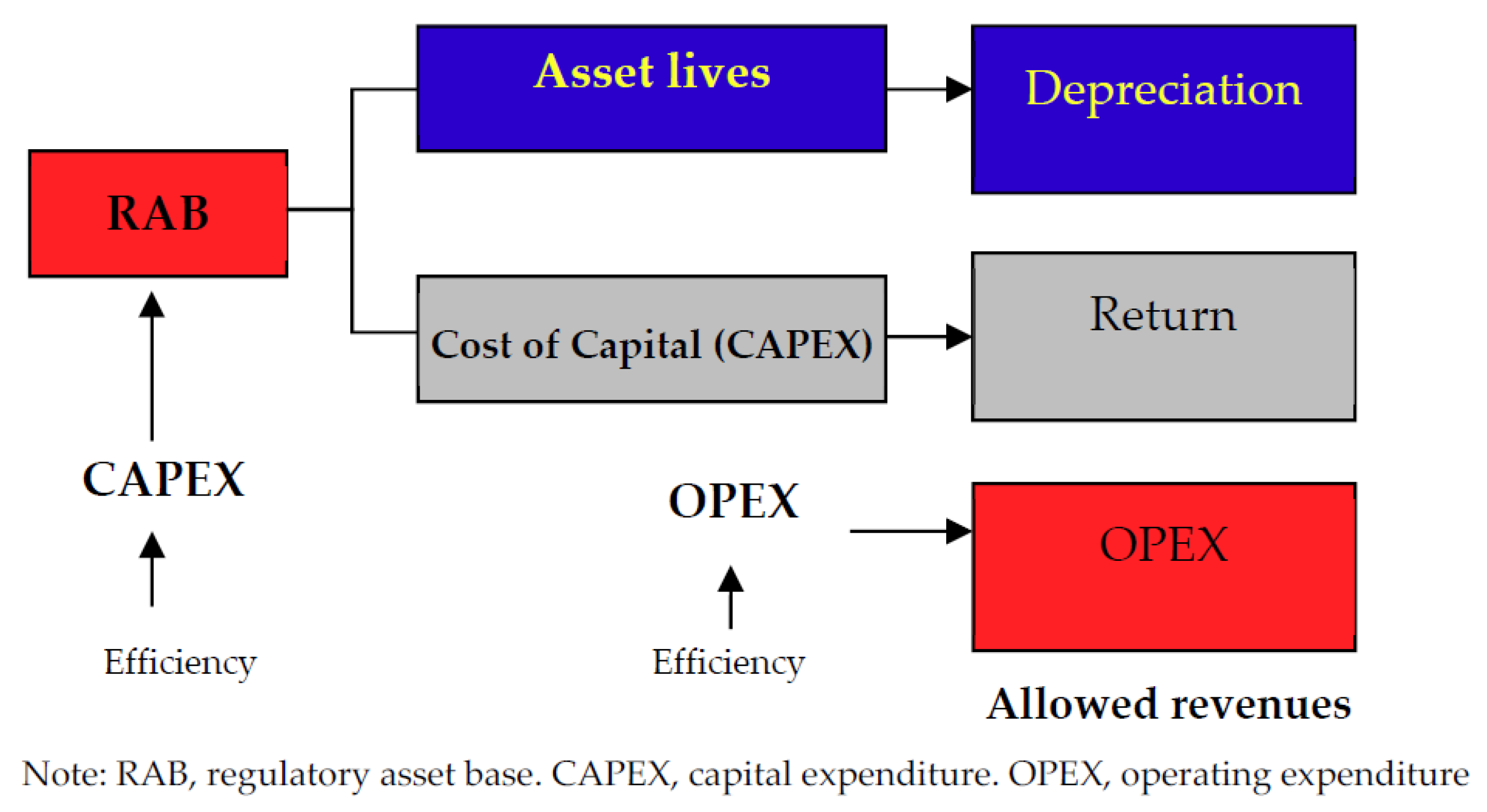
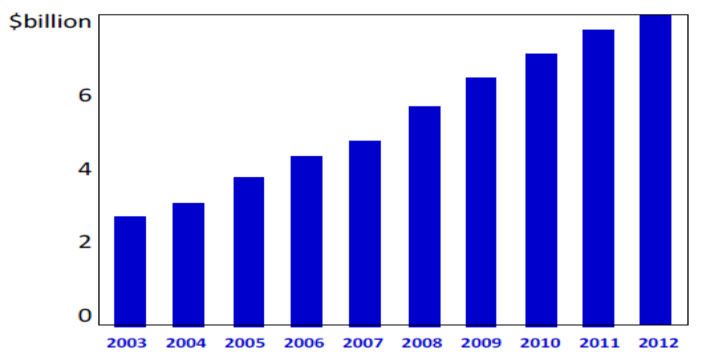
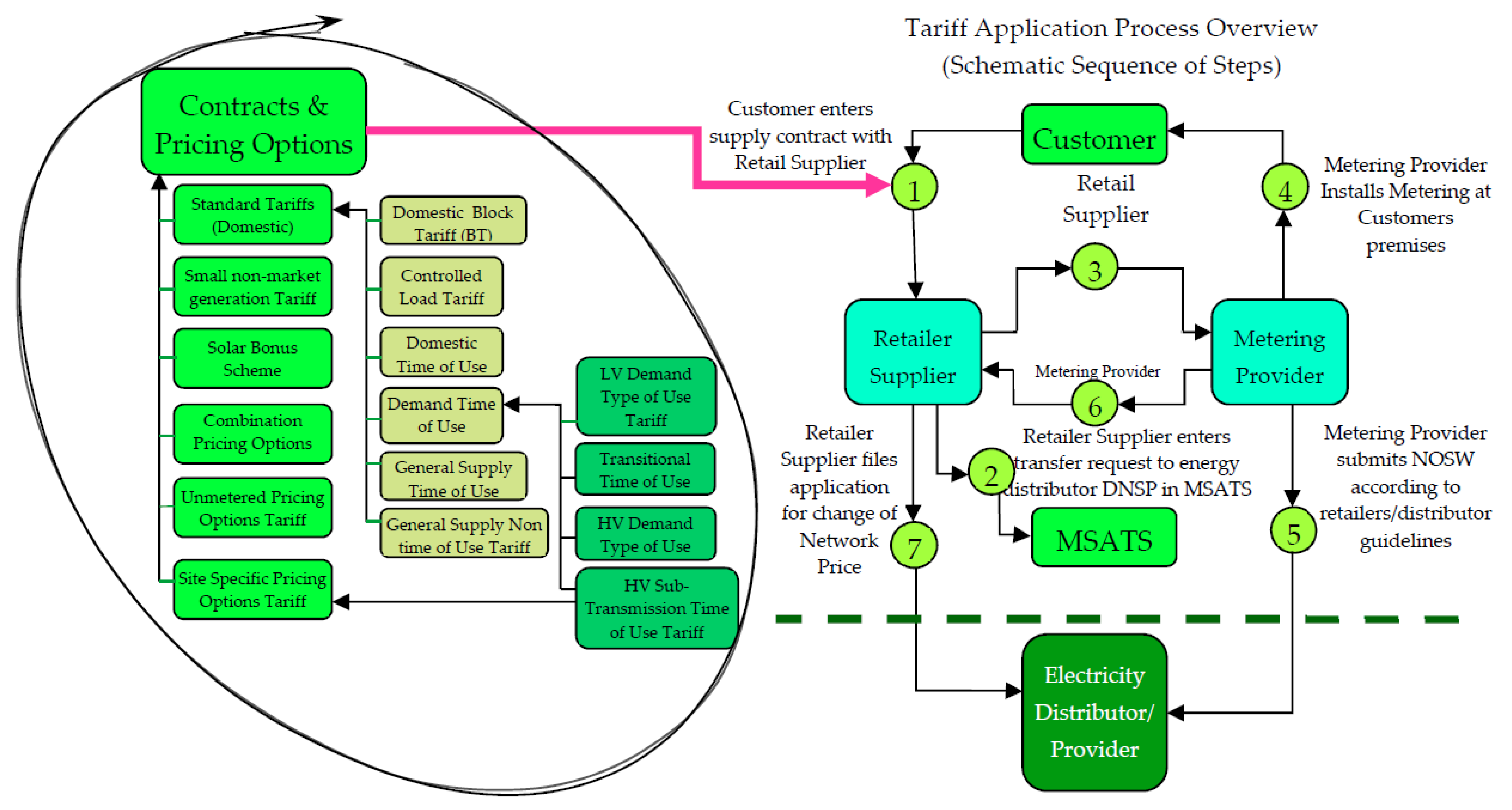
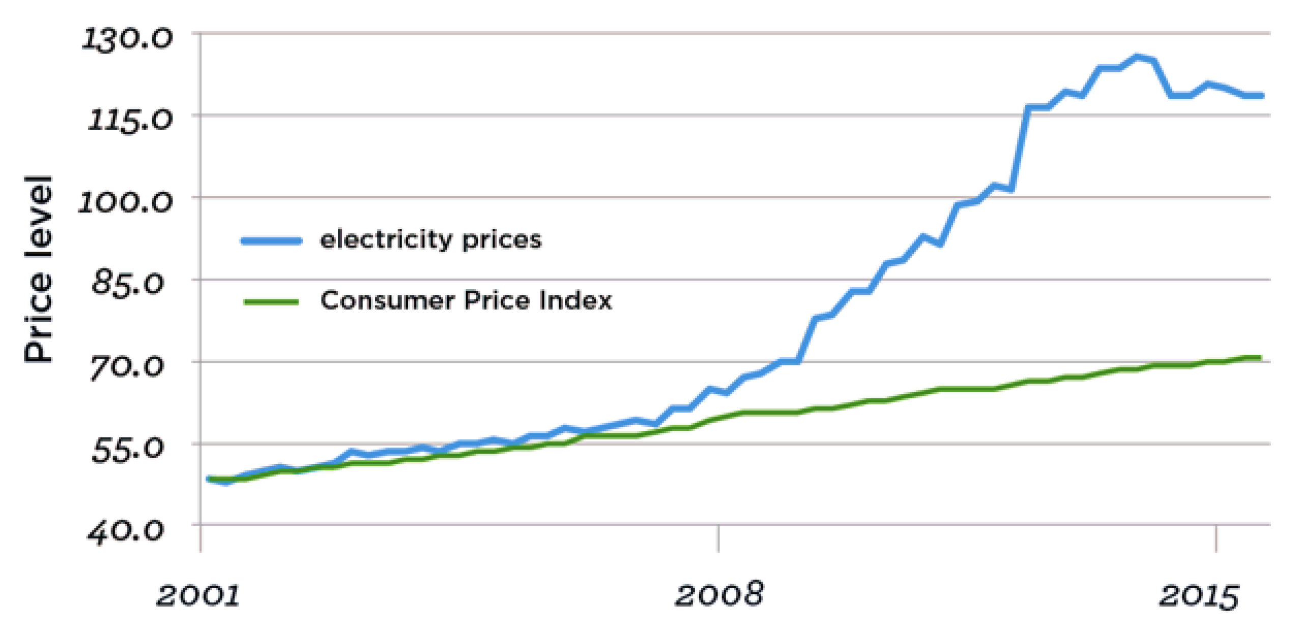
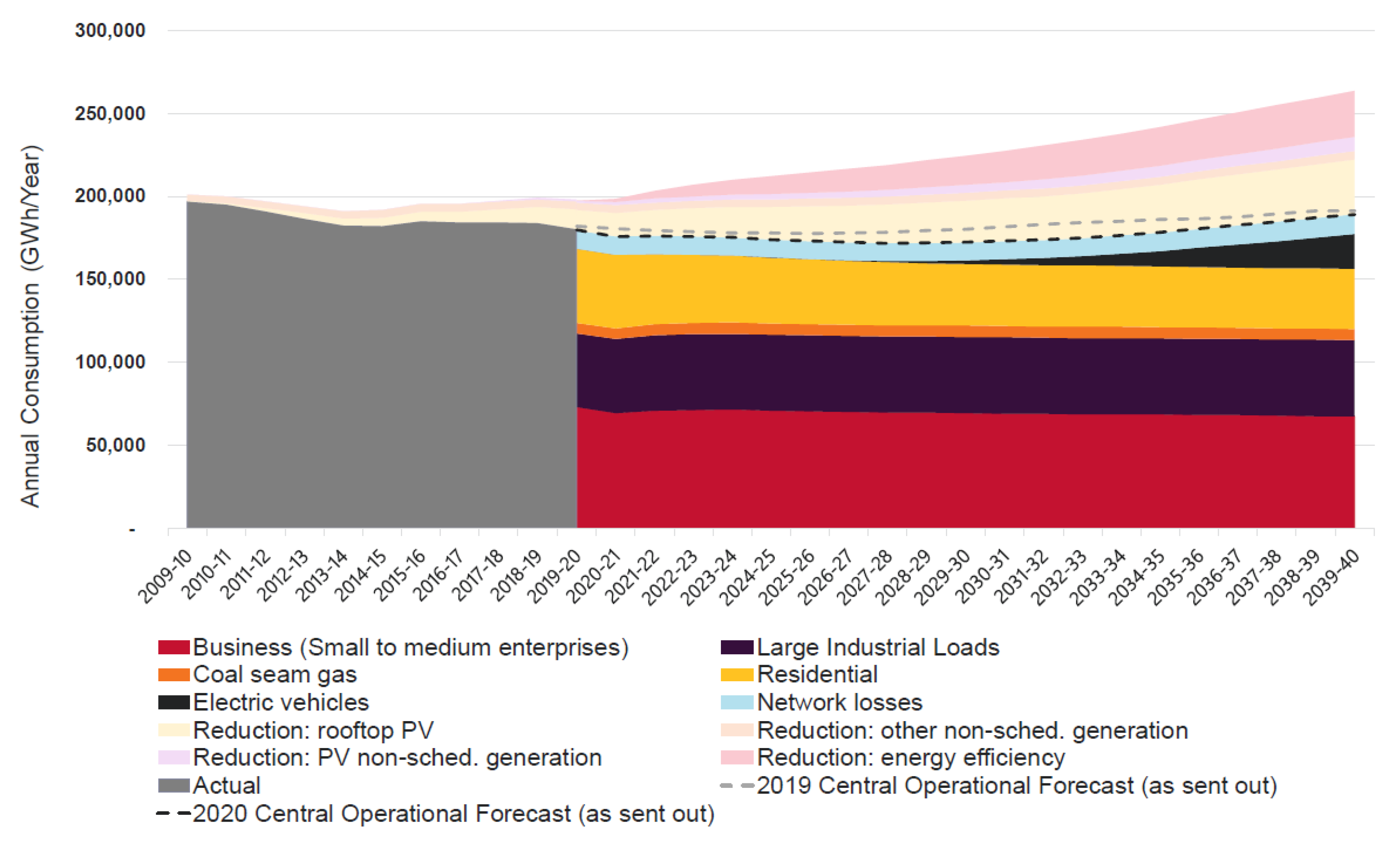
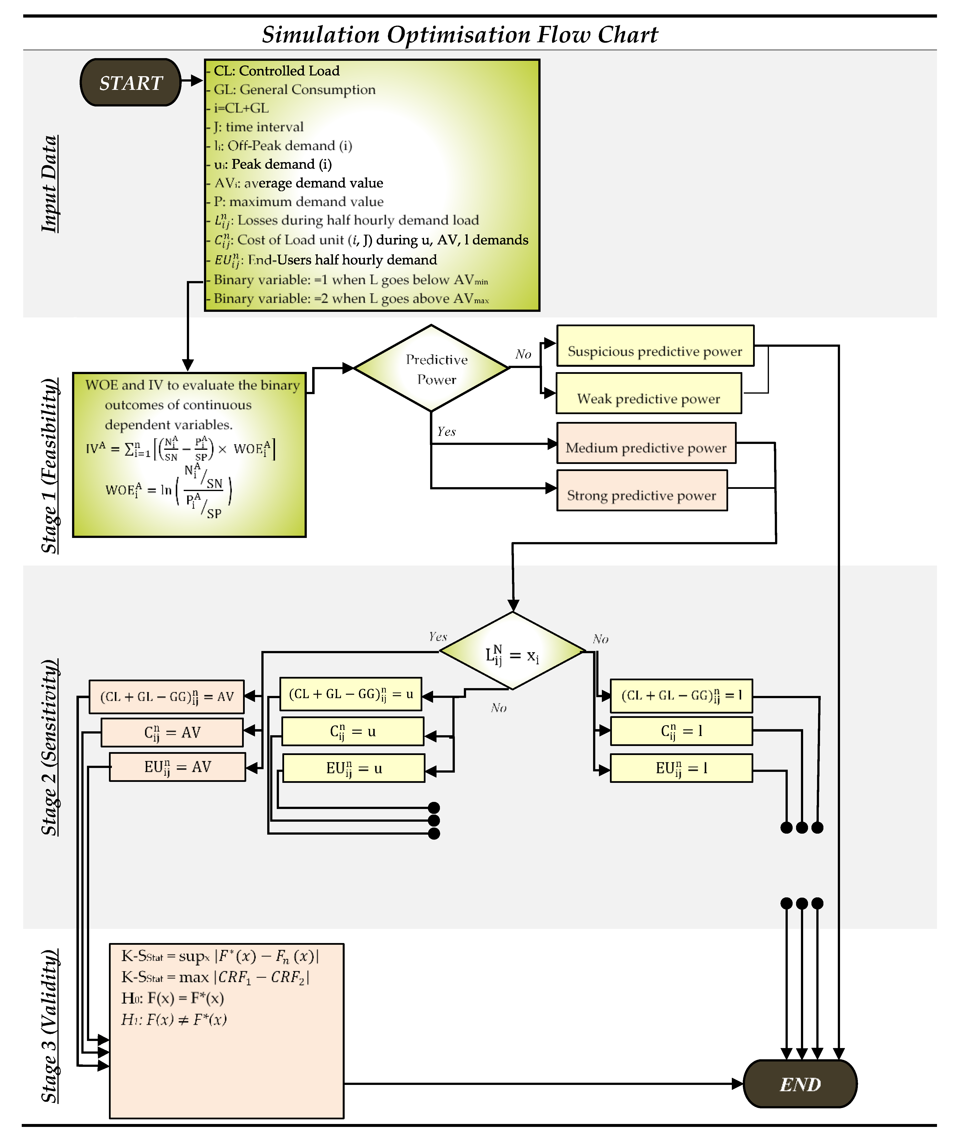
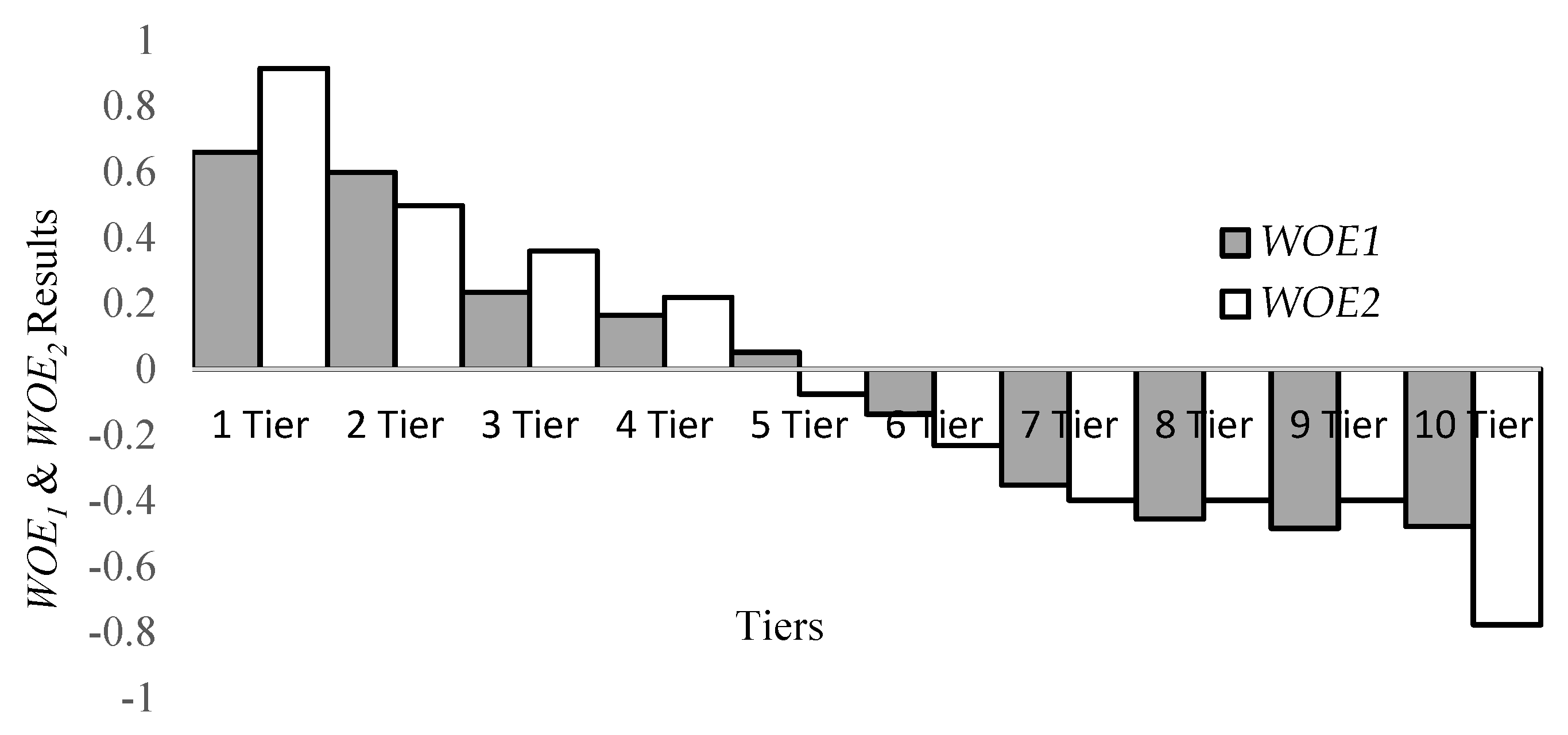
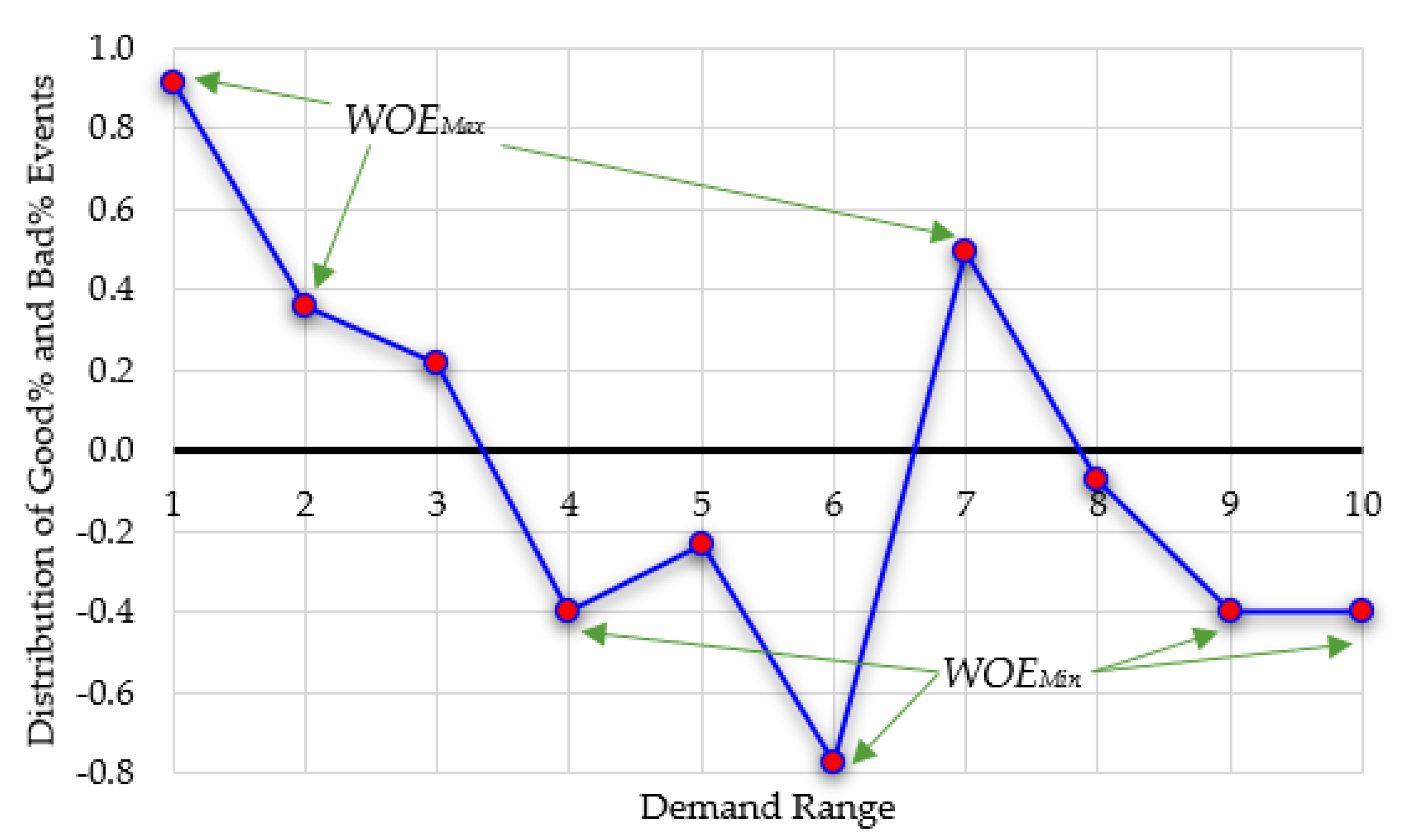
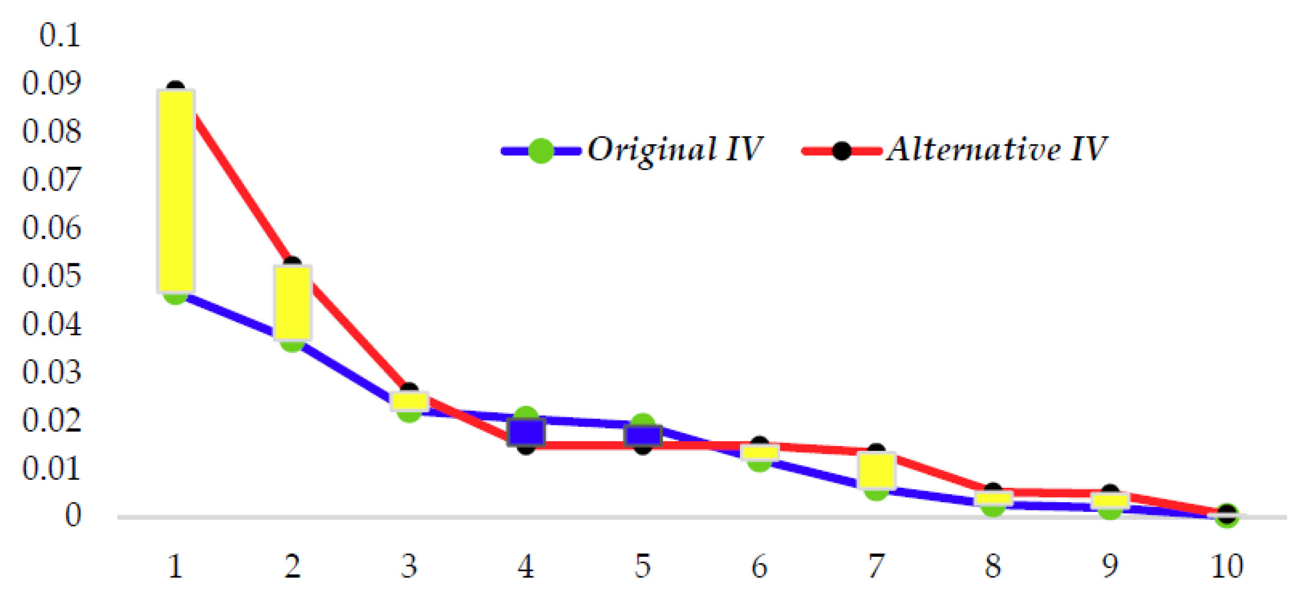
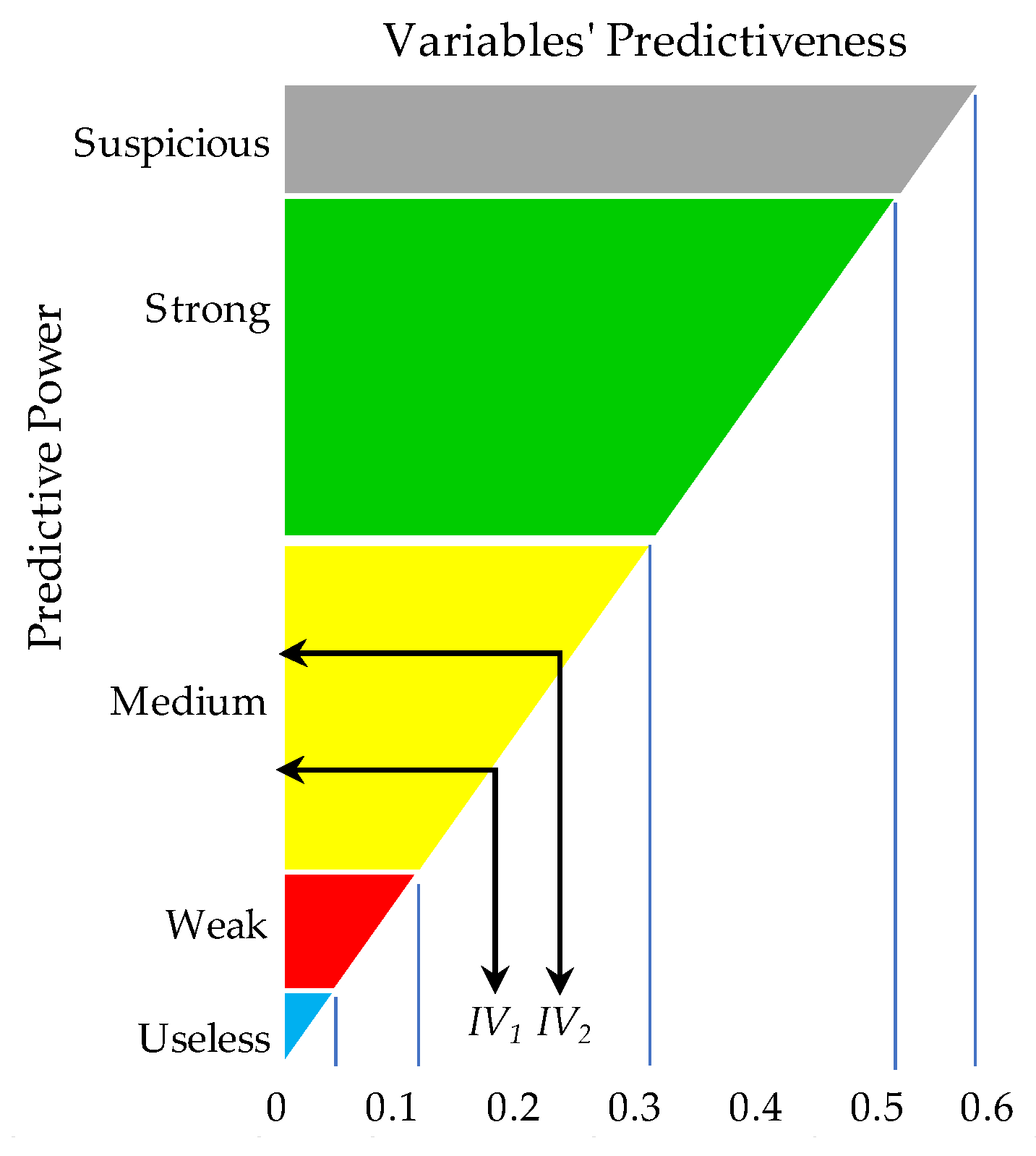
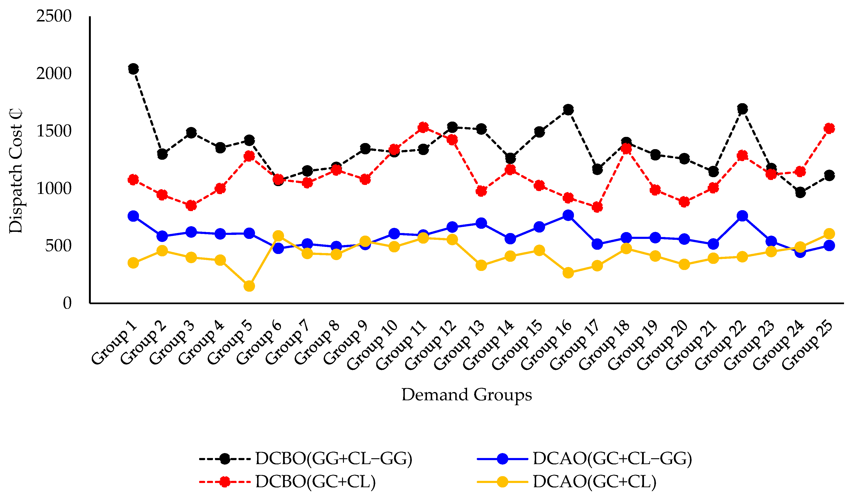
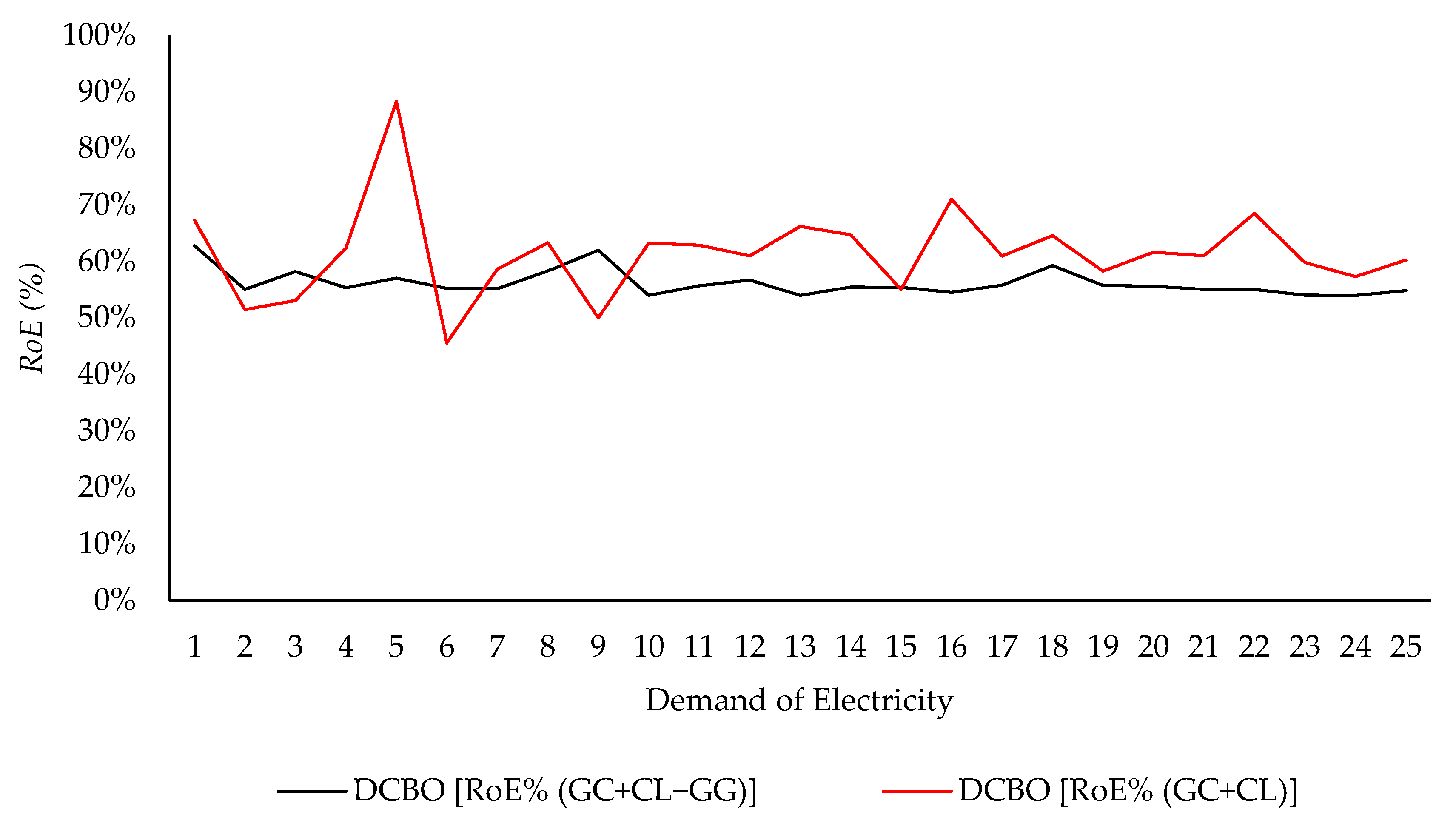
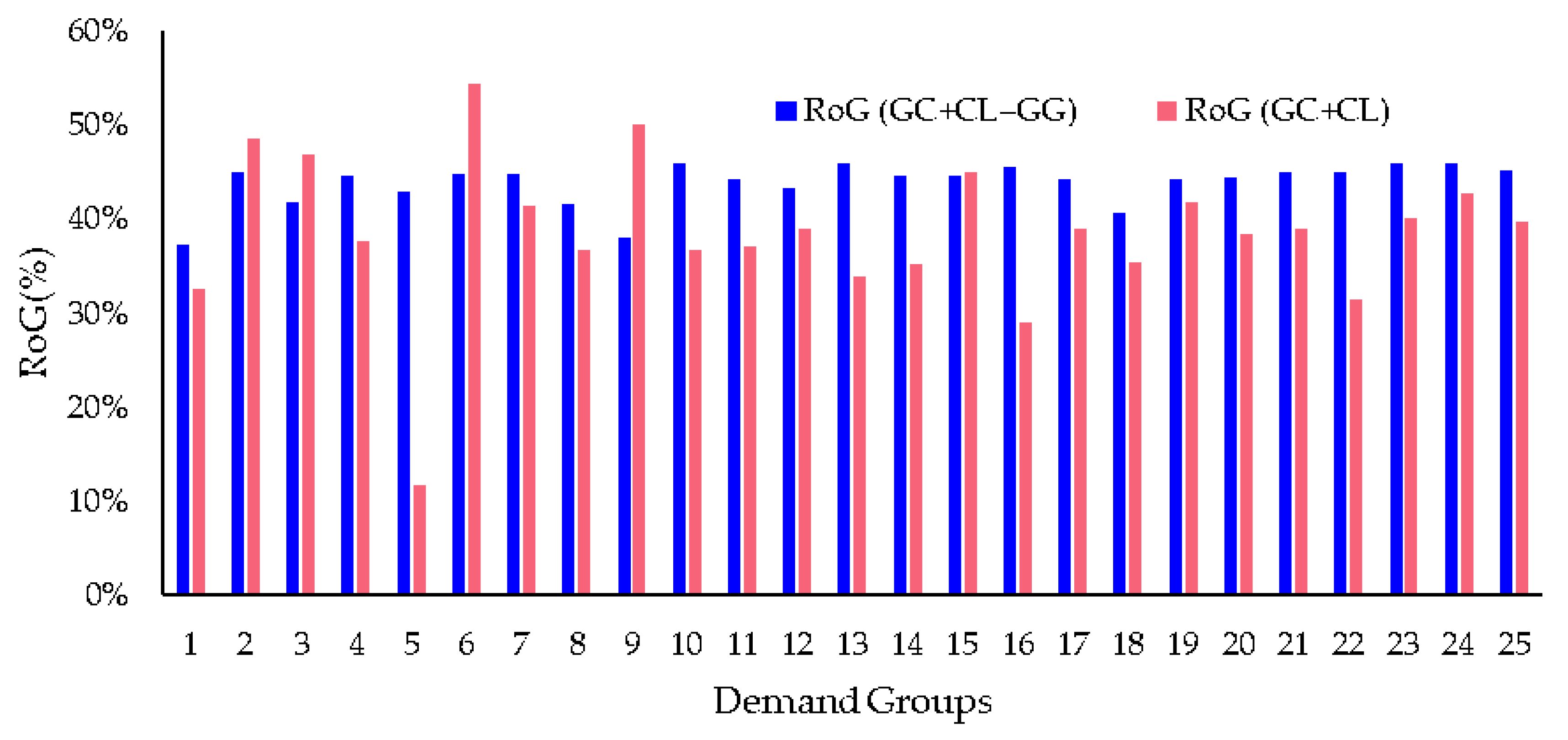
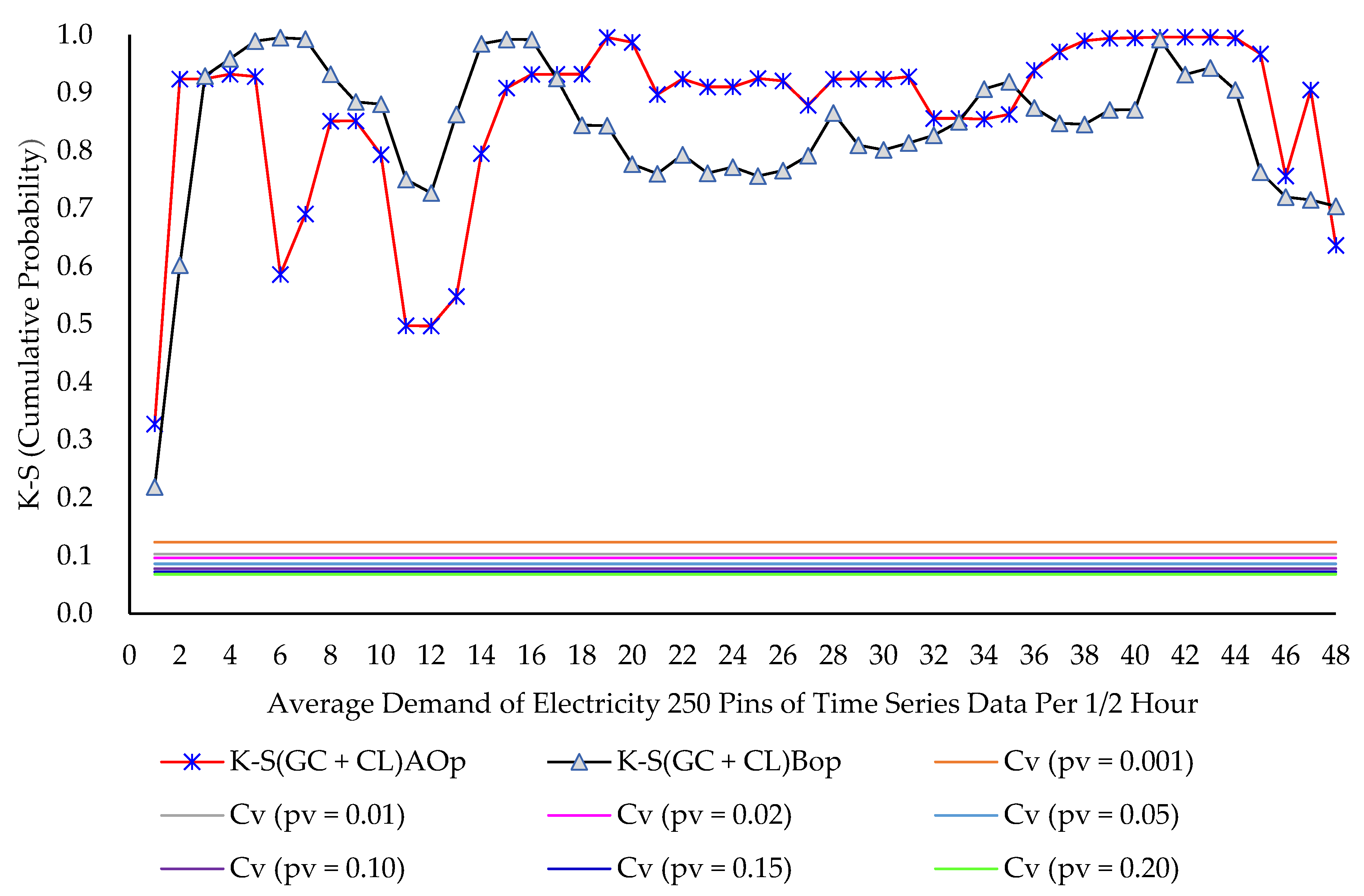
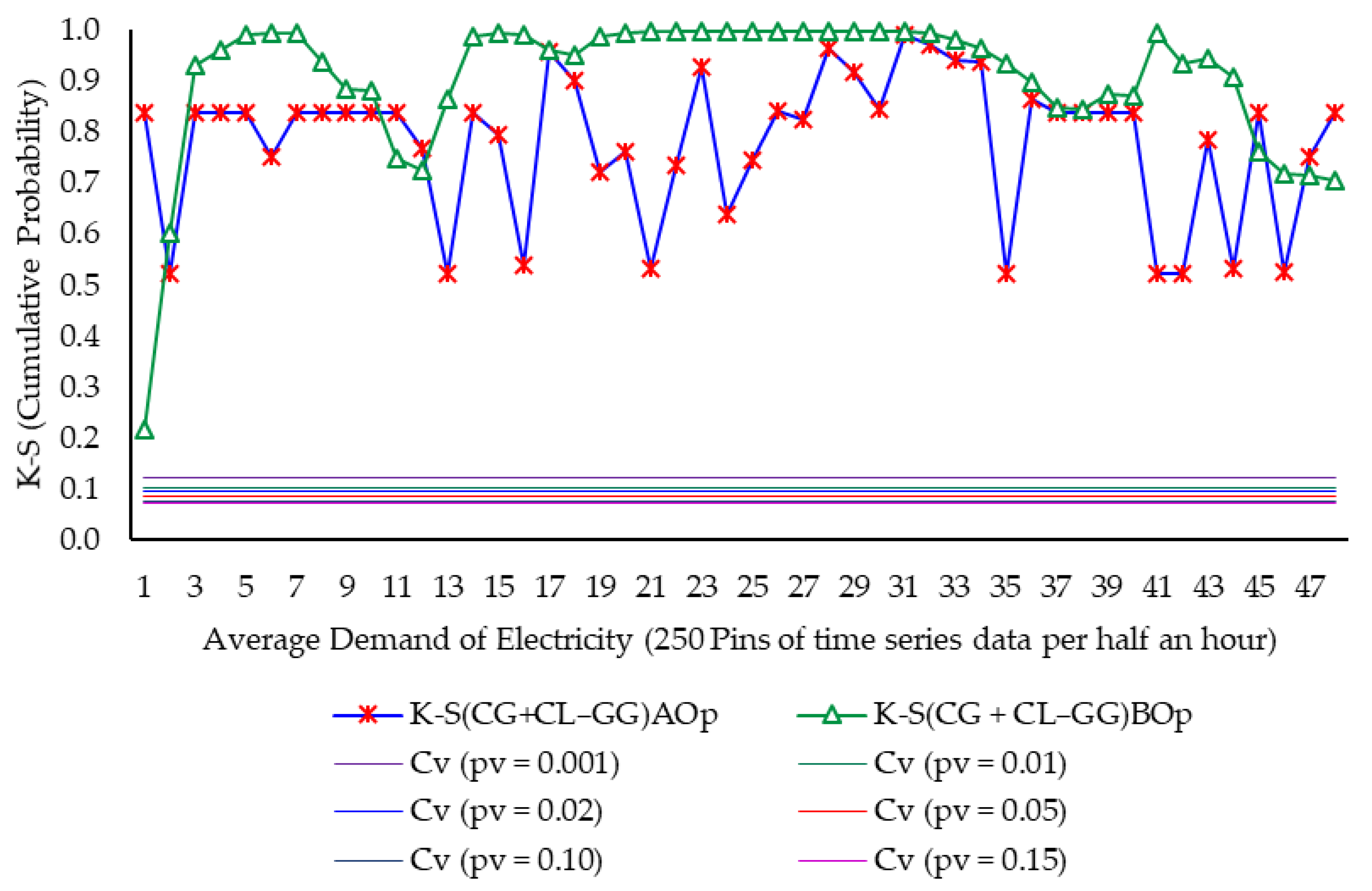
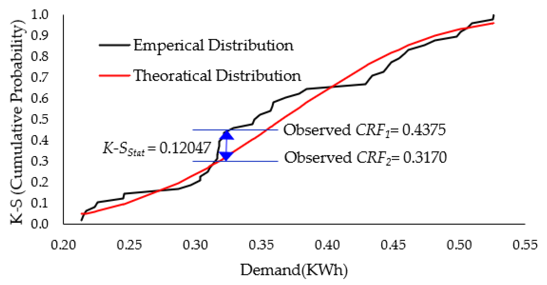
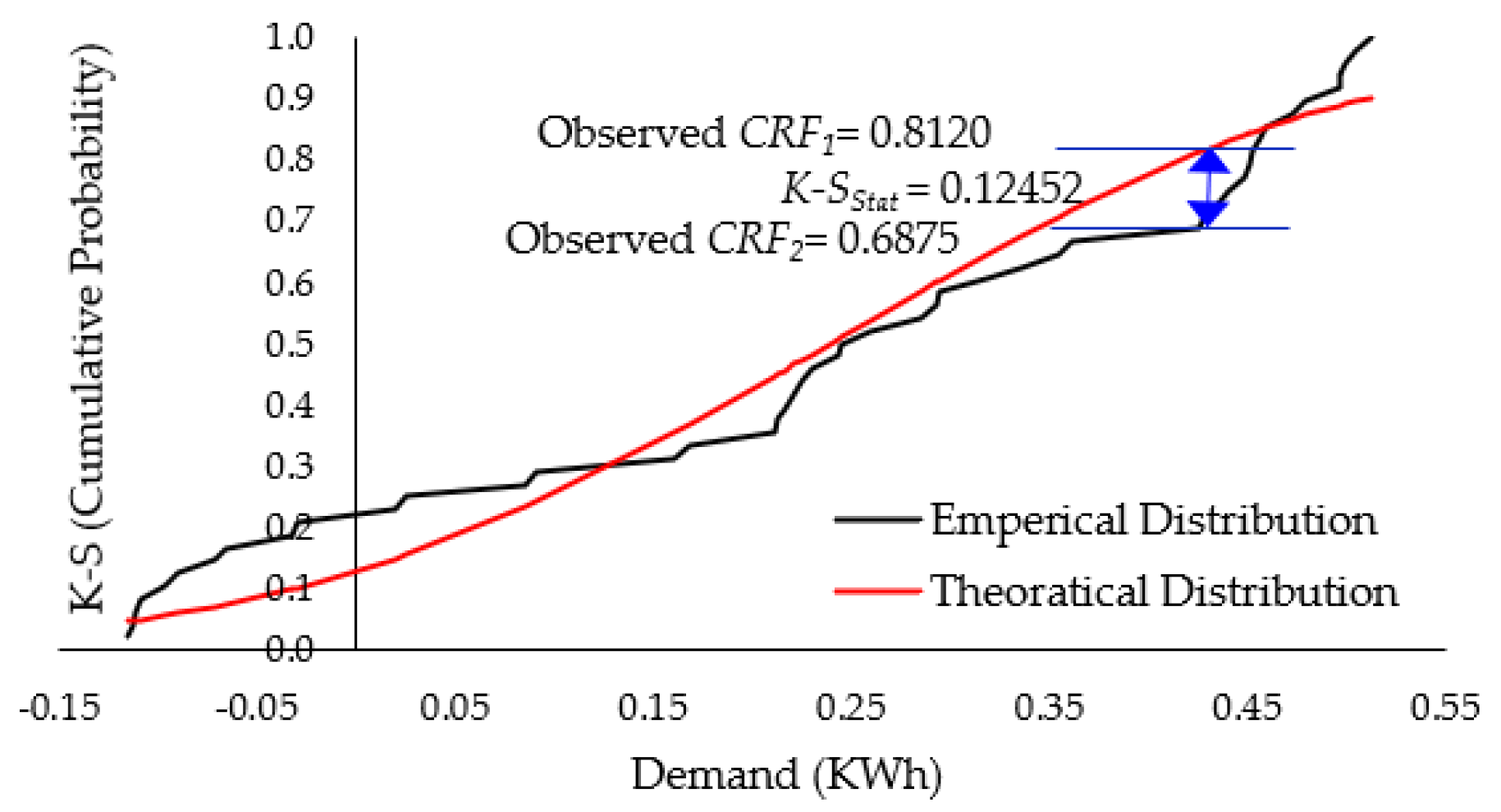
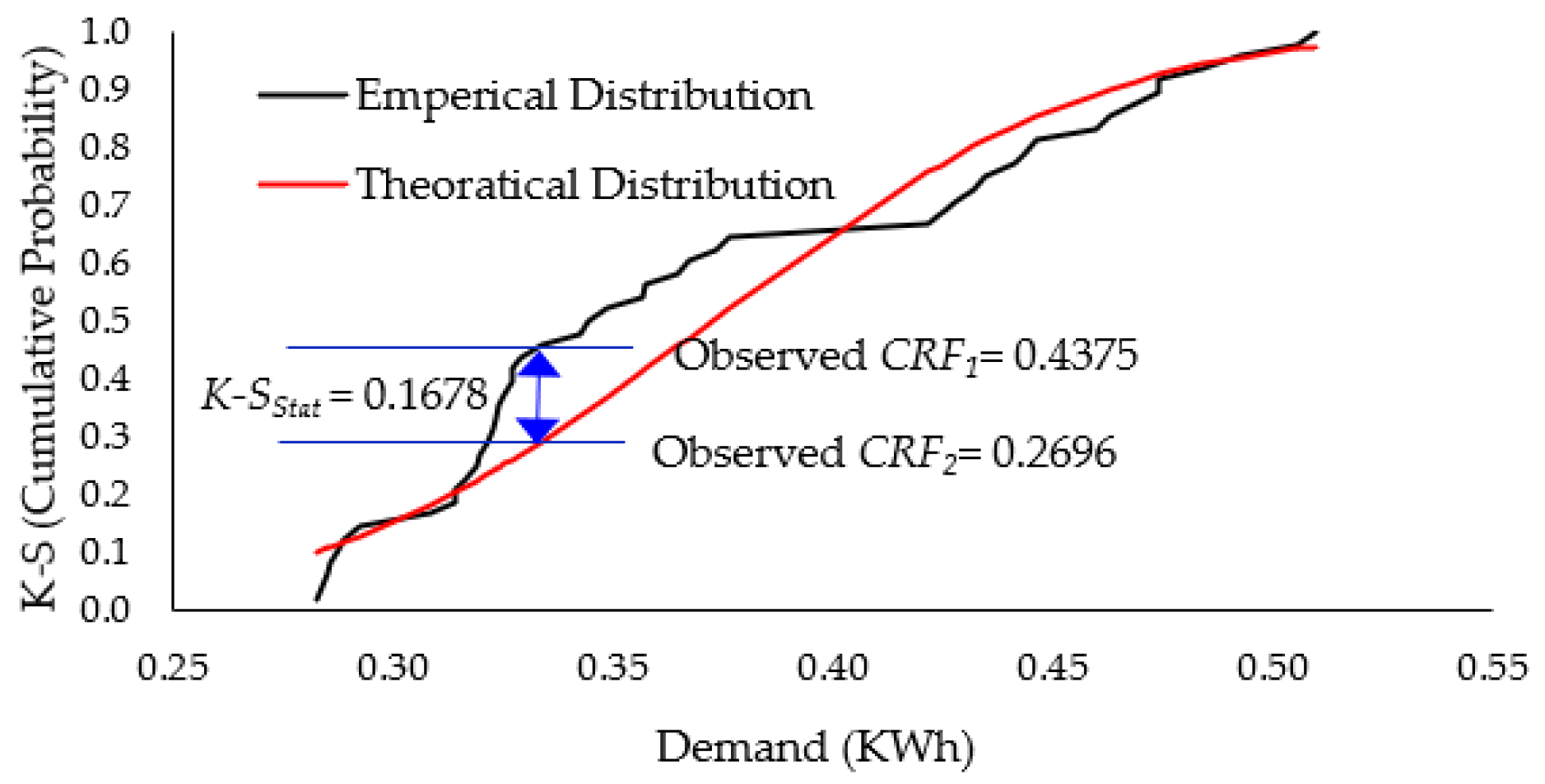
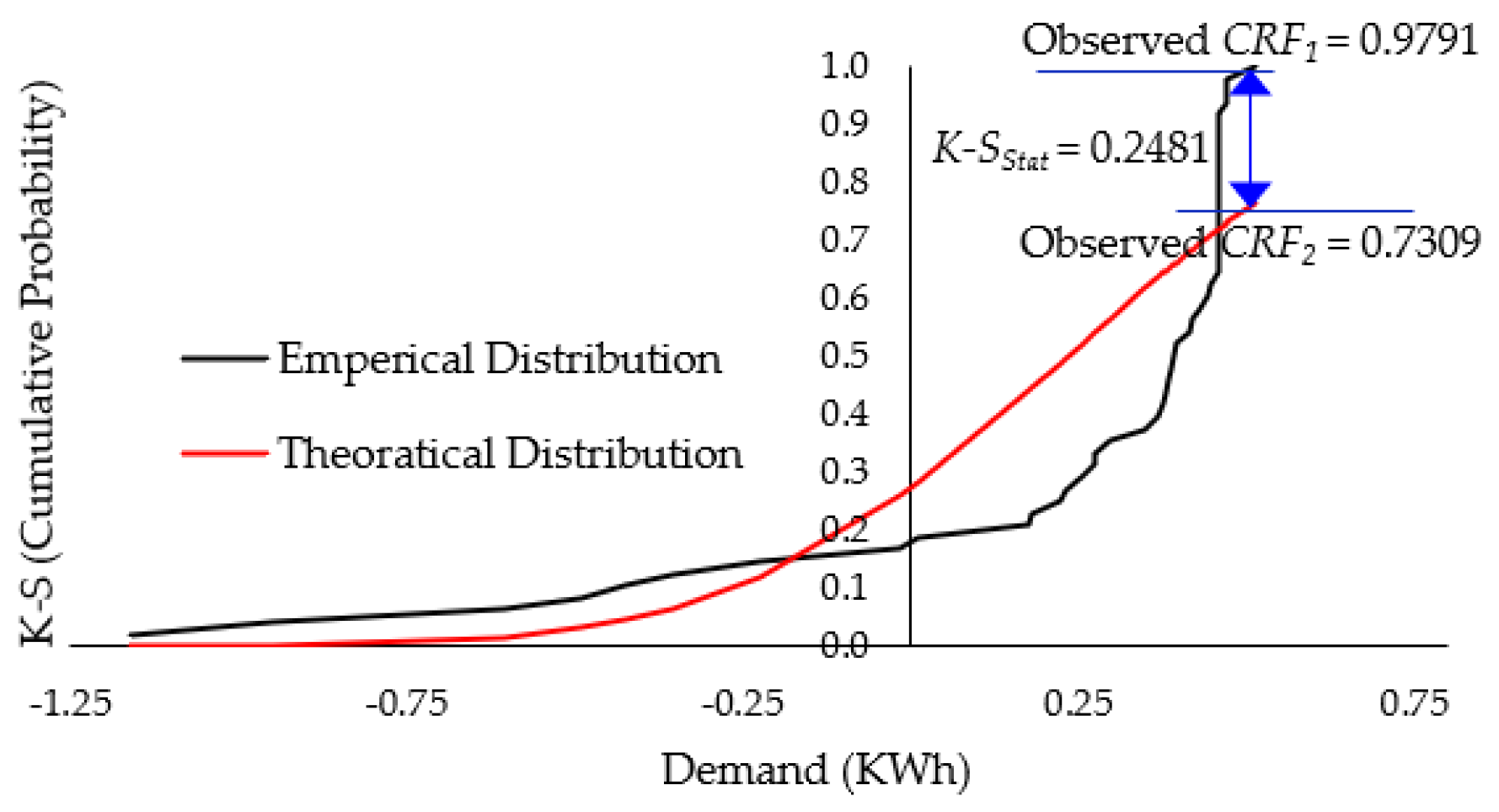
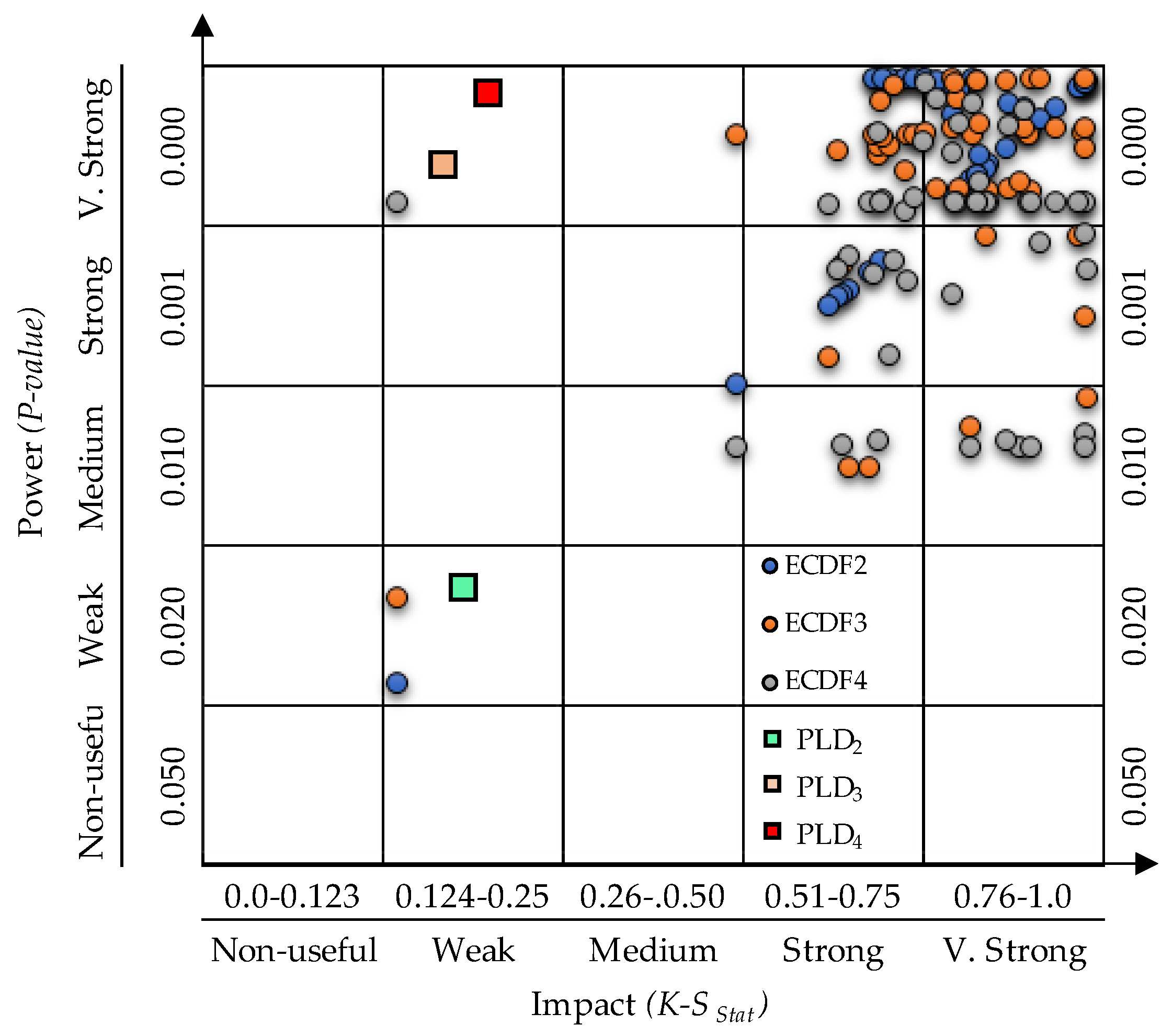
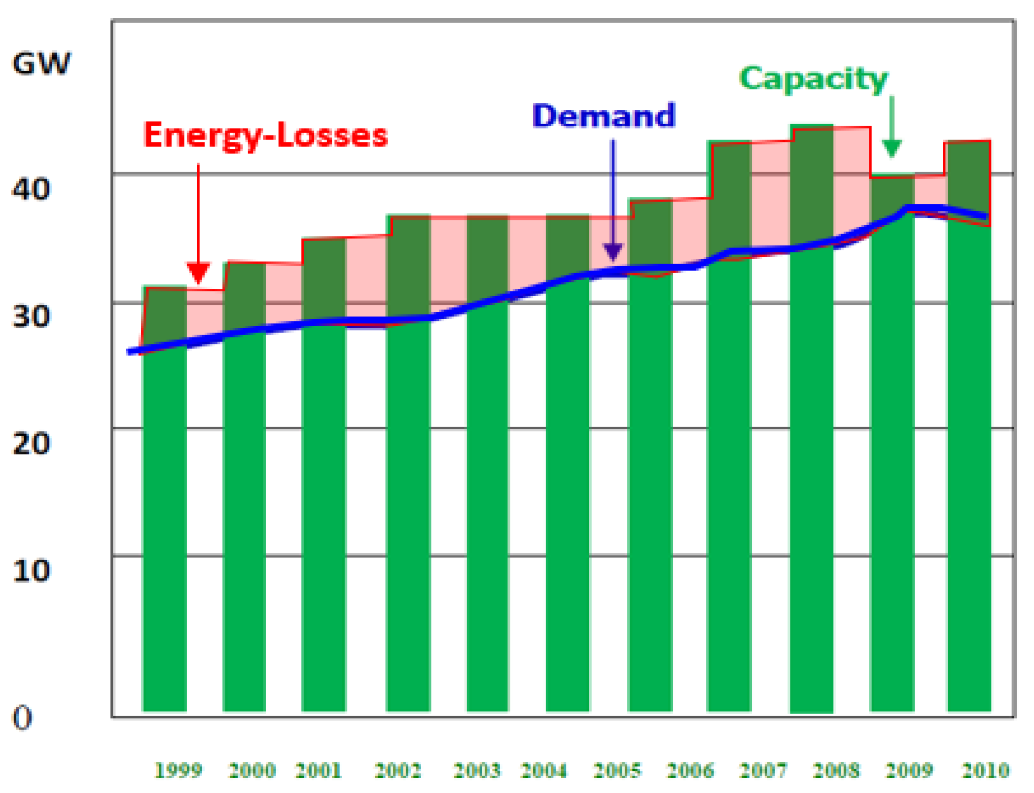
Table 1.
Recent impacts of DSM on five continents.
| Country of DSM | Evaluation Object | Indexes for End-User’s Role | Country of DSM | Evaluation Object | Indexes for End-User’s Role |
|---|---|---|---|---|---|
| Sweden and Portugal (2021) [7] | Decentralised energy storage | Demand autonomy attitudes and business models | 166 regions in Germany (2020) [17] | Independent energy autonomy from supply systems | Increasing solar by end-users adds economic benefit |
| Great Britain (2018) [8] | Decentralised, fossil fuel, and intermittent energy sources | Reliability of electricity networks | Worldwide (2021) [18] | The spectrum role of decentralised energy for inclusive economic growth | Integrate energy demand to other sources at minimum cost |
| China (2020) [9] | Decentralised framework for low emission and controlled carbon tax | Multi-stakeholder coordination with multi-energy interaction | Germany (2020) [19] | Decentralised renewable/conventional manufacturing systems | Employ residual power to control excessive charge and stabilise the grid |
| Switzerland (2019) [10] | Decentralised business options for managing generation system | Developing prosumer poses a threat to electric utilities | South Africa (2020) [20] | Decentralised RE, disempowering the grid, and local communities | RE companies’ engagement with communities is sufficient |
| Cameroon (2020) [11] | Decentralised supply/renewables to maximise output | Techno-economic benefits to end-users at low cost | California/New York in the US (2020) [21] | Solar restructuring and regulatory rules affect outcomes | The choice of Society to reinforcing solar energy and grid system integration |
| Canada and Sahara Africa (2021) [12] | Off-grid and decentralised hybrid renewable electricity systems | End-users’ access to sustainable energy | 132 islands in Philippines (2019) [22] | Centralised and decentralised electricity supply options | Interconnect renewables to submarine cable hybrid system |
| Europe North Sea Region (2021) [13] | Reinforcing grid infrastructure to manage distributed energy storage systems | A micro-energy market for smart energy trading with sustainable implementation | Great Britain (2020) [23] | Decentralised demand-side energy planning, effective real-time demand and forecasting measures | Energy plans for assets operating in domestic houses and small communities |
| US (2021) [14] | Drivers, contexts, processes, policies, and interactions affect microgrid adoption | Power outages and climate change are key pressures for the adoption of microgrids | Europe (2017) [24] | Decentralised power to avoid grid losses connected at seven voltage levels in reference to an EHV | Distribution energy loss in grid demand caused by end-users in local proximity |
| Germany (2020) [15] | Technological decentralisation and the role of the projects at the local level | Four dimensions: microgrid, location infrastructure, agility, balancing and supply | Pakistan (2021) [25] | Minimising energy cost of geo by combining intra-datacentre with a blockchain-based inter-datacentre framework | Cost of power outages, security, less demand, and inflexibility of energy dynamics |
| Bangladesh (2020) [16] | Policy implications of energy decentralisation | Adopt solar by supporting education, health, standard of living, information access and safety | Australia (2020) [26] | A multi-agent-based decentralised relaxed-constrained energy management for a microgrid | Manage demand to reduce the peak of the load by reshaping the appliance’s load |
Table 2.
Average annual growth of power generation [30]. Source: Licensed from the Commonwealth of Australia under a Creative Commons Attribution 3.0 Australia Licence.
Table 2.
Average annual growth of power generation [30]. Source: Licensed from the Commonwealth of Australia under a Creative Commons Attribution 3.0 Australia Licence.
| 2014–2015 | Average Annual Growth | |||
|---|---|---|---|---|
| GWh | Share (per Cent) | 2014–2015 (per Cent) | 10 Years (per Cent) | |
| Fossil fuels | 217,871 | 86.3 | 3.1 | 0.4 |
| Black coal | 107,639 | 42.7 | 1.8 | −2.1 |
| Brown coal | 50,970 | 20.2 | 10.6 | −0.8 |
| Gas | 52,463 | 20.8 | −3.6 | 9.7 |
| Oil | 6799 | 2.7 | 35.6 | 9.3 |
| Renewables | 34,488 | 13.7 | −6.9 | 5.3 |
| Hydro | 13,445 | 5.3 | −27.0 | −1.9 |
| Wind | 11,467 | 4.5 | 11.8 | 23.5 |
| Bioenergy | 3608 | 1.4 | 11.4 | −1.0 |
| Solar PV | 5968 | 2.4 | 22.9 | 59.3 |
| Geothermal | 1 | 0.0 | 27.3 | 2.7 |
| Total | 252,359 | 100.0 | 1.6 | 0.9 |
| Influence on Wholesale Electricity Costs | Influence on Retail Electricity Prices | Effect on Wholesale Spot Price Volatility | |
|---|---|---|---|
| Introduce more renewable generation | Decrease | Increase | Increase |
| Thermal generation retirements | Increase | Increase | Increase |
Table 4.
Goodness-of-fit tests.
| No. | Normality Test | Sensitivity and Specificity | Sample Size | Procedure |
|---|---|---|---|---|
| 1 | Pearson’s chi-square (C-S) [58] | 95% | Frequency ≥ 5 in each bin ≥30 | ‘Comparison between sample data distribution and theoretical distribution’ [58]. |
| 2 | Shapiro–Wilk (S-W) [58] | 90% | ≥55 | ‘A linear model to compare the expected values of the ordered statistics and ordered observations of the standard normal distribution’ [58]. |
| 3 | Anderson–Darling (A-D) [58] | 95% | ≥120 | ‘How close the points are to the straight line estimated in a probability’ [58]. |
| 4 | Cramér–von Mises (C-M) [36] | 95% | ≥140 | ‘Minimum distance estimation between theoretical and sample probability distribution’ [58]. |
| 5 | Jarque–Bera (J-P) [58] | 95% | ≥50 | ‘Difference estimation between asymmetry and kurtosis of observed data and theoretical distribution’ [58]. |
| 6 | Lilliefors (L-F) [58] | <(K-S) | >140 | ‘Calculation of an approximation of the sampling distribution by usinga modified KS that uses a Monte Carlo technique’ [58]. |
| 7 | D’Agostino–Pearson (A-P) [58] | 95% | ≥80 | ‘Measures combination of asymmetry and kurtosis’ [58]. |
| 8 | Jackknife (J-K) [61] | 95% | <30 | ‘Recompute the estimate from subsamples of the available sample to estimate the bias and a standard error’ [61]. |
| 9 | Kolmogorov–Smirnov (K-S) [57] | 90% | >140 | ‘Proximity analysis applied between the hypothesised theoretical distribution and the empirical sample distribution’ [57]. |
Table 5.
WOE, IV, and %Bad Rate.
| Range | Pins | Records | Good | Bad | No Events | Events | WOE1 | WOE2 | IV1 | IV2 | % Bad Rate |
|---|---|---|---|---|---|---|---|---|---|---|---|
| 0–29 | 1 | 507.9450 | 259.1380 | 248.8069 |  |  |  |  | 0.0467 | 0.0260 |  |
| 30–58 | 2 | 487.5548 | 241.2927 | 246.2621 | 0.0368 | 0.0134 | |||||
| 59–87 | 3 | 530.3947 | 214.7703 | 315.6244 | 0.0059 | 0.0049 | |||||
| 88–116 | 4 | 482.3963 | 187.1223 | 295.2740 | 0.0026 | 0.0888 | |||||
| 117–145 | 5 | 470.2308 | 170.1727 | 300.0580 | 0.0003 | 0.0006 | |||||
| 146–174 | 6 | 537.6337 | 171.7984 | 365.8354 | 0.0020 | 0.0052 | |||||
| 175–203 | 7 | 514.0614 | 141.1246 | 372.9367 | 0.0119 | 0.0149 | |||||
| 204–232 | 8 | 540.2302 | 137.5412 | 402.6890 | 0.0204 | 0.0149 | |||||
| 233–261 | 9 | 533.8289 | 133.5758 | 400.2532 | 0.0222 | 0.0149 | |||||
| >261 | 10 | 445.9397 | 111.0922 | 334.8475 | 0.0190 | 0.0522 | |||||
| Total | 5050.2154 | 1767.6282 | 3282.5872 | 105 | 185 | 0.1677 | 0.2357 |
Table 6.
Traditional demand before optimisation (GC+CL)Bop.
| p-value | 0.001 | 0.01 | 0.02 | 0.05 | 0.1 | 0.15 | 0.2 |
| K-Sstat | 0.12047 | 0.12047 | 0.12047 | 0.12047 | 0.12047 | 0.12047 | 0.12047 |
| C-value | 0.12329 | 0.10293 | 0.09597 | 0.08589 | 0.07740 | 0.07197 | 0.06784 |
| Cv > k-S | Cv < k-SStat | Cv < k-S | Cv < k-S | Cv < k-S | Cv < k-S | Cv < k-S |
Table 7.
(GC+CL−GG)Bop.
| p-value | 0.001 | 0.01 | 0.02 | 0.05 | 0.1 | 0.15 | 0.2 |
| K-Sstat | 0.12452 | 0.12452 | 0.12452 | 0.12452 | 0.12452 | 0.12452 | 0.12452 |
| C-value | 0.12329 | 0.10293 | 0.09597 | 0.08589 | 0.07740 | 0.07197 | 0.06784 |
| Cv < k-S | Cv < k-S | Cv < k-S | Cv < k-S | Cv < k-S | Cv < k-S | Cv < k-S |
Table 8.
(GC+CL)AOp.
| p-value | 0.001 | 0.01 | 0.02 | 0.05 | 0.1 | 0.15 | 0.2 |
| K-Sstat | 0.16786 | 0.16786 | 0.16786 | 0.16786 | 0.16786 | 0.16786 | 0.16786 |
| C-value | 0.12329 | 0.10293 | 0.09597 | 0.08589 | 0.07740 | 0.07197 | 0.06784 |
| Cv < k-S | Cv < k-S | Cv < k-S | Cv < k-S | Cv < k-S | Cv < k-S | Cv < k-S |
Table 9.
(GC+CL−GG)AOp.
| p-value | 0.001 | 0.01 | 0.02 | 0.05 | 0.1 | 0.15 | 0.2 |
| K-Sstat | 0.24817 | 0.24817 | 0.24817 | 0.24817 | 0.24817 | 0.24817 | 0.24817 |
| C-value | 0.12329 | 0.10293 | 0.09597 | 0.08589 | 0.07740 | 0.07197 | 0.06784 |
| Cv < k-S | Cv < k-S | Cv < k-S | Cv < k-S | Cv < k-S | Cv < k-S | Cv < k-S |
Publisher’s Note: MDPI stays neutral with regard to jurisdictional claims in published maps and institutional affiliations. |
© 2021 by the authors. Licensee MDPI, Basel, Switzerland. This article is an open access article distributed under the terms and conditions of the Creative Commons Attribution (CC BY) license (https://creativecommons.org/licenses/by/4.0/).
Share and Cite
MDPI and ACS Style
Zaghwan, A.; Gunawan, I. Energy Loss Impact in Electrical Smart Grid Systems in Australia. Sustainability 2021, 13, 7221. https://doi.org/10.3390/su13137221
AMA Style
Zaghwan A, Gunawan I. Energy Loss Impact in Electrical Smart Grid Systems in Australia. Sustainability. 2021; 13(13):7221. https://doi.org/10.3390/su13137221
Chicago/Turabian StyleZaghwan, Ashraf, and Indra Gunawan. 2021. "Energy Loss Impact in Electrical Smart Grid Systems in Australia" Sustainability 13, no. 13: 7221. https://doi.org/10.3390/su13137221
Note that from the first issue of 2016, this journal uses article numbers instead of page numbers. See further details here.