Article

Spatiotemporal Dynamics of Snowline Altitude and Their Responses to Climate Change in the Tienshan Mountains, Central Asia, during 2001–2019

1
Hunan Provincial Key Laboratory of Geo-Information Engineering in Surveying, Mapping and Remote Sensing, Hunan University of Science and Technology, Xiangtan 411201, China
2
State Key Laboratory of Cryospheric Science, Northwest Institute of Eco-Environment and Resources, Chinese Academy of Sciences, Lanzhou 730000, China
3
National-Local Joint Engineering Laboratory of Geo-Spatial Information Technology, Hunan University of Science and Technology, Xiangtan 411201, China
4
School of Resource Environment and Safety Engineering, Hunan University of Science and Technology, Xiangtan 411201, China
*
Author to whom correspondence should be addressed.
Sustainability 2021, 13(7), 3992; https://doi.org/10.3390/su13073992
Submission received: 14 January 2021 / Revised: 28 March 2021 / Accepted: 30 March 2021 / Published: 2 April 2021
(This article belongs to the Section Air, Climate Change and Sustainability)

Abstract

:
Snow cover is an important water resource in arid and semi-arid regions of Central Asia, and is related to agricultural and livestock production, ecosystems, and socio-economic development. The snowline altitude (SLA) is a significant indicator for monitoring the changes in snow cover in mountainous regions under the changing climate. Here, we investigate the spatiotemporal variation of SLA in the Tienshan Mountains (TS) during 2001–2019 using Moderate Resolution Imaging Spectroradiometer (MODIS) snow cover products on a grid-by-grid basis. The potential influence of topographic factors (slope gradient and aspect) on SLA and the correlation between SLA, temperature, precipitation, and solar radiation are also investigated. The results are as follows: (1) The annual cycle of SLA shows strong seasonal fluctuations (from about 2000 m in late December to 4100 m in early August). The SLA over the TS exhibits a large spatiotemporal heterogeneity. (2) SLA increases with a steeper slope gradient. The SLA of the northerly aspect is generally less than the southerly. (3) The SLA over the TS generally shows an increasing trend in the recent years (2001–2019). The change trend of SLA varies in different months. Except for a slight decrease in June, the SLA increased in almost all months, especially at the start of the melt season (March and April) and the end of melting season (July and August). (4) The SLA increases with increased temperature/radiation in the TS, and decreases with increased precipitation. Solar radiation is the dominant climatic factor affecting the changes of SLA in the TS. Compared with precipitation, temperature is more correlated to SLA dynamics.

1. Introduction

Snow cover is an important component of the cryosphere, as well as an indispensable variable in the study of earth system science and climate change. Snow is highly dynamic and has a great influence on land surface energy budgets and atmospheric circulation patterns due to high albedo and good thermal insulation [1,2,3,4,5]. Under the background of global warming, changes in snow cover will lead to ecological and environmental problems such as a reduction of water availability, extreme weather events, and frequent disasters, profoundly affecting the ecosystem and sustainable socio-economic development of the countries and regions concerned [6,7], which has received widespread attention from these countries. The snowline is identified as the boundary separating snow-covered areas from snow-free areas [8,9,10]. Due to the patchiness of the snow cover edge, it is also defined as a narrow belt that represents a zone of ∼50% snow coverage [9,11,12]. As an important indicator of climate change, snowline can reflect the increase and reduction of snow, and it can also comprehensively reflect the basic state of the climate and environment of mountains, plateaus, and polar regions that lack meteorological stations [13].
The snowline altitude (SLA) is a valuable metric that integrates the competing effects of snow accumulation and melt, and it can be used to assess future changes in snow cover [1,14]. Regional SLA and its inter- and intra-annual variability are key characteristics that indicate temporal variation in snow cover and duration of snow melt, and help in assessing the hydrologic cycle balance [15]. For the estimation of snow-covered area and its temporal evolution, SLA can be used as an input for hydrological modeling or validation of snow model simulations [16,17]. Besides, SLA estimates can be applied to remove clouds from satellite snow cover products [18,19]. The SLA at the end of the melting season can also serve as a good proxy for the equilibrium line altitude (ELA) on glaciers, where much of the remaining end of summer snow cover is located, and therefore for glacier mass balance [20,21,22,23,24,25].
Central Asia is the core area of the Silk Road economic belt. As the places most distanced from the oceans in the Eurasian continent, the Tienshan Mountains (TS) are called the water tower of Central Asia. They consist of a series of high mountains, basins, and valleys, boasting one of the most developed glacier mountains in the world [26,27]. Major rivers recharged by glacier/snow melt water originating from the TS (e.g., the Ili River, Syr Darya River, Amu Darya River, Tarim River, and Chu River) feed the lowland areas of Kazakhstan, Kyrgyzstan, Uzbekistan, and China’s north-western Xinjiang Uyghur Autonomous Region, which together form one of the largest irrigated areas in the world [26,28,29]. Spatiotemporal variations of the snow cover in the TS exert a significant impact on the changes of water source for its surrounding arid regions and the hydrological and biological processes [30,31,32]. Therefore, the detection and exhaustive analysis of spatiotemporal variation of the SLA over the entire TS are quite essential for the protection and utilization of local water resources.
Satellite remote sensing offers the opportunity to monitor seasonal snow dynamics in the inaccessible areas with rugged terrain and hostile climate. With the advantages of high spectral resolution, high temporal resolution, wide spatial coverage, and being freely available, the remote sensing snow cover products generated from the Moderate Resolution Imaging Spectroradiometer (MODIS) provide an excellent opportunity to study the snow cover for global or large-scale areas. Hence, it is also suitable to assess snowline changes in a continuous time series and space for quite a large-scale area, based on the MODIS snow cover products. The MODIS snow cover products [33] have been widely used to depict the spatiotemporal patterns of the seasonal or transient SLA in mountainous areas [15,19,34,35,36]. Besides, some evaluation studies have suggested a high accuracy of MODIS snow cover products under clear skies when compared with in situ observations and other higher resolution satellite data at both regional and global scales [37,38,39].
Seasonal snow cover in high latitude and altitude regions in the northern and southern hemispheres is very sensitive to climate change [40,41]. Previous studies indicated that nearly all regions have experienced a warming trend, and that the average global temperature has increased 0.85 °C (from 0.65 to 1.06 °C) over the period from 1880 to 2012 [42]. As one of the most sensitive and prominent areas responding to global climate changes, the TS have especially experienced this obvious warming trend over the past few decades [43,44]. The temperature experienced a sharp increase in 1997, and since then has been in a state of high variability [45]. Dramatic changes in temperatures have a strong impact on mountainous hydrological processes and water resources, and increase the runoff in the TS due to the accelerated glacier/snowmelt [46,47]. Therefore, under the background of such climate change, examining the correlation between SLA and the meteorological factors can help to understand the dynamic behavior of snow cover.
This study systematically investigated the SLA dynamics by taking advantage of long-term, continuous observations from MODIS snow cover products over the TS. The objectives of this study are to (1) determine the SLA and generate the daily SLA dataset over the TS from 2001–2019; (2) analyze the spatiotemporal variations of SLA; (3) investigate the potential influence of topographic factors (slope gradient and aspect) on SLA, and the correlation between SLA and meteorological factors (precipitation, temperature, and solar radiation).

2. Data and Methodology
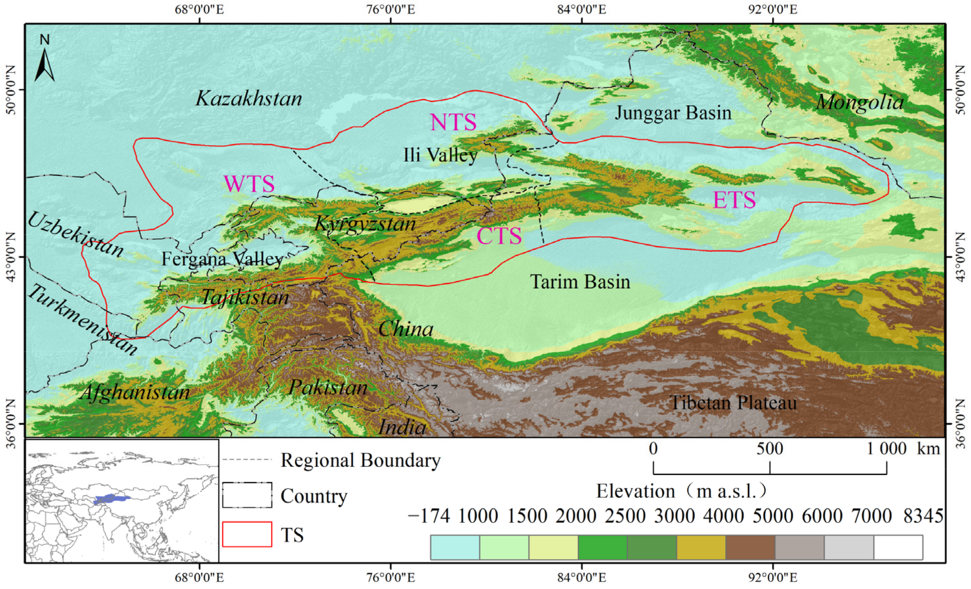
2.1. Study Area

As the largest mountain system in Central Asia, the TS stretches approximately 2500 km long and 250–350 km wide within 38°–47° N and 67°–95° E, spanning regions from Uzbekistan to Kyrgyzstan, and from southeastern Kazakhstan to Xinjiang of China (Figure 1) [48]. The TS is bordered by the Junggar Basin to the north and the Tarim Basin to the south. The major peaks in the TS stand from about 4000 to 6000 m above sea level—with the highest peak, Thomuer, at 7439 m, and the second highest peak, Khan Tengri, at 6995 m—and make up an important water tower in this in semiarid region [49]. The TS has abundant precipitation due to westerly circulation and unique topography, exhibiting heavily glaciated and snow-covered regions; annual precipitation in areas with altitude greater than 2000 m mostly exceeds 500 mm and can even reach more than 2000 mm; there are 15,953 glaciers with a total area of 15,416 km2 [26,50,51]. Based on individual mountain ranges, drainage, and climate features, the TS are geographically divided into four regions [1,26,28,52]: the Western Tienshan Mountains (WTS), the Northern Tienshan Mountains (NTS), the Central Tienshan Mountains (CTS), and the Eastern Tienshan Mountains (ETS) (Figure 1). The climate characteristics and cryosphere change show obvious differences in these four subregions [26,48,49,52]. The total area of the study area is 135.5 × 10⁴ km2; and the areas of these subregions account for 13.9% (CTS), 34.7% (WTS), 20.3% (NTS), and 31.1% (ETS), respectively (Figure 1).

2.2. Data

2.2.1. MODIS Fractional Snow Cover (FSC) Data

In this study, the MOD10A1 data for 2001–2019 distributed by the National Snow and Ice Data Center (NSIDC) [53] are utilized. There are MOD10A1 data of two versions (Collection 5 and Collection 6) through the NSIDC platform. The MOD10A1 C5 for 2001–2016 and MOD10A1 C6 for 2017–2019 are used in our work. MOD10A1 C5 provides both binary snow cover (the pixels are either snow or no-snow) and fractional snow cover (FSC) [33]. The MODIS FSC mapping algorithm, developed by Salomonson and Appel [54], is based on a statistical-linear relationship developed between the normalized-difference snow index (NDSI) from MODIS and the true subpixel fraction of snow cover as determined using Landsat scenes. Evaluation studies have demonstrated that MODIS FSC data are highly accurate (mean absolute error less than 0.1) [38,39,54,55].
FSC data are no longer provided in the MOD10A1 C6, therefore, for example, the NDSI_Snow_Cover data is used instead. In order to keep the data consistent in this study, the FSC data was obtained based the C6 NDSI_Snow_Cover product using the linear regression method [56,57]. The FSC calculation formula for MOD10A1 C6 is as follows:
FCSMOD= (−0.01 + (1.45× NDSI)) × 100
The original MOD10A1 FSC data has a sinusoidal projection, which is mosaiced and resampled from the original 463.3 m pixel size to 500 m, and converted to a WGS84-UTM geographical projection using the MODIS reprojection tool (MRT). The final mosaiced images are converted to GeoTIFF file format.

2.2.2. Meteorological Data

The ERA reanalysis, from the European Center for Medium-Range Weather Forecasts (ECMWF), is produced with a sequential data assimilation scheme, advancing forward in time by using 12-hourly analysis cycles [58,59]. The meteorological data in the TS from 2001 to 2019 are derived from the most recently released fifth generation of ECMWF reanalysis, ERA5. ERA5 reanalysis extends back to 1979 and provides hourly data at a high resolution (0.25 degree ~ 31 km). To facilitate many climate applications, the monthly-mean averages have been calculated as well in the datasets of “ERA5 monthly averaged data on single levels from 1979 to present” [60]. This dataset has been regridded to a regular lat-lon grid of 0.25 degrees for the reanalysis. To survey the linkages between SLA changes and climate variations, the monthly temperature, precipitation, and surface net solar radiation data in the TS from 2001 to 2019 are extracted from this dataset.

2.2.3. Other Data

The Shuttle Radar Topography Mission (SRTM) is a set of freely available global digital elevation data covering over 80% of the globe. In this study, the data are available at 1 arc-second (∼30 m) resolution, with vertical accuracy reported as less than 16 m from the U.S. The grid size of the DEM is resampled to 500 m in order to remain consistent with the MODIS snowline pixels, and 500 m DEM is used to derive the SLA and calculate the slope gradient and aspect within the study area.
In order to facilitate the analysis of SLA dynamics and the extraction of ERA5 meteorological grid data (about 31 km spatial resolution), the entire study area is divided into 1715 grids (i.e., the numbers of grids for the NTS, CTS, ETS, and WTS are 350, 240, 526, and 599, respectively) with a cell size of 30 km. Eighty-two Landsat Operational Land Imager (OLI) images (Table 1) covering the four grids for validation are used as reference data for the SLA evaluation. The selection of these Landsat images primarily depends on cloud cover.

2.3. Methodology

Taking the 130th day of 2016 as an example, the process of SLA determination from MODIS FSC products is presented in Figure 2, including the cloud removal from MODIS FSC data, extracting the largest lake mask, and determination of snowline and SLA.

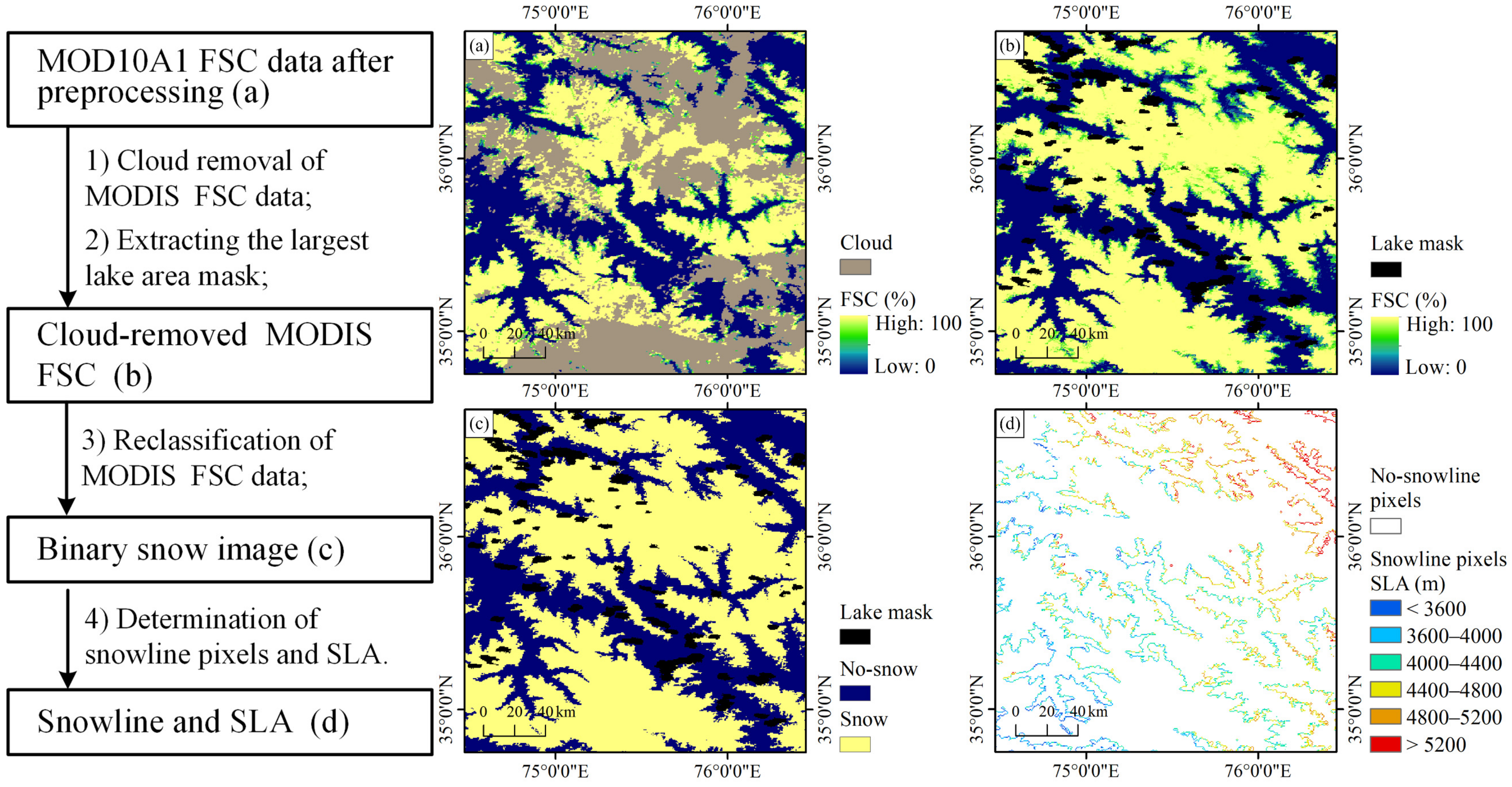
2.3.1. Cloud Removal from MODIS FSC Data

The extensive cloud cover over snow-covered region is a critical issue that greatly limits the applications of the MODIS snow cover product to monitor the snow cover and snowline [33,38]. A validation study of MODIS snow cover images over the Tibetan Plateau found that about 47.3% of the areas were cloud covered [39]. Previous studies suggest that the FSC maps more accurately represent the gradual changes of snow cover in each pixel than the binary snow cover maps [33,54], thus the use of the FSC data could be better for the removal of the cloud cover by temporal filtering [39]. Following the cloud removal method for MODIS FSC products developed by Tang et al. [39], the daily cloud-removed FSC data in the study area are produced from 2001 to 2019. The cloud removal algorithm is based on the cubic spline interpolation algorithm (temporal filtering). Details on the cubic spline interpolation cloud removal method and the relevant accuracy evaluation strategies can be found in the works of Tang et al. [39], and the method is also similar in principle to that proposed by Dozier et al. [61]. From the applications of the cloud removal method in the Tibetan Plateau and the TS [30,39,62,63], the cloud removal method is efficient in retrieving the FSC information of the cloud-covered pixels in these areas, with the overall mean absolute error less than 0.1. There is a high consistency between MODIS-derived snow-covered days (SCD) and the in-situ observed SCD, with a mean consistency over 85%, and a mean absolute error of less than 4.2 days [30,39]. The higher consistency between MODIS-derived SCD and in situ SCD indicates that the cloud-removed MODIS FSC data have a high accuracy to monitor the snowline in the TS.

2.3.2. Extracting the Largest Lake Area Mask

There are around 1667 lakes in the TS, with total area 96.5 ± 14.2 km2 of the TS. The number of lakes along with the total lake area have been in a state of continuous increase in the past few decades [52]. In general, the inland water bodies have been automatically identified (the code is 237) in MODIS snow products. However, due to the existence of lakes, it is easy to misclassify snow in the cold season. Seasonally frozen lakes (lake ice) are often erroneously identified as snow-covered areas due to the similar spectral characteristics of snow and ice. In such cases, the low-elevation lake boundaries are extracted as snowline, which causes incorrect results.
To solve this problem, the largest lake area mask (Figure 2b) is produced from a composite of 19 years (2001–2019) of MOD10A1 FSC data (Figure 2a) to eliminate the influence of lake ice. The inland water that is identified in each pixel in the 19 years of MOD10A1 FSC data for more than one day is taken as the lake pixel. Simultaneously, some snowline pixels located in the largest lake area mask were eliminated in the process of snowline extracting. Figure 3 presents the spatial distribution of the largest extracted lake area mask. Meanwhile the mean SCD is used as the base map, which is derived from the cloud-removed daily MODIS FSC datasets during 2001–2019.

2.3.3. Determination of Snowline and SLA

The determination of snow cover through the availability of the cloud-removed MODIS FSC data is an important step. The snowline is theoretically equivalent to the snow cover outline, which is at the edge of the snow-covered areas. A binary map of snow is tuned to classify a pixel as snow if its coverage is greater than 50% (i.e., FSC ≥ 50%) and snow-free otherwise (Figure 2c). Thus, the pixels at the edge of the snow-covered areas (snowline pixels) are extracted; for each snow-covered pixel, if there is one or more of its surrounding pixels that are no-snow and the pixel is not located in the largest lake area mask, we marked it as a snowline pixel (Figure 2d).
Once the snowline pixels have been marked, the SLA (Figure 2d) can be determined by overlaying the snowline image on the 500 m DEM. Then the determination of SLA for every 30 km grid was carried out by means of the SLA of 500 m snowline pixels.

2.3.4. SLA Dynamics Analysis

In this study, the application of the Mann–Kendall (M–K) test is to assess the temporal significance of trends in meteorological factors and SLA from 2001 to 2019 on a grid-by-grid basis. The M–K test is a nonparametric method of monotonic trends that has successfully been applied to detect trends in a time series [64,65,66,67]. The statistical significance of temporal trends is assumed by Z value, and the significance of the trends is evaluated with a confidence level of p < 0.05 [68]. Sen’s slope is used to estimate the magnitude of trends in meteorological factors and SLA from 2001 to 2019 in this study. The advantage of Sen’s slope is to deal with data of non-normal distribution, and it is used instead of a linear regression because it limits the influence that the outliers have on the slope [69,70]. In addition, correlation analysis was performed to analyze the relationship between SLA, temperature, precipitation, and solar radiation on a grid-by-grid basis.

3. Results

3.1. Comparison of SLA Derived from MODIS FSC and Landsat OLI Images

To evaluate the method, we compared the SLA of four grids extracted from Landsat images (Table 1) with the extraction results from MODIS. The process of SLA determination for a grid from Landsat images can be sketched as follows. First, Landsat images are classified as snow or non-snow using the SNOWMAP approach [71]. Then, the boundaries (snowline pixels) between snow cover and land are extracted. Lastly, the SLA of the grid is determined as the average elevation of the multiple snowline pixels by combination with the 30 m SRTM DEM. The mean absolute error and root mean square error are employed to evaluate the reliability of the MODIS-derived SLA (Table 2). In the four validation grids, the mean absolute error of MODIS-derived SLA compared with the Landsat-derived values is between 7.8 and 14.6 m, and the root mean square error is between 9.7 and 16.7 m. We believe that the MODIS-derived SLA with such accuracy in the 30 km grids can be applied to investigating the spatiotemporal patterns of SLA in the TS.

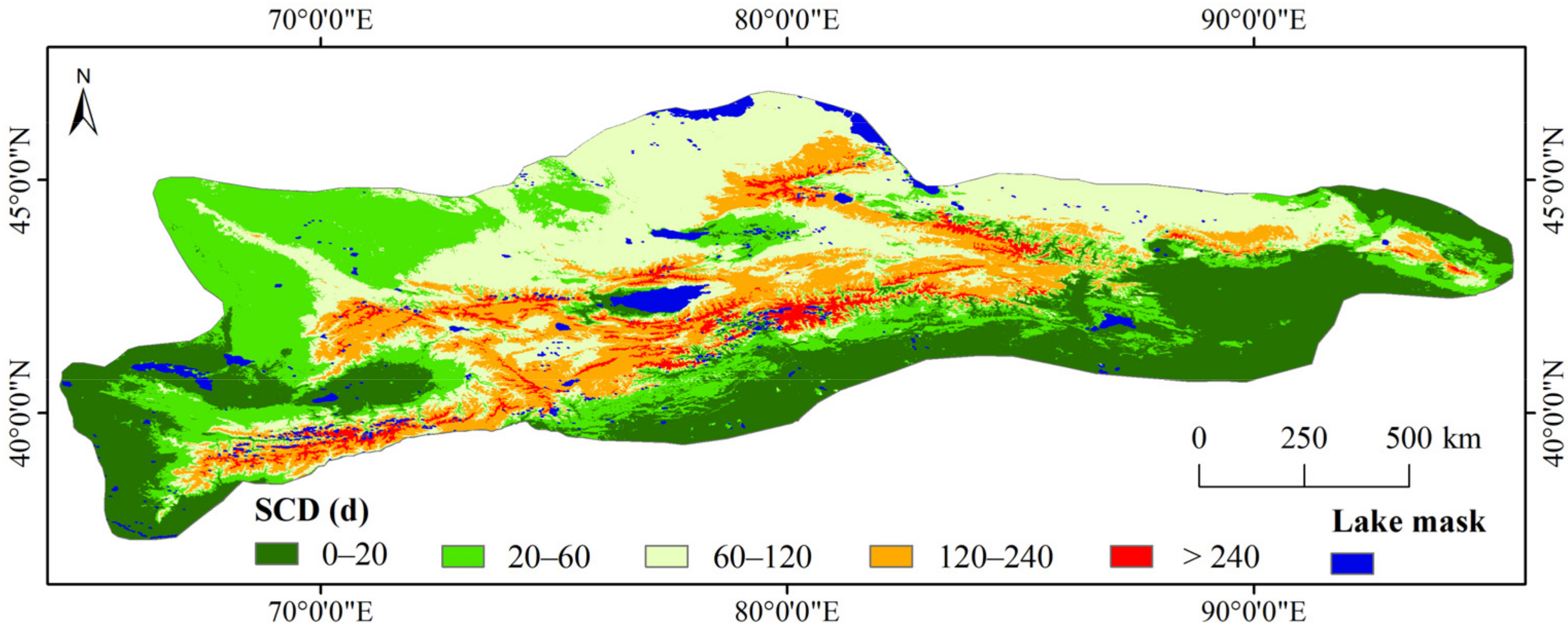
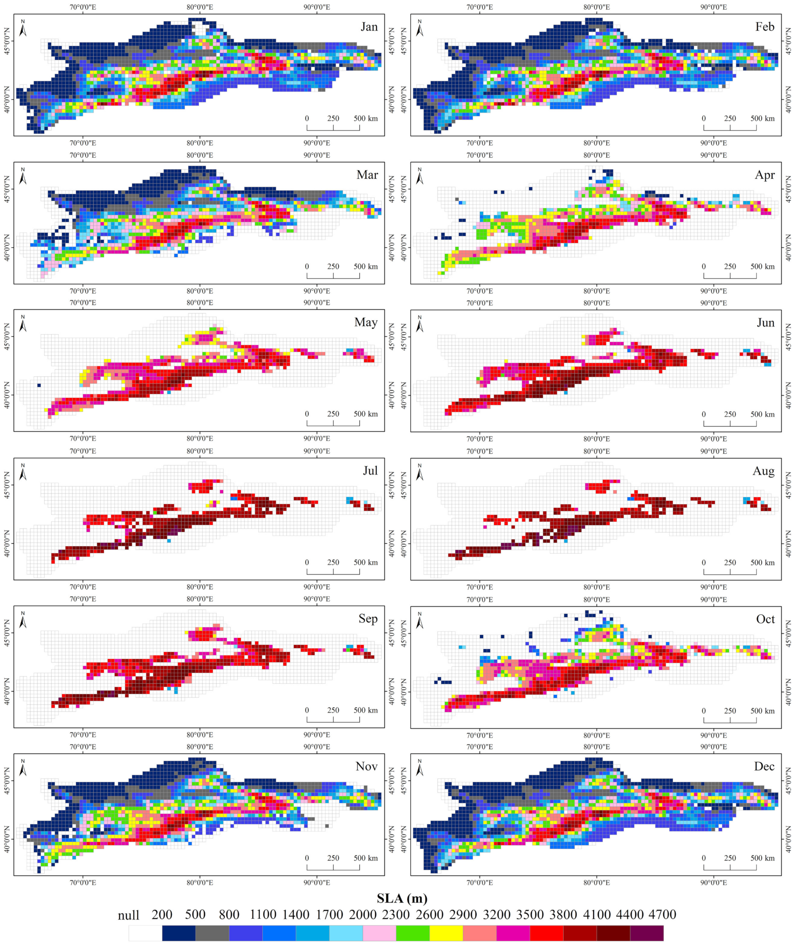
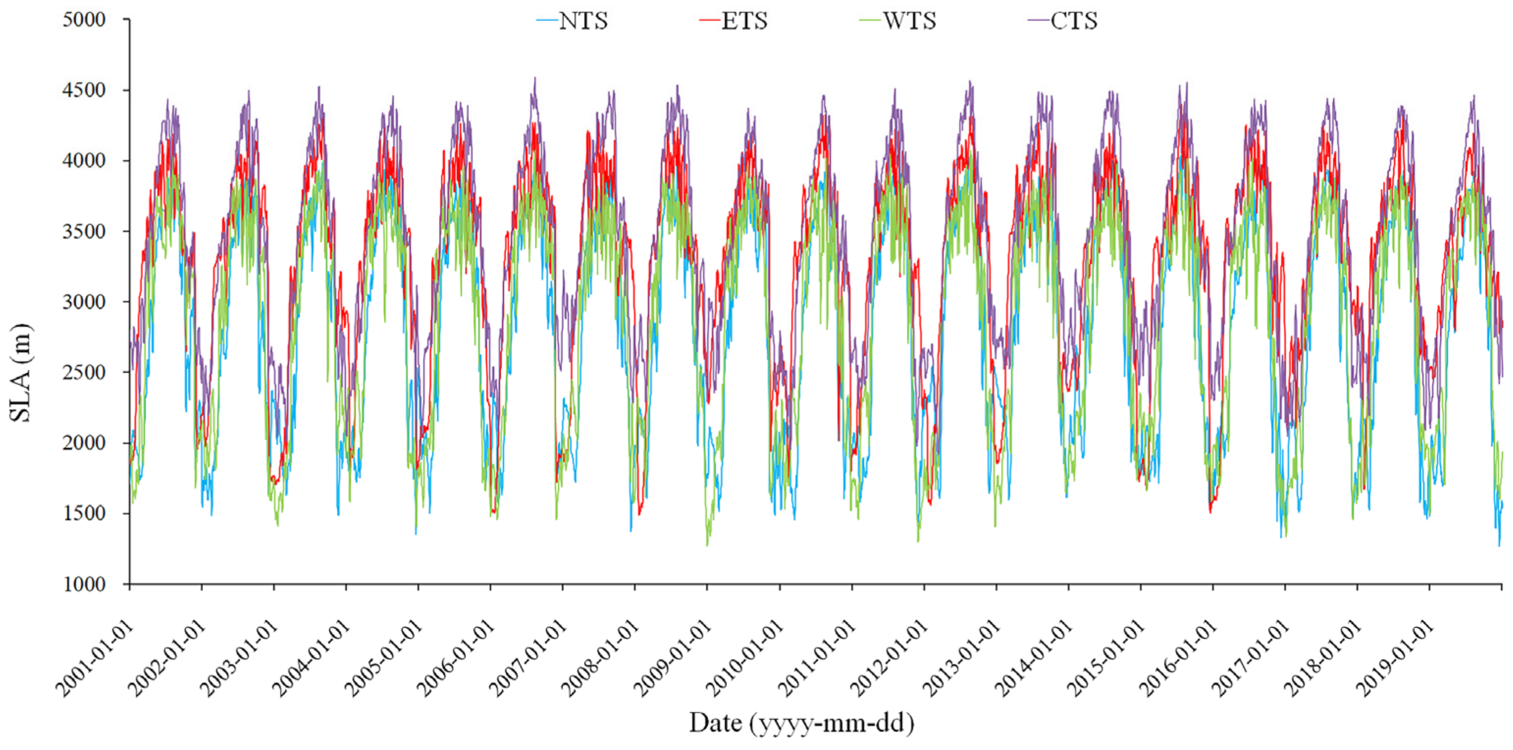
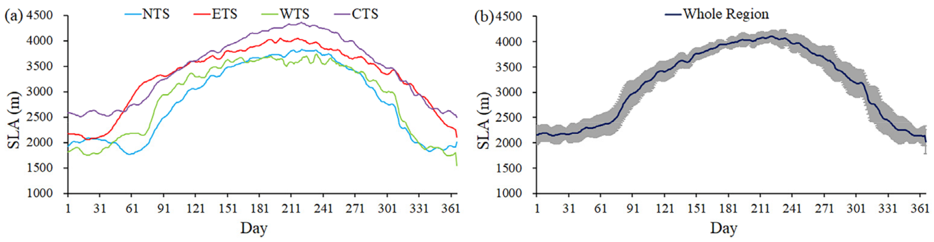
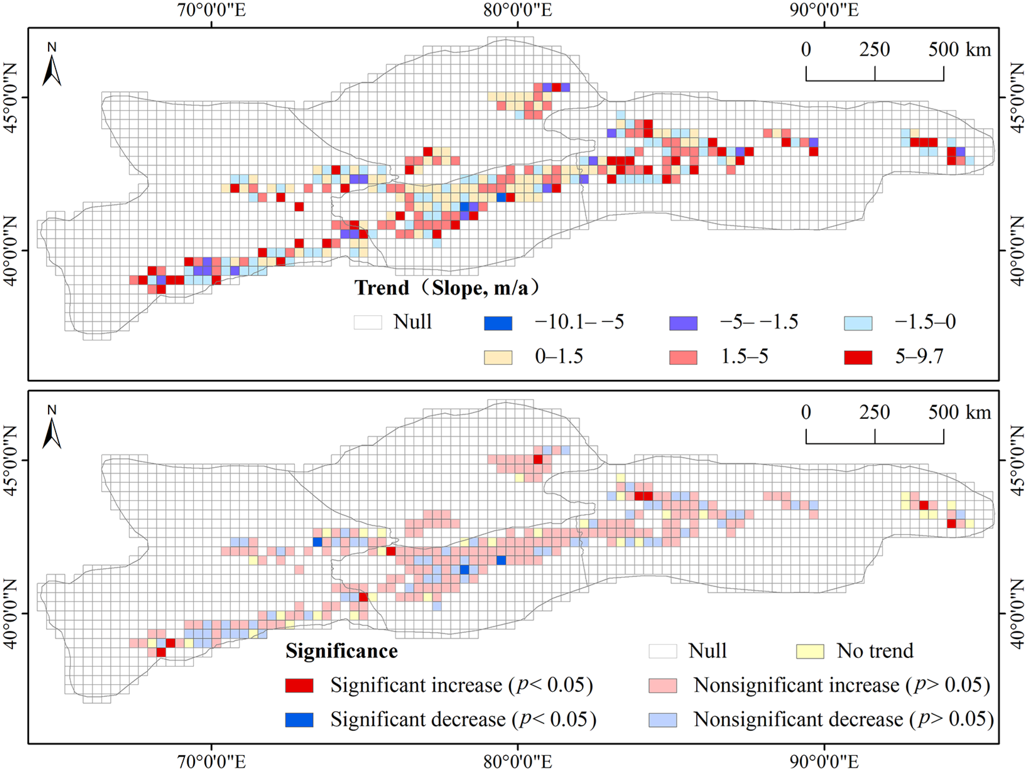
3.2. Spatiotemporal Patterns of SLA

Figure 4 presents the spatial pattern of multiyear (2001–2019) mean SLA for different months over the TS. The spatial distribution of the SLA over the entire TS exhibits a large spatial heterogeneity and corresponds well with the distribution of snow duration (SCD in Figure 3). Apparently, in the peripheral mountainous area, SLA is relatively low. By contrast, SLA is high in the vast interior area (especially in the CTS). Furthermore, Figure 5 and Figure 6 show the time series of SLA for the four subregions from 2001 to 2019, and the annual cycles of SLA over the entire TS and the four subregions, respectively. Strong seasonal variations in SLA are found over the whole area of the TS (Figure 4, Figure 5 and Figure 6). The seasonal variations range of SLA is from about 2000 to 4100 m. The SLA from the end of November to early March of the following year is lower than 2400 m, with relatively large standard deviations reflecting the high interannual variability, whereas in the June–September period, the average SLA is greater than 3900 m and with a relatively small interannual variability (Figure 6b). Apparently, the SLA over the TS progressively increases, beginning in March due to the snowpack ablation, and reaches the highest in August. A steady decrease of SLA begins in September along with the accumulation of snow, and reaches relatively low (average SLA of 2209 m) in winter (Figure 6b).
However, for different subregions, the differences in the seasonal fluctuations of SLA exhibit distinct climatological characteristics (Figure 6a). The NTS is situated under the strong influence of the Siberian anticyclonic circulation, which brings precipitation mainly in the form of snowfall in the cold season; simultaneously, it is also influenced by frontal cyclonic circulation and northern jet stream, which bring considerable precipitation even in the cold season [49]. As a result, the lowest SLAs occur in the NTS (Figure 6a). In winter, the WTS is weakly influenced by the Siberian anticyclonic circulation, and the southwest cyclonic circulation is moderate in winter, bringing in warm moist air and maximum precipitation; however, winter precipitation is relatively rare for the CTS and ETS [30,49]. This may explain why the SLA in the WTS is relatively lower than that in the CTS and ETS (Figure 6a). The CTS has high mountains, so the transport of water vapor from the Atlantic is blocked. The CTS is also adjacent to the Taklamakan Desert, and has dry air, unlike the other subregions of the TS. In addition, the topographic-altitude-controlled spatial pattern of the SLA could be ascribed to the mass elevation effect, which is essentially the result of the thermodynamic effect of mountain masses and has been recognized as a significant contributor to the vertical distribution of mountain snowline and timberline [72,73]. Thus, SLA in the CTS is dramatically higher than the other regions.
To explore the variations of SLA in detail, the slope (Sen’s slope) of the trend in SLA for the whole study area and the counts of SLA grids at the 5% significance level were calculated on a grid-by-grid and month-by-month basis during the period 2001–2019 (Table 3 and Table 4). Besides, the change trend (slope) of SLA and its significance level in August for the 19 years are depicted in Figure 7 as an example. On the whole (excluding the null value grids), the SLA over the entire TS shows a rising trend in August (the average slope of the grids is 1.95 m/a), although a large number of grids (53.5%) are characterized by weak trends in SLA (−1.5 < slope < 1.5 m/a) (Figure 7). Overall, 58.1% of the grids are increased (0 < slope < 9.7 m/a), but only 28% of the grids are characterized by decreasing trends (−10.1 < slope < 0 m/a). For the different subregions, the average slopes of NTS, ETS, WTS, and CTS are 1.36 m/a, 2.79 m/a, 2.08 m/a, and 1.29 m/a, respectively. As shown in Table 3 and Table 4, the SLA over the entire TS from 2001 to 2019 generally displays an increasing trend. In particular, the increasing trends are notable both at the start of the melt season SLA (March and April) and the end of melt season SLA (July and August) for the four subregions. Despite the number of significantly decreased SLA grids (93) exceeding the number of the significantly increased grids (10), the SLA in November over the entire TS is rising. A slight decrease of the SLA in June is found for the entire TS (−1.17 m/a) during 2001–2019, with most of the decrease stemming from the ETS.

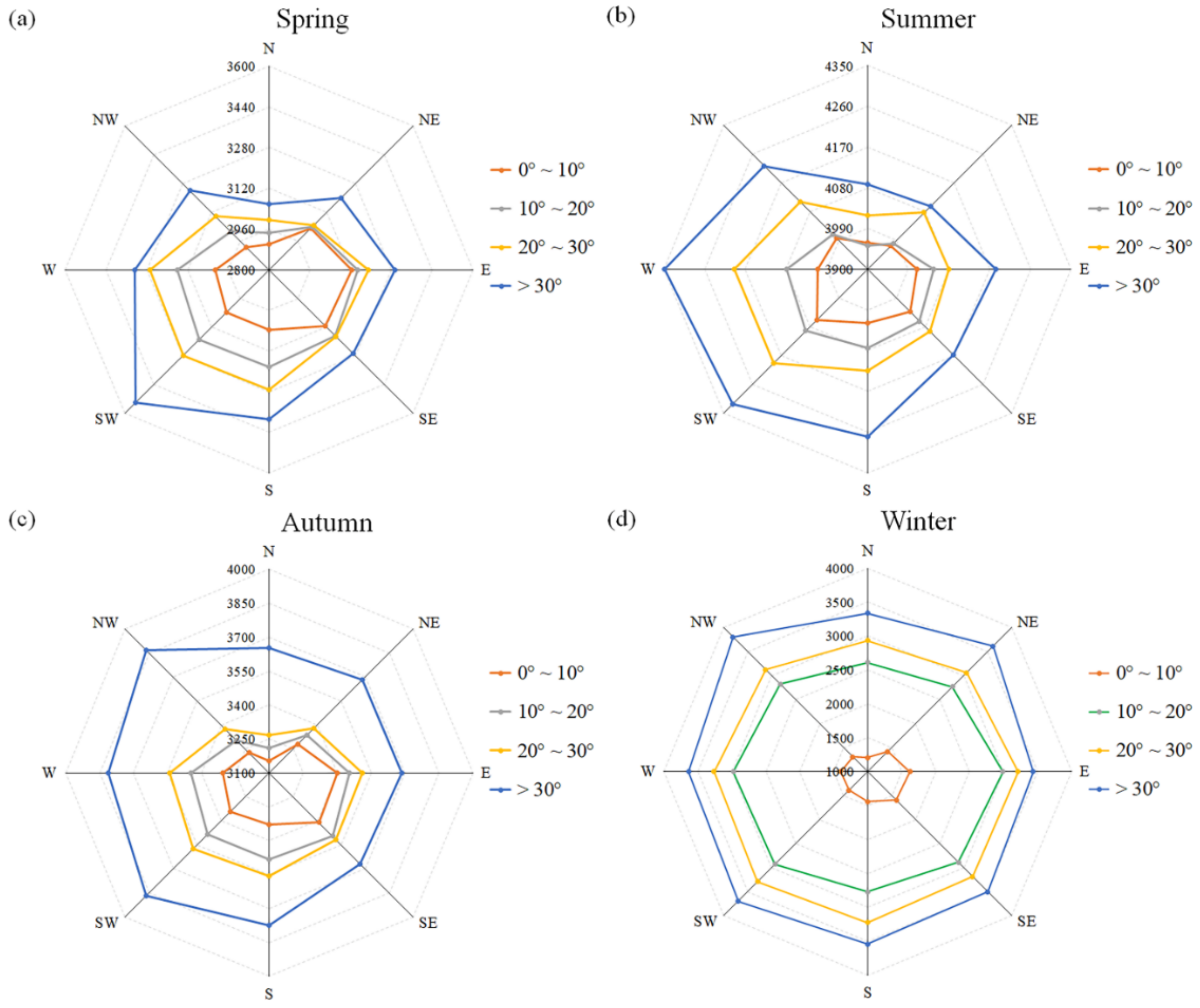
3.3. The Influences of Topographic Factors on SLA

In high mountain regions, like the TS, SLAs in areas with similar climatic conditions might respond differently given their different and complex topographies. In order to investigate the variation characteristic of SLA in different topographic conditions, the aspect and slope gradient calculated by DEM are used in this study. The aspect of the TS is set as the eight ranges: north (0°–22.5°, 337.5°–360°), northeast (22.5°–67.5°), east (67.5°–112.5°), southeast (112.5°–157.5°), south (157.5°–202.5°), southwest (202.5°–247.5°), west (247.5°–292.5°), and northwest (292.5°–337.5°). Likewise, the slope gradient is divided into four ranges (0°–10°, 10°–20°, 20°–30°, and >30°).
From the SLA over the TS relative to different slope gradients located in four aspect ranges (Figure 8), it is evident that the SLA increases with the steeper slope gradient. As the slope gradient gradually increases, the SLA changes greatly. SLA within the slope gradient of 0°–10° is considerably lower than other slope gradients in winter. In addition, areas having a southerly aspect receive more solar radiation than the north, resulting in more heat absorption and higher SLA (Figure 8). In contrast, SLAs in the Himalayan region are lower on the southerly aspect because of the influence of two atmospheric circulations: the Indian Ocean and the summer southwest monsoon [36]. The two circulation systems, combined with the huge topographic landform, exert climatic controls on the distribution of SLA in the Himalayan region. Due to significant shielding of water vapor transport by high topography as atmospheric travels north across the region, the southern aspects are enriched and the northerly aspect depleted in their abundance of precipitation.

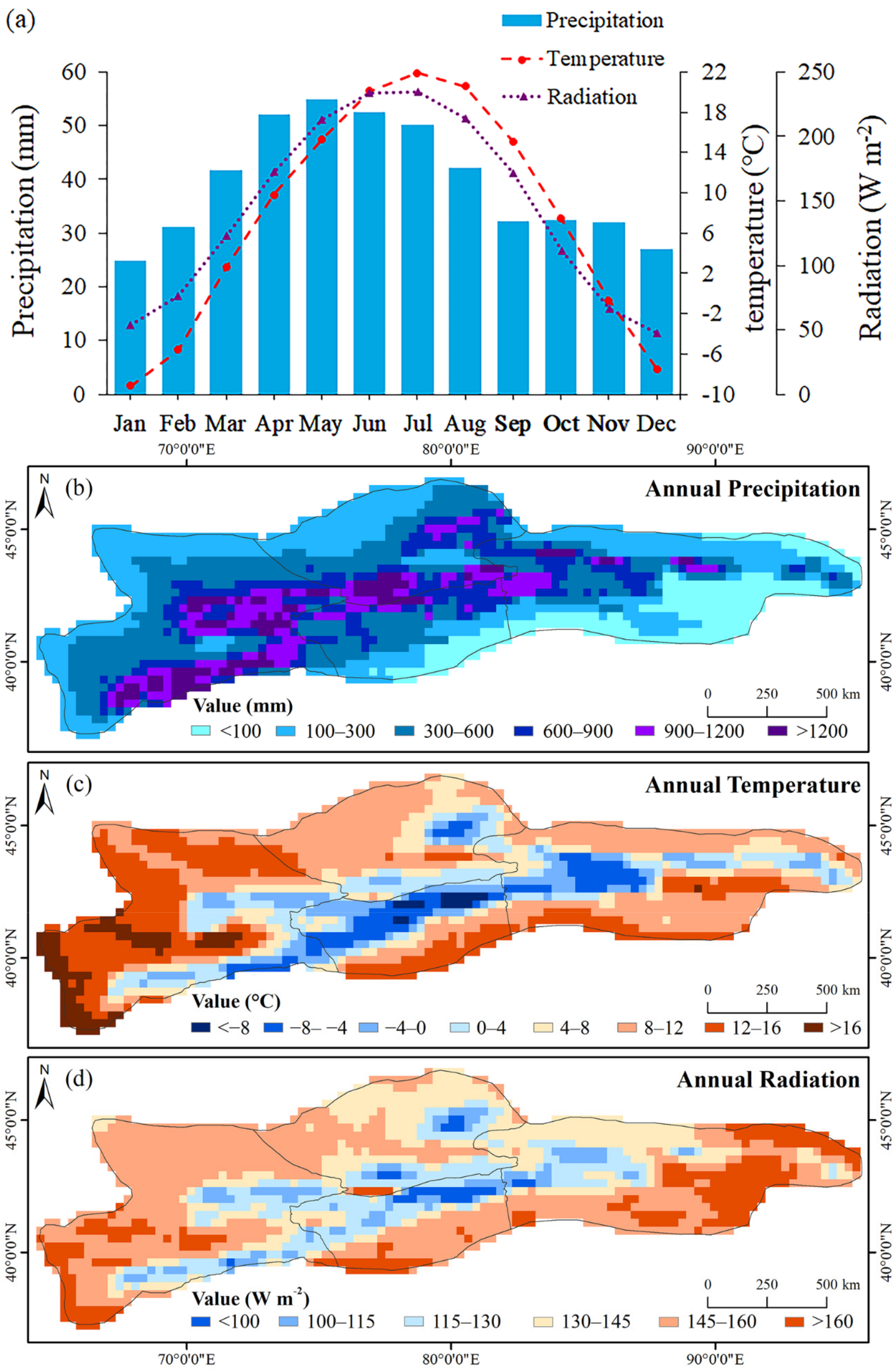
3.4. Spatiotemporal Characteristics of Meteorological Factors Over the TS

Monthly distribution of precipitation, temperature, and solar radiation in the TS during 2001–2019 shows obvious seasonal variations (Figure 9). The annual mean precipitation across the TS is 469.4 mm, which is concentrated between April and July; the annual mean temperature is 7.5 ℃; and the annual mean radiation is 143.1 W m−2 (Figure 9a). The temperature and solar radiation tend to be remarkably consistent in their changes during the year. Spatial distributions of the precipitation, temperature, and solar radiation are shown in Figure 9b–d. The WTS and NTS have the greater annual precipitation, and are characterized by a relatively humid climate, while the CTS and ETS have a typical continental climate. Besides, areas peripheral to the TS are characterized by less precipitation. In contrast, the temperature and solar radiation are low in the central region and high in the marginal region.

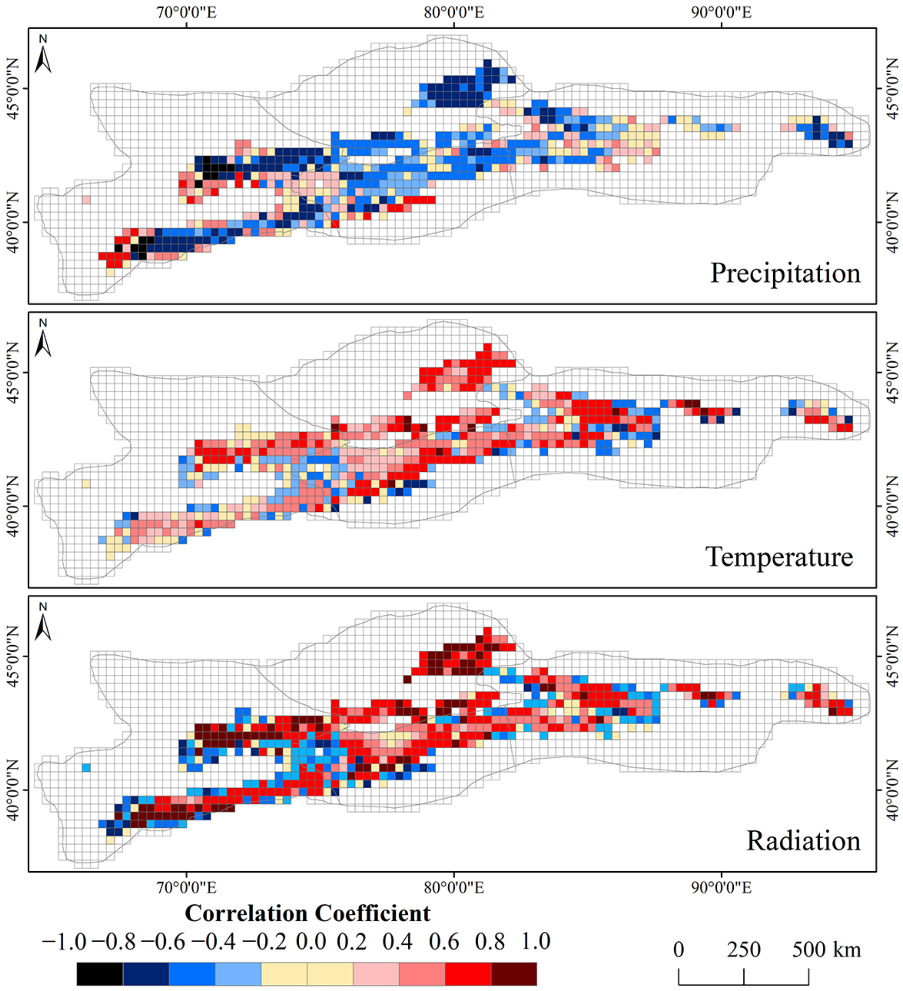
3.5. The Influences of Meteorological Factors on SLA

To explore possible mechanisms for SLA changes of the TS, we examined the correlation between SLA and the variations of three important meteorological factors (temperature, precipitation, and solar radiation) by correlation analysis. In this study, the monthly averaged ERA5 climate reanalysis data were selected to investigate the relationship between SLA, temperature, precipitation, and solar radiation at monthly scales. Taking October as an example, the Pearson correlation coefficients between SLA, temperature, precipitation, and solar radiation during 2001–2019 are calculated on a grid-by-grid basis (Figure 10). As can be seen from Figure 10, the correlation between SLA, temperature, and solar radiation shows obvious consistency. The SLA increases with the increased temperature and radiation in most areas of the TS (particularly in the WTS and CTS). It is evident that the SLA decreases with increased precipitation, except for a small part of the ETS (Figure 10). Additionally, correlation coefficients between SLA, temperature, and solar radiation vary in different regions and months (Table 5). In March–June, it shows a significant correlation between SLA, temperature, and solar radiation in the entire TS, while the correlation between SLA and precipitation is insignificant. From September to November, these meteorological factors have a great influence on SLA changes, with solar radiation being the dominant one. In the winter period (i.e., from December to February of the following year), the SLA shows no obvious correlation with temperature, precipitation, or solar radiation. Because of the temperature being well below freezing in winter, there is little temperature-related snow melting. The increased sublimation of the snow may cause the reduction of winter snow at high altitudes where it is frequently accompanied by high winds. More than half of the snow mass in the Tibetan plateau is lost by sublimation in winter [74].

4. Discussion

The TS is the main water source and ecological barrier of Central Asia, with unique climatic and hydrological conditions. Based on MODIS snow cover products, this study extracts spatiotemporal continuous SLA of the entire TS for 19 years. The uncertainty of the MODIS-derived SLA may come from the following: (1) the errors that occurred due to the pixel size of the remote sensing images, slope, and aspect of the terrain, affecting the accuracy of the georeferencing and the quality of the DEM [75,76]; or (2) the errors that occurred in the MODIS FSC mapping algorithm [38,77] and cloud removal method [39], although the MODIS SCD threshold is calibrated in this method. For MODIS FSC mapping, Masson et al. has shown that NDSI linear regression produced better results when used alongside atmospheric and topographic correction [78]; a new linear regression model could be defined if a large series of validated and very accurate ground truth data were to be established. In addition, the linear spectral unmixing approach is a more reliable method for estimating snow cover fraction, and tends to produce more stable results than the NDSI linear regression method [78]. Therefore, future research should examine the SLA method presented here with the MODSCAG and MODImLAB approaches [79,80]. Given the high resolution, the Landsat and Sentinel-2 images are suitable for high-resolution SLA extraction. However, the cloud cover and longer revisit period greatly limit their ability. Google Earth Engine (GEE) is a cloud-based platform that makes it easy to access high-performance computing resources for processing very large geospatial datasets [81]. The GEE platform integrates the Landsat and Sentinel-2 images from over the last few decades, which can be accessed and processed by the Earth Engine application programming interface (API). Therefore, the GEE platform provides a possible method for SLA extraction in a continuous time and space for a large-scale area.
The MODIS-derived SLA method and gridded approach in this study can be efficiently applied to SLA extraction for other large-scale areas. For a catchment scale, however, the regional snowline elevation can be better obtained by the method developed by Krajčí et al. in the case of cloud cover (<70%) [15]. However, this method must estimate an elevation (i.e., the regional snowline elevation) where the number of snow-covered pixels below and the number of snow-free pixels above are minimized, and only obtains one SLA value for the entire basin [15]. If we want to estimate SLA dynamics and their long-term trends at the catchment level, the recent study gives an available method of random forest regression [82] combining high resolution satellite imagery and climate reanalysis data.
Under the background of global warming, and the state of high variability in temperature of the TS since 1997 [45], the cryosphere of the TS has been changing rapidly [28,83,84,85]. Like many glaciers worldwide, the glaciers in the TS have generally been losing mass over the past decades [28,86,87]. In this work, we find the SLA in the TS generally shows a rising trend in the 19 years (Table 3 and Table 4). This increasing trend is especially significant at the end of melting season (July and August), and especially in August, with average slopes of NTS (1.36 m/a), ETS (2.79 m/a), WTS (2.08 m/a), and CTS (1.29 m/a). These rising trends of SLA at the end of melting season indicate a decrease in the annual mass balance of glaciers across the 19 years. Glaciers in the TS are generally losing mass (i.e. average annual mass balance is already negative) [28,85]. These results are consistent with the conclusions drawn from previous studies on the relationship between the glacier mass balance and SLA at the end of melting season [23,25,88]. It would be more beneficial to reconstruct the annual mass balance time series if higher resolution data could be used for estimating spatial and temporal continuous SLA over a large-scale area.
Due to the specific geographical location and climatic conditions, the snow cover and mountain glaciers in the TS are very vulnerable to climate change. Our results show a strong correlation between SLA, temperature, precipitation, and solar radiation (Figure 10), although the absolute values of the correlation coefficients vary due to the different subregions. That is, the SLA increases with increased temperature/radiation and decreased precipitation. Solar radiation is the dominant climatic factor affecting the changes of SLA in the TS (Table 5). Due to the reduction in surface albedo caused by the decrease in glacier and snow coverage, more solar radiation will be absorbed, and will then amplify cryosphere warming, further intensifying ablation and snowmelt [89,90]. Nevertheless, the effect of climate change on SLA is very complex. The 19 years of available MODIS information is insufficient for definitive conclusions about climate change. Longer time series of data need to be examined in further studies to obtain some more definitive conclusions about temporal trends of SLA and their relationship with climate change.

5. Conclusions

In this study, a large-scale SLA investigation methodology is developed using the cloud-removed MODIS FSC products (MOD10A1). The 500 m resolution of a daily SLA dataset is generated over the TS for the period 2001–2019. The spatiotemporal patterns of SLA over the entire TS during 2001–2019 are investigated using the gridded approach, with specific attention to the four subregions. We also explore the potential influence of topographic factors (slope gradient and aspect) on SLA and the correlation between SLA and meteorological factors (temperature, precipitation, and solar radiation) on a grid-by-grid and month-by-month basis. The main findings are summarized as follows:
(1) The large-scale SLA monitoring method is efficient in monitoring the spatiotemporal patterns of the SLA in the TS. Compared with the Landsat-derived SLA of the four validation grids (30 km), the mean absolute error of MODIS-derived SLA is between 7.8 and 14.6 m, and the root mean square error is between 9.7 and 16.7 m.
(2) Our results show strong seasonal fluctuations of SLA over the TS from 2001 to 2019, ranging from about 2000 (in late December) to 4100 m (in early August). The distribution of SLA over the TS shows a large spatial heterogeneity due to complex topography and geomorphology. The SLA increases with the steeper slope gradient. The SLA of the northerly aspect is generally less than that of the south, due to receiving more solar radiation.
(3) The SLA over the entire TS from 2001 to 2019 shows a rising trend. Except for a slight decrease in June, the SLA increased in all other months, especially at the start of the melting season (March and April) and the end of the melting season (July and August). The SLA increases with increased temperature/radiation in the TS (particularly in the WTS and CTS) and decreases with increased precipitation. Solar radiation is the dominant climatic factor leading the SLA dynamics, and temperature has a greater influence on SLA than precipitation. This study could enrich the understanding of the response of snow cover dynamics to climate, and provide scientific support for eco-environment sustainable management in the high mountain region. If global warming continues, the melting of snow and peak runoff in the TS will increase. The early snowmelt may lead to a decrease in summer flow, which in turn changes the flow regimes and water availability, thereby affecting the ecosystem, agriculture, and water resources in the densely populated downstream areas.

Author Contributions

All authors contributed to the design and development of this manuscript. Conceptualization, Z.T.; methodology, G.D. and Z.T.; validation, G.D., G.H., and J.W.; formal analysis, G.D. and Z.T.; investigation, G.D. and G.H.; data curation, G.S., J.L., and J.W.; writing—original draft preparation, G.D.; writing—review and editing, G.D., Z.T., and G.H.; supervision, Z.T.; project administration, Z.T.; funding acquisition, Z.T. All authors have read and agreed to the published version of the manuscript.

Funding

This study was supported financially by the National Natural Science Foundation of China (No. 41871058), the State Key Laboratory of Cryospheric Science, Northwest Institute of Eco-Environment and Resources, Chinese Academy Sciences (No. SKLCS-OP-2020-08); the Foundation for Innovative Research Groups of the Natural Science Foundation of Hunan Province, China (No. 2020JJ1003); and the Scientific Research Foundation of Hunan Education Department, China (No. 20B227).

Institutional Review Board Statement

Not applicable.

Informed Consent Statement

Not applicable.

Data Availability Statement

Data sharing not applicable.

Acknowledgments

We would like to thank the editors and reviewers (especially Keith A. Brugger) for their helpful comments and constructive suggestions. MODIS fractional snow cover data were obtained from the National Snow and Ice Data Center (NSIDC) (https://nsidc.org/, accessed on 19 June 2020). The temperature, precipitation, and solar radiation datasets were obtained from “ERA5 monthly averaged data on single levels from 1979 to present” (https://cds.climate.copernicus.eu/cdsapp#!/search?type=dataset&text=ERA5, accessed on 19 June 2020).

Conflicts of Interest

The authors declare no conflict of interest.

References

  1. Kaur, R.; Saikumar, D.; Kulkarni, A.V.; Chaudhary, B.S. Variations in snow cover and snowline altitude in Baspa Basin. Curr. Sci. 2009, 10, 96. [Google Scholar]
  2. Brown, R.D.; Robinson, D.A. Northern Hemisphere spring snow cover variability and change over 1922–2010 including an assessment of uncertainty. Cryosphere 2011, 5, 219–229. [Google Scholar] [CrossRef] [Green Version]
  3. Ke, C.-Q.; Li, X.-C.; Xie, H.; Ma, D.-H.; Liu, X.; Kou, C. Variability in snow cover phenology in China from 1952 to 2010. Hydrol. Earth Syst. Sci. 2016, 20, 755–770. [Google Scholar] [CrossRef] [Green Version]
  4. Malmros, J.K.; Mernild, S.H.; Wilson, R.; Tagesson, T.; Fensholt, R. Snow cover and snow albedo changes in the central Andes of Chile and Argentina from daily MODIS observations (2000–2016). Remote Sens. Environ. 2018, 209, 240–252. [Google Scholar] [CrossRef] [Green Version]
  5. Wu, X.; Shen, Y.; Zhang, W.; Long, Y. Fast Warming Has Accelerated Snow Cover Loss during Spring and Summer across the Northern Hemisphere over the Past 52 Years (1967–2018). Atmosphere 2020, 11, 728. [Google Scholar] [CrossRef]
  6. Yang, Y.; Wu, X.-J.; Liu, S.-W.; Xiao, C.-D.; Wang, X. Valuating service loss of snow cover in Irtysh River Basin. Adv. Clim. Chang. Res. 2019, 10, 109–114. [Google Scholar] [CrossRef]
  7. Wu, X.; Wang, X.; Liu, S.; Yang, Y.; Xu, G.; Xu, Y.; Jiang, T.; Xiao, C. Snow cover loss compounding the future economic vulnerability of western China. Sci. Total. Environ. 2021, 755, 143025. [Google Scholar] [CrossRef]
  8. Seidel, K.; Ehrler, C.; Martinec, J. Derivation of Statistical Snow Line from High Resolution Snow Cover Mapping. In Remote Sensing of Land Ice and Snow; EARSeL Workshop: Münster, Germany, 1997; pp. 31–36. [Google Scholar]
  9. Licker, M.D. Dictionary of Earth Science; McGraw-Hill: New York, NY, USA, 2003. [Google Scholar]
  10. Kaur, R.; Kulkarni, A.V.; Chaudhary, B. Using RESOURCESAT-1 data for determination of snow cover and snowline altitude, Baspa Basin, India. Ann. Glaciol. 2010, 51, 9–13. [Google Scholar] [CrossRef] [Green Version]
  11. Wunderle, S.; Droz, M.; Kleindienst, H. Spatial and temporal analysis of the snow line in the alps: Based on NOAA-AVHRR data. Geogr. Helv. 2002, 57, 170–183. [Google Scholar] [CrossRef] [Green Version]
  12. Hantel, M.; Maurer, C. The median winter snowline in the Alps. Meteorol. Z. 2011, 20, 267–276. [Google Scholar] [CrossRef]
  13. Deng, Y.; Xie, Z.; Qin, J.; Wang, X.; Qiaoyuan, L.I. The Field of Equilibrium Line Altitude in the Ganga-Yarlung Zangbo Rivers System: Establishment and Its Environmental Significance. J. Geogr. Sci. 2006, 28, 865–872. [Google Scholar]
  14. Girona-Mata, M.; Miles, E.S.; Ragettli, S.; Pellicciotti, F. High-Resolution Snowline Delineation from Landsat Imagery to Infer Snow Cover Controls in a Himalayan Catchment. Water Resour. Res. 2019, 55, 6754–6772. [Google Scholar] [CrossRef] [Green Version]
  15. Krajčí, P.; Holko, L.; Perdigão, R.A.; Parajka, J. Estimation of regional snowline elevation (RSLE) from MODIS images for seasonally snow covered mountain basins. J. Hydrol. 2014, 519, 1769–1778. [Google Scholar] [CrossRef]
  16. Holzer, T.; Baumgartner, M.; Apfl, G. Monitoring Swiss Alpine Snow Cover Variations Using Digital NOAA-AVHRR Data. In Proceedings of the 1995 International Geoscience and Remote Sensing Symposium, IGARSS ’95. Quantitative Remote Sensing for Science and Applications, Firenze, Italy, 10–14 July 1995; Volume 3, pp. 1765–1767. [Google Scholar]
  17. Zappa, M. Objective quantitative spatial verification of distributed snow cover simulations—an experiment for the whole of Switzerland / Vérification quantitative spatiale objective de simulations distribuées de la couche de neige—Une étude pour l’ensemble de la Suisse. Hydrol. Sci. J. 2008, 53, 179–191. [Google Scholar] [CrossRef]
  18. Gafurov, A.; Bárdossy, A. Cloud removal methodology from MODIS snow cover product. Hydrol. Earth Syst. Sci. 2009, 13, 1361–1373. [Google Scholar] [CrossRef] [Green Version]
  19. Parajka, J.; Pepe, M.; Rampini, A.; Rossi, S.; Blöschl, G. A regional snow-line method for estimating snow cover from MODIS during cloud cover. J. Hydrol. 2010, 381, 203–212. [Google Scholar] [CrossRef]
  20. Østrem, G. The transient snowline and glacier mass balance in southern British Columbia and Alberta, Canada. Geogr. Ann. Ser. A-Phys. Geogr. 1973, 55, 93–106. [Google Scholar] [CrossRef]
  21. McFadden, E.M.; Ramage, J.M.; Rodbell, D.T. Landsat TM and ETM+ derived snowline altitudes in the Cordillera Huayhuash and Cordillera Raura, Peru, 1986–2005. Cryosphere 2011, 5, 419–430. [Google Scholar] [CrossRef] [Green Version]
  22. Mernild, S.H.; Pelto, M.; Malmros, J.K.; Yde, J.C.; Knudsen, N.T.; Hanna, E. Identification of snow ablation rate, ELA, AAR and net mass balance using transient snowline variations on two Arctic glaciers. J. Glaciol. 2013, 59, 649–659. [Google Scholar] [CrossRef] [Green Version]
  23. Pandey, P.; Kulkarni, A.V.; Venkataraman, G. Remote sensing study of snowline altitude at the end of melting season, Chandra-Bhaga basin, Himachal Pradesh, 1980–2007. Geocarto Int. 2013, 28, 311–322. [Google Scholar] [CrossRef]
  24. Tawde, S.A.; Kulkarni, A.V.; Bala, G. Estimation of Glacier Mass Balance on a Basin Scale:An Approach Based on Satellite-Derived Snowlines and a Temperature Index Model. Curr. Sci. 2016, 111, 1977. [Google Scholar] [CrossRef]
  25. Tang, Z.; Wang, X.; Deng, G.; Wang, X.; Jiang, Z.; Sang, G. Spatiotemporal variation of snowline altitude at the end of melting season across High Mountain Asia, using MODIS snow cover product. Adv. Space Res. 2020, 66, 2629–2645. [Google Scholar] [CrossRef]
  26. Sorg, A.; Bolch, T.; Stoffel, M.; Solomina, O.; Beniston, M. Climate change impacts on glaciers and runoff in Tien Shan (Central Asia). Nat. Clim. Chang. 2012, 2, 725–731. [Google Scholar] [CrossRef]
  27. Du, W.; Ji, W.; Xu, L.; Wang, S. Deformation Time Series and Driving-Force Analysis of Glaciers in the Eastern Tienshan Mountains Using the SBAS InSAR Method. Int. J. Environ. Res. Public Health 2020, 17, 2836. [Google Scholar] [CrossRef] [Green Version]
  28. Farinotti, D.; Longuevergne, L.; Moholdt, G.; Duethmann, D.; Mölg, T.; Bolch, T.; Vorogushyn, S.; Güntner, A. Substantial glacier mass loss in the Tien Shan over the past 50 years. Nat. Geosci. 2015, 8, 716–722. [Google Scholar] [CrossRef]
  29. Yang, T.; Li, Q.; Ahmad, S.; Zhou, H.; Li, L. Changes in Snow Phenology from 1979 to 2016 over the Tianshan Mountains, Central Asia. Remote Sens. 2019, 11, 499. [Google Scholar] [CrossRef] [Green Version]
  30. Tang, Z.; Wang, X.; Wang, J.; Wang, X.; Li, H.; Jiang, Z. Spatiotemporal Variation of Snow Cover in Tianshan Mountains, Central Asia, Based on Cloud-Free MODIS Fractional Snow Cover Product, 2001–2015. Remote Sens. 2017, 9, 1045. [Google Scholar] [CrossRef] [Green Version]
  31. Wu, S.; Zhang, X.; Du, J.; Zhou, X.; Tuo, Y.; Li, R.; Duan, Z. The vertical influence of temperature and precipitation on snow cover variability in the Central Tianshan Mountains, Northwest China. Hydrol. Process. 2019, 33, 1686–1697. [Google Scholar] [CrossRef] [Green Version]
  32. Liu, Y.; Chen, X.; Hao, J.-S.; Li, L.-H. Snow cover estimation from MODIS and Sentinel-1 SAR data using machine learning algorithms in the western part of the Tianshan Mountains. J. Mt. Sci. 2020, 17, 884–897. [Google Scholar] [CrossRef]
  33. Riggs, G.A.; Hall, D.K.; Salomonson, V.V. MODIS Snow Products User Guide to Collection 5; National Snow and Ice Data Center: Boulder, CO, USA; University of Colorado: Boulder, CO, USA, 2006; Volume 80, pp. 1–80. [Google Scholar]
  34. Krajčí, P.; Holko, L.; Parajka, J. Variability of snow line elevation, snow cover area and depletion in the main Slovak basins in winters 2001–2014. J. Hydrol. Hydromech. 2016, 64, 12–22. [Google Scholar] [CrossRef] [Green Version]
  35. Pelto, M. Utility of late summer transient snowline migration rate on Taku Glacier, Alaska. Cryosphere 2011, 5, 1127–1133. [Google Scholar] [CrossRef]
  36. Tang, Z.; Wang, J.; Li, H.; Liang, J.; Li, C.; Wang, X. Extraction and assessment of snowline altitude over the Tibetan plateau using MODIS fractional snow cover data (2001 to 2013). J. Appl. Remote Sens. 2014, 8, 084689. [Google Scholar] [CrossRef]
  37. Klein, A.; Barnett, A.; Lee, S. Evaluation of MODIS snow cover products in the Upper Rio Grande River Basin. In Proceedings of the EGS-AGU-EUG Joint Assembly, Nice, France, 6–11 April 2003. [Google Scholar]
  38. Hall, D.K.; Riggs, G.A. Accuracy assessment of the MODIS snow products. Hydrol. Process. 2007, 21, 1534–1547. [Google Scholar] [CrossRef]
  39. Tang, Z.; Wang, J.; Li, H.; Yan, L. Spatiotemporal changes of snow cover over the Tibetan plateau based on cloud-removed moderate resolution imaging spectroradiometer fractional snow cover product from 2001 to 2011. J. Appl. Remote Sens. 2013, 7, 073582. [Google Scholar] [CrossRef]
  40. Liu, Y.; Li, L.; Yang, J.; Chen, X.; Hao, J. Estimating snow depth using multi-source data fusion based on the D-InSAR method and 3DVAR fusion algorithm. Remote Sens. 2017, 9, 1195. [Google Scholar] [CrossRef] [Green Version]
  41. Ke, C.-Q.; Liu, X. MODIS-observed spatial and temporal variation in snow cover in Xinjiang, China. Clim. Res. 2014, 59, 15–26. [Google Scholar] [CrossRef]
  42. Pachauri, R.K.; Allen, M.R.; Barros, V.R.; Broome, J.; Cramer, W.; Christ, R.; Church, J.A.; Clarke, L.; Dahe, Q.; Dasgupta, P. Climate change 2014: Synthesis report. In Contribution of Working Groups I, II and III to the Fifth Assessment Report of the Intergovernmental Panel on Climate Change; Cambridge University Press: Cambridge, UK, 2014. [Google Scholar]
  43. Hu, Z.; Zhang, C.; Hu, Q.; Tian, H. Temperature Changes in Central Asia from 1979 to 2011 Based on Multiple Datasets. J. Clim. 2014, 27, 1143–1167. [Google Scholar] [CrossRef]
  44. Chen, Y.; Li, Z.; Fang, G.; Deng, H. Impact of climate change on water resources in the Tianshan Mountians. Acta Geogr. Sin. 2017, 72, 18–26. [Google Scholar]
  45. Li, Z.; Chen, Y.; Li, W.; Deng, H.; Fang, G. Potential impacts of climate change on vegetation dynamics in Central Asia. J. Geophys. Res. Atmos. 2015, 120, 12345–12356. [Google Scholar] [CrossRef]
  46. Duethmann, D.; Bolch, T.; Farinotti, D.; Kriegel, D.; Vorogushyn, S.; Merz, B.; Pieczonka, T.; Jiang, T.; Su, B.; Güntner, A. Attribution of streamflow trends in snow and glacier melt-dominated catchments of the Tarim River, Central Asia. Water Resour. Res. 2015, 51, 4727–4750. [Google Scholar] [CrossRef] [Green Version]
  47. Kaldybayev, A.; Chen, Y.; Issanova, G.; Wang, H.; Mahmudova, L. Runoff response to the glacier shrinkage in the Karatal river basin, Kazakhstan. Arab. J. Geosci. 2016, 9, 1–8. [Google Scholar] [CrossRef]
  48. Aizen, V.B.; Aizen, E.M.; Melack, J.M.; Dozier, J. Climatic and hydrologic changes in the Tien Shan, central Asia. J. Clim. 1997, 10, 1393–1404. [Google Scholar] [CrossRef]
  49. Aizen, V.B.; Aizen, E.M.; Melack, J.M. Climate, Snow Cover, Glaciers, And Runoff in The Tien Shan, Central Asia 1. Water Resour. Bull. 1995, 31, 1113–1129. [Google Scholar] [CrossRef]
  50. Aizen, V.B.; Aizen, E.M.; Kuzmichonok, V.A. Glaciers and hydrological changes in the Tien Shan: Simulation and pre-diction. Environ. Res. Lett. 2007, 2, 45019. [Google Scholar] [CrossRef]
  51. Aizen, V.B.; Kuzmichenok, V.A.; Surazakov, A.B.; Aizen, E.M. Glacier changes in the Tien Shan as determined from topographic and remotely sensed data. Glob. Planet. Chang. 2007, 56, 328–340. [Google Scholar] [CrossRef]
  52. Wang, X.; Ding, Y.; Liu, S.; Jiang, L.; Wu, K.; Jiang, Z.; Guo, W. Changes of glacial lakes and implications in Tian Shan, central Asia, based on remote sensing data from 1990 to 2010. Environ. Res. Lett. 2013, 8, 044052. [Google Scholar] [CrossRef]
  53. Hall, D.K.; Riggs, G.A. MODIS/Terra Snow Cover Daily L3 Global 500m SIN Grid, Version 6; NASA National Snow and Ice Data Center Distributed Active Archive Center: Boulder, Colorado USA, 2016; Available online: https://nsidc.org/data/MOD10A1/versions/6 (accessed on 21 March 2020).
  54. Salomonson, V.; Appel, I. Estimating fractional snow cover from MODIS using the normalized difference snow index. Remote Sens. Environ. 2004, 89, 351–360. [Google Scholar] [CrossRef]
  55. Rittger, K.; Brodzik, M.J.; Painter, T.H.; Racoviteanu, A.; Armstrong, R.; Dozier, J. Trends in annual minimum exposed snow and ice cover in High Mountain Asia from MODIS. In Proceedings of the EGU General Assembly Conference, Vienna, Austria, 17–22 April 2016; p. 18. [Google Scholar]
  56. Riggs, G.A.; Hall, D.K.; Román, M.O. MODIS snow products collection 6 user guide. Natl. Snow Ice Data Center 2015, 11, 66. [Google Scholar]
  57. Salomonson, V.; Appel, I. Development of the Aqua MODIS NDSI fractional snow cover algorithm and validation results. IEEE Trans. Geosci. Remote Sens. 2006, 44, 1747–1756. [Google Scholar] [CrossRef]
  58. Dee, D.P.; Uppala, S.M.; Simmons, A.; Berrisford, P.; Poli, P.; Kobayashi, S.; Andrae, U.; Balmaseda, M.; Balsamo, G.; Bauer, D.P. The ERA-Interim reanalysis: Configuration and performance of the data assimilation system. Q. J. R. Meteorol. Soc. 2011, 137, 553–597. [Google Scholar] [CrossRef]
  59. Tetzner, D.; Thomas, E.; Allen, C. A Validation of ERA5 Reanalysis Data in the Southern Antarctic Peninsula—Ellsworth Land Region, and Its Implications for Ice Core Studies. Geoscience 2019, 9, 289. [Google Scholar] [CrossRef] [Green Version]
  60. Hersbach, H.; Bell, B.; Berrisford, P.; Biavati, G.; Horányi, A.; Muñoz Sabater, J.; Nicolas, J.; Peubey, C.; Radu, R.; Rozum, I.; et al. ERA5 Monthly Averaged Data on Single Levels from 1979 to Present. Copernicus Climate Change Service (C3S) Climate Data Store (CDS). 2019. Available online: https://cds.climate.copernicus.eu/cdsapp#!/dataset/10.24381/cds.f17050d7 (accessed on 19 June 2020).
  61. Dozier, J.; Painter, T.H.; Rittger, K.; Frew, J.E. Time–space continuity of daily maps of fractional snow cover and albedo from MODIS. Adv. Water Resour. 2008, 31, 1515–1526. [Google Scholar] [CrossRef]
  62. Ran, Y.; Li, X.; Cheng, G.; Nan, Z.; Che, J.; Sheng, Y.; Wu, Q.; Jin, H.; Luo, D.; Tang, Z.; et al. Mapping the permafrost stability on the Tibetan Plateau for 2005–2015. Sci. China Earth Sci. 2021, 64, 62–79. [Google Scholar] [CrossRef]
  63. Ran, Y.; Li, X.; Cheng, G. Climate warming over the past half century has led to thermal degradation of permafrost on the Qinghai–Tibet Plateau. Cryosphere 2018, 12, 595–608. [Google Scholar] [CrossRef] [Green Version]
  64. Hamed, K.H. Trend detection in hydrologic data: The Mann–Kendall trend test under the scaling hypothesis. J. Hydrol. 2008, 349, 350–363. [Google Scholar] [CrossRef]
  65. Li, X.; Jiang, F.; Li, L.; Wang, G. Spatial and temporal variability of precipitation concentration index, concentration degree and concentration period in Xinjiang, China. Int. J. Clim. 2010, 31, 1679–1693. [Google Scholar] [CrossRef]
  66. Yue, S.; Pilon, P.; Cavadias, G. Power of the Mann–Kendall and Spearman’s rho tests for detecting monotonic trends in hydrological series. J. Hydrol. 2002, 259, 254–271. [Google Scholar] [CrossRef]
  67. Caloiero, T.; Coscarelli, R.; Ferrari, E. Application of the Innovative Trend Analysis Method for the Trend Analysis of Rainfall Anomalies in Southern Italy. Water Resour. Manag. 2018, 32, 4971–4983. [Google Scholar] [CrossRef]
  68. Gan, T.Y. Hydroclimatic trends and possible climatic warming in the Canadian Prairies. Water Resour. Res. 1998, 34, 3009–3015. [Google Scholar] [CrossRef]
  69. Hirsch, R.M.; Slack, J.R.; Smith, R.A. Techniques of trend analysis for monthly water quality data. Water Resour. Res. 1982, 18, 107–121. [Google Scholar] [CrossRef] [Green Version]
  70. Sen, P.K. Estimates of the regression coefficient based on Kendall’s tau. J. Am. Stat. Assoc. 1968, 63, 1379–1389. [Google Scholar] [CrossRef]
  71. Hall, D.K.; Riggs, G.A.; Salomonson, V.V. Development of methods for mapping global snow cover using moderate resolution imaging spectroradiometer data. Remote Sens. Environ. 1995, 54, 127–140. [Google Scholar] [CrossRef]
  72. Zhang, B.; Yao, Y. Implications of mass elevation effect for the altitudinal patterns of global ecology. J. Geogr. Sci. 2016, 26, 871–877. [Google Scholar] [CrossRef] [Green Version]
  73. Han, F.; Zhang, B.-P.; Zhao, F.; Guo, B.; Liang, T. Estimation of mass elevation effect and its annual variation based on MODIS and NECP data in the Tibetan Plateau. J. Mt. Sci. 2018, 15, 1510–1519. [Google Scholar] [CrossRef]
  74. Bernhardt, M.; Schulz, K.; Liston, G.; Zängl, G. The influence of lateral snow redistribution processes on snow melt and sublimation in alpine regions. J. Hydrol. 2012, 424–425, 196–206. [Google Scholar] [CrossRef]
  75. Qin, D.; Liu, S.; Li, P. Snow cover distribution, variability, and response to climate change in western China. J. Clim. 2006, 19, 1820–1833. [Google Scholar]
  76. Rabatel, A.; Bermejo, A.; Loarte, E.; Soruco, A.; Gómez, J.; Leonardini, G.; Vincent, C.; Sicart, J.E. Can the snowline be used as an indicator of the equilibrium line and mass balance for glaciers in the outer tropics? J. Glaciol. 2012, 58, 1027–1036. [Google Scholar] [CrossRef] [Green Version]
  77. Rabatel, A.; Dedieu, J.-P.; Vincent, C. Using remote-sensing data to determine equilibrium-line altitude and mass-balance time series: Validation on three French glaciers, 1994–2002. J. Glaciol. 2005, 51, 539–546. [Google Scholar] [CrossRef] [Green Version]
  78. Rittger, K.; Painter, T.H.; Dozier, J. Assessment of methods for mapping snow cover from MODIS. Adv. Water Resour. 2013, 51, 367–380. [Google Scholar] [CrossRef]
  79. Masson, T.; Dumont, M.; Mura, M.D.; Sirguey, P.; Gascoin, S.; Dedieu, J.-P.; Chanussot, J. An Assessment of Existing Methodologies to Retrieve Snow Cover Fraction from MODIS Data. Remote Sens. 2018, 10, 619. [Google Scholar] [CrossRef] [Green Version]
  80. Painter, T.H.; Rittger, K.; McKenzie, C.; Slaughter, P.; Davis, R.E.; Dozier, J. Retrieval of subpixel snow covered area, grain size, and albedo from MODIS. Remote Sens. Environ. 2009, 113, 868–879. [Google Scholar] [CrossRef] [Green Version]
  81. Sirguey, P.; Mathieu, R.; Arnaud, Y. Subpixel monitoring of the seasonal snow cover with MODIS at 250 m spatial reso-lution in the Southern Alps of New Zealand: Methodology and accuracy assessment. Remote Sens. Environ. 2009, 113, 160–181. [Google Scholar] [CrossRef]
  82. Gorelick, N.; Hancher, M.; Dixon, M.; Ilyushchenko, S.; Thau, D.; Moore, R. Google Earth Engine: Planetary-scale geospatial analysis for everyone. Remote Sens. Environ. 2017, 202, 18–27. [Google Scholar] [CrossRef]
  83. Hu, Z.; Dietz, A.; Zhao, A.; Uereyen, S.; Zhang, H.; Wang, M.; Mederer, P.; Kuenzer, C. Snow Moving to Higher Elevations: Analyzing Three Decades of Snowline Dynamics in the Alps. Geophys. Res. Lett. 2020, 47, e2019GL085742. [Google Scholar] [CrossRef]
  84. Liu, Q.; Liu, S. Response of glacier mass balance to climate change in the Tianshan Mountains during the second half of the twentieth century. Clim. Dyn. 2015, 46, 303–316. [Google Scholar] [CrossRef]
  85. Li, J.; Li, Z.-W.; Zhu, J.-J.; Li, X.; Xu, B.; Wang, Q.-J.; Huang, C.-L.; Hu, J. Early 21st century glacier thickness changes in the Central Tien Shan. Remote Sens. Environ. 2017, 192, 12–29. [Google Scholar] [CrossRef] [Green Version]
  86. Deng, H.; Chen, Y.; Li, Y. Glacier and snow variations and their impacts on regional water resources in mountains. J. Geogr. Sci. 2019, 29, 84–100. [Google Scholar] [CrossRef] [Green Version]
  87. Pieczonka, T.; Bolch, T. Region-wide glacier mass budgets and area changes for the Central Tien Shan between~ 1975 and 1999 using Hexagon KH-9 imagery. Glob. Planet. Chang. 2015, 128, 1–13. [Google Scholar] [CrossRef]
  88. Brun, F.; Berthier, E.; Wagnon, P.; Kääb, A.; Treichler, D. A spatially resolved estimate of High Mountain Asia glacier mass balances from 2000 to 2016. Nat. Geosci. 2017, 10, 668–673. [Google Scholar] [CrossRef]
  89. Tawde, S.A.; Kulkarni, A.V.; Bala, G. An estimate of glacier mass balance for the Chandra basin, western Himalaya, for the period 1984–2012. Ann. Glaciol. 2017, 58, 99–109. [Google Scholar] [CrossRef] [Green Version]
  90. Mountain Research Initiative EDW Working Group; Pepin, N.; Bradley, R.S.; Diaz, H.F.; Baraer, M.; Caceres, E.B.; Forsythe, N.; Fowler, H.J.; Greenwood, G.; Hashmi, M.Z.; et al. Elevation-dependent warming in mountain regions of the world. Nat. Clim. Chang. 2015, 5, 424–430. [Google Scholar] [CrossRef] [Green Version]
Figure 1. Location and the extent of the TS, and boundaries of the four subregions.
Sustainability 13 03992 g001
Figure 2. Process of SLA determination, including figures of (a) a subset of MODIS FSC image (130th day of 2016), (b) the cloud-removed MODIS FSC and the largest lake area mask image, (c) the binary snow image, and (d) final snowline image with the SLA values.
Sustainability 13 03992 g002
Figure 3. Distribution of mean MODIS-derived SCD, and the largest lake area over the TS.
Sustainability 13 03992 g003
Figure 4. Spatial pattern of multiyear (2001–2019) monthly mean SLA over the TS.
Sustainability 13 03992 g004
Figure 5. Dynamic variation of daily SLA from 2001 to 2019.
Sustainability 13 03992 g005
Figure 6. The annual cycle of SLA for the four subregions (a), and the whole region of the TS (b). The SLA values in (a, b) are averages of 19 years from 2001 to 2019. The error bars in (b) show the standard deviation, indicating the interannual variations of SLA from 2001 to 2019.
Sustainability 13 03992 g006
Figure 7. Change trend (slope) of SLA and its significance level in August during 2001–2019 over the TS.
Sustainability 13 03992 g007
Figure 8. SLA over the TS relative to different slope gradients (0°–10°, 10°–20°, 20°–30°, and >30°) of different aspects (north, northeast, east, southeast, south, southwest, west, and northwest) in spring (a), summer (b), autumn (c) and winter (d). The SLA values are averages of 19 years, from 2001 to 2019.
Sustainability 13 03992 g008
Figure 9. (a) Monthly distribution of precipitation, temperature, and solar radiation in the TS during 2001–2019. Annual spatial distributions of the precipitation (b), temperature (c) and solar radiation (d) over the TS in the period 2001–2019.
Sustainability 13 03992 g009
Figure 10. Spatial distribution of the Pearson correlation coefficients between SLA, temperature, precipitation, and solar radiation in October during 2001–2019.
Sustainability 13 03992 g010
Table 1. Information about Landsat Operational Land Imager (OLI) images used in validation of SLA—snowline altitude.
YearGrid 1
Path 149, Row 31
Grid 2
Path 143, Row 31
Grid 3
Path 151, Row 31
Grid 4
Path 147, Row 30
20136 August, 7 September, 23 September27 July, 12 August, 28 August, Sep 2919 July9 September, 25 September
201410 September, 26 September14 July, 15 August, 31 August6 July, 6 July, 7 August, 23 August10 July, 26 July, 11 August, 12 September
201511 July, 12 August, 29 September17 July, 18 August, 3 September, 19 September9 July, 11 September, 27 September13 July
201614 August, 15 September4 August, 5 September, 21 September11 July, 27 July, 28 August, 29 September1 September, 17 September
20172 September, 18 September6 July, 22 July, 7 August30 July, 31 August, 16 September2 July, 19 August, 4 September, 20 September
201819 July, 4 August, 20 August10 August, 26 August, 27 September1 July, 3 September, 19 September21 July, 6 August
20197 August, 23 August, 8 September, 24 September12 July, 28 July, 13 August, 29 August4 July, 5 August, 21 August, 22 September24 July, 25 August
Total19242217
Table 2. Comparison of SLA extracted from Landsat OLI images and MODIS.
GridsMean Absolute Error (m)Root Mean Square Error (m)
114.616.7
210.211.5
37.89.7
49.510.7
Table 3. The change trend and the counts of SLA grids with significant trends for the entire TS and the four subregions during the period 2001–2019.
MonthsEntire TSNTSETSWTSCTS
PNTrendPNTrendPNTrendPNTrendPNTrend
Jan4035361315139115
Feb3618761478372
Mar15531833110
Apr15362411040
May212000 0100
Jun11400 01311 00
Jul9000 601020
Aug9310403112
Sep10611 430250
Oct11900 0533 81
Nov10931332484933
Dec675710221618321592
Notes: The NTS, ETS, WTS and CTS indicate the Northern Tienshan Mountains, the Eastern Tienshan Mountains, the Western Tienshan Mountains and the Central Tienshan Mountains, respectively. P and N indicate the counts of SLA grids with statistically significant positive and negative trends at the 5% significance level, respectively; when P is higher than N, a red up arrow indicates an increasing trend, and when P is lower than N, a blue down arrow indicates a decreasing trend.
Table 4. The slope of the change trend for the entire TS and the four subregions during the period 2001–2019.
MonthsEntire TSNTSETSWTSCTS
SlopeASlopepSlopenSlopepSlopenSlopepSlopenSlopepSlopenSlopepSlopen
Jan4.7422.49−15.5410.51−11.5827.63−16.8417.93−15.9625.09−15.63
Feb12.2124.83−13.0332.52−13.5928.06−16.3123.24−4.2212.51−13.07
Mar13.5320.70−7.9919.47−2.9028.17−8.146.07−12.648.470
Apr11.9817.06−13.4518.00−16.1915.88−7.9518.29016.530
May9.9418.75−7.6918.750000−7.6900
Jun−1.1714.43−8.93000−8.8914.43−9.4600
Jul1.319.030009.95010.1005.770
Aug1.957.85−8.427.8107.1808.14−10.109.67−7.58
Sep4.0514.86−13.9726.75−13.737.14−13.680−14.5218.670
Oct1.1217.04−18.34000−18.5514.65−18.1717.93−17.79
Nov1.4015.47−22.5215.61−26.4113.04−22.4314.29−11.9918.61−12.81
Dec2.9419.82−17.2514.43−16.4015.06−16.6822.20−19.0425.80−17.15
Notes: Slope indicates Sen’s slope estimator; SlopeA indicates the average slope of the SLA grids; Slopep and Slopen indicate the average slope of the SLA grids with statistically significant positive and negative trends at the 5% significance level, respectively.
Table 5. Pearson correlation coefficients between SLA, temperature, precipitation, and solar radiation in different subregions at monthly scales for the period of 2001–2019.
MonthsTemperaturePrecipitationRadiation
NTSETSWTSCTSNTSETSWTSCTSNTSETSWTSCTS
Jan−0.008−0.004−0.025−0.0240.0140.016−0.0370.0320.0320.043−0.0210.023
Feb−0.022−0.041−0.1410.010−0.0250.027−0.080−0.1620.015−0.025−0.0380.148
Mar0.4130.3000.641 **0.450−0.133−0.073−0.174−0.3070.430 *0.3470.627 **0.545 **
Apr0.678 **0.559 **0.586 **0.624 **−0.205−0.180−0.408−0.4120.681 **0.616 **0.580 **0.715 **
May0.619 **0.523 *0.710 **0.678 **−0.155−0.1300.004−0.0360.627 **0.624 **0.610 **0.687 **
Jun0.4210.3360.717 **0.554 **−0.220−0.245−0.251−0.1550.640 **0.492 *0.671 **0.511 *
Jul0.2790.4390.1350.402−0.137−0.151−0.022−0.1470.2200.250−0.0450.377
Aug0.2440.3750.2920.296−0.318−0.227−0.010−0.3830.3210.3000.1200.406
Sep0.569 **0.557 **0.520 *0.641 **−0.599 **−0.468 *−0.385−0.555 **0.773 **0.652 **0.598 **0.708 **
Oct0.564 **0.568 **0.490 *0.498 *−0.604 **−0.382−0.650 **−0.432 *0.769 **0.615 **0.768 **0.592 **
Nov0.501 *0.3900.611 **0.399−0.496 *−0.315−0.623 **−0.3910.642 **0.4130.753 **0.485 *
Dec−0.086−0.0380.1940.055−0.084−0.043−0.375−0.2120.1210.0930.484 *0.268
Note: * and ** indicate statistical significance at the 0.05 and 0.01 level, respectively.
Publisher’s Note: MDPI stays neutral with regard to jurisdictional claims in published maps and institutional affiliations.

