Nuclear Hazard and Asset Prices: Implications of Nuclear Disasters in the Cross-Sectional Behavior of Stock Returns

Abstract

Using stock return data for the Japanese equity market, for the period from July 1983 to June 2018, we analyze the effect of major nuclear disasters worldwide on Japanese discount rates. For that purpose, we compare the performance of the capital asset pricing model (CAPM) conditional on the event of nuclear disasters with that of the classic CAPM and the Fama–French three- and five-factor models. In order to control for nuclear disasters, we use an instrument that allows us to parameterize the linear stochastic discount factor of the conditional CAPM and transform the classic CAPM into a three-factor model. In this regard, the use of nuclear disasters as an explanatory variable for the cross-sectional behavior of stock returns is a novel contribution of this research. Our results suggest that nuclear disasters account for a large fraction of the variation of stock returns, allowing the CAPM to perform similarly to the Fama–French three- and five-factor models. Furthermore, our results show that, in general, nuclear disasters are positively related to the expected returns of a large number of assets under study. Our results have important implications for the task of estimating the cost of equity and constitute a step forward in understanding the relationship between equity risk premiums and nuclear disasters.

1. Introduction

In the last decades, numerous studies have been conducted on environmental protection in a holistic context, with increasing analysis of its implications for the economy and financial markets. Some of these studies analyze the protection of the environment and the sustainable exploitation of natural resources from the perspective of different actors, examining how these aspects can benefit countries and companies. The study [1] analyzes the relationship between disaster risks and the production of renewable energy (REN) in the US, concluding that both elements are strongly related. Specifically, the authors show that disaster risk and REN interact with each other, leading to cyclical and countercyclical effects, where rare disasters greatly help to forecast REN production. On the other hand, ref. [2] analyzes the relationship between the quality of internal control, enterprise environmental protection investment and financial performance, using data for listed companies in China’s A-share heavy pollution industry, from 2009 to 2018. The authors emphasize the importance of the quality of internal control, as it has a significant positive impact on environmental protection investment and financial performance. These results provide an important basis for governments to develop environmental protection policies and promote internal control in companies, encouraging the use of third-party organizations to evaluate the effectiveness of internal control. Additionally, the authors highlight the positive effect of corporate environmental protection on corporate value.

Importantly, ref. [3] provides empirical evidence for the effects of disaster risk on the government bond market. In this regard, the authors show that, while disaster risk has a strong influence on return volatility, its effect on returns is negligible. Although the authors focus primarily on the 10-year US government bond market, their results suggest that these patterns persist in the United Kingdom and South Africa bond markets. In this regard, in this present paper, we broaden the scope of the analysis to study the effects of nuclear disasters on the Japanese equity market and, more particularly, the cost of equity of Japanese firms.

Nevertheless, nuclear disasters have important consequences in very diverse areas, ranging from energy policy to environmental care. This fact, together with the destructive effects of some recent nuclear disasters—especially the Fukushima disaster, in March 2011—has made the discussion for or against nuclear energy gain renewed importance. In this regard, ref. [4] shows that nuclear disaster recovery concerns strongly influence public perceptions of risk, where long-term policies that adopt a cohesive approach are crucial for a return to normality. Indeed, the Fukushima disaster has led several countries to establish plans to shut down nuclear power plants in the near future, with the consequent problem of replacing this energy source. On this basis, a large number of studies have analyzed the impact of these policies from a strategic, technical and political point of view. The study [5] uses a system dynamics-based approach to argue that early nuclear phase-out would not lead to the extensive deployment of renewable energy sources and rational energy use. Instead, it would mainly foster the use of fossil fuels, thus contributing to undesirable effects in terms of the safety of supply, dependence on foreign suppliers, price volatility and increased use of non-renewable and CO₂-emitting fossil fuels.

From an economic perspective, financial markets are severely affected by nuclear disasters. In general, rare disasters lead capital providers to demand higher returns as a compensation for risk, which translates into higher equity premiums and, consequently, higher costs of capital for firms [6,7,8]. Furthermore, rare disasters often share a systematic nature that makes it difficult to eliminate them via portfolio diversification. In this regard, the literature on rare disasters has greatly contributed to improving our understanding of the relationship between disaster risk and risk premiums, giving rise to different models that explicitly relate both magnitudes. Using an approach largely inspired by the research conducted by [9], part of the rare disaster literature assumes independent and identically distributed (i.i.d.) consumption growth, which translates into risk premiums that are constant over time [6,7]. On the other hand, more recent rare disaster models are consistent with the time-varying nature of discount rates and the predictability pattern of stock returns [8]. Nevertheless, the fact that a large number of variables used by disaster models are difficult to measure hinders their use in practical applications.

To overcome these limitations and analyze the effect of nuclear disasters on discount rates from a practical perspective, in this paper, we study the performance of the capital asset pricing model (hereafter, CAPM) [10,11,12] when we control the coefficients of the model for the occurrence of nuclear catastrophes. For that purpose, we follow the approach suggested by [13,14] to transform conditional linear asset pricing models into their unconditional versions, preserving the conditioning information used by investors. This approach allows us to capture shifts in the investment opportunity set that result from nuclear disasters without reducing the tractability of the model. At this point, it should be noted that, although the CAPM is the model most widely used in practice to determine the cost of equity—and consequently, the value of firms [15] (p. 152)—it has traditionally performed poorly in empirical research [16,17,18,19]. Part of the asset pricing literature attributes this poor performance to the fact that most empirical tests of the CAPM ignore the conditioning information used by investors [13,14,20,21]. Accordingly, in this paper, we assume that stock prices are determined by the first-order condition of a representative investor who makes consumption and portfolio decisions using an information set that includes nuclear disasters, in addition to the return of the wealth portfolio. This means that we assume that the CAPM conditional on the event of nuclear disasters can capture the cross-sectional variation of stock returns, in what we call hereinafter the conditional CAPM. In this framework, according to [6,7,8], rare disasters should generally translate into higher equity premiums and, consequently, higher costs of equity.

We test the conditional CAPM on the Japanese equity market, for the period from July 1983 to June 2018. The relatively large number of nuclear disasters experienced by Japan in recent decades leads us to believe that their effect should be particularly important in the case of that country. Indeed, our results show that the conditional CAPM performs very satisfactorily in pricing different sets of portfolios that are typically mispriced by the classic CAPM, more specifically, 25 size-book-to-market equity portfolios (hereafter, size-BE/ME portfolios), 25 size-price-earnings ratio portfolios (hereafter, size-PE portfolios) and 50 industry portfolios.

Our paper contributes to previous research in the following ways. First, our results suggest that nuclear disasters can greatly help the conditional CAPM to significantly improve its performance relative to its unconditional counterpart, expanding the literature on the role of conditioning information in the cross-sectional behavior of stock returns. Furthermore, our research helps to relate the environmental consequences that result from nuclear disasters with the cost of equity and financial valuation techniques.

Second, our results show that the CAPM conditional on the event of nuclear disasters performs very similarly to the Fama–French three- and five-factor models in the Japanese stock market. This fact suggests that nuclear disasters behave as a state variable of special hedging concern for investors, in the language of the intertemporal-asset pricing model (ICAPM) [22]. Moreover, these results are consistent with the statement that Fama–French factors can be assimilated to mimicking portfolios of fundamental risk factors that comprise nuclear hazard, among other sources of risk.

Third, the strong positive relationship between nuclear disasters and expected returns for a large number of the assets under consideration can constitute a first step in understanding the impact of sustainable energy policies on the cost of equity and, consequently, the value of firms. Indeed, our results suggest that, in most cases, the greater the exposure to nuclear disasters, the higher the expected return and the cost of equity and, consequently, the lower the value of firms. Accordingly, sustainable energy policies that replace nuclear power with clean energy can greatly contribute to reducing the cost of capital and enhancing the creation of corporate value.

The rest of the paper is organized as follows. Section 2 presents the theoretical framework of the research. Section 3 describes the models under study. Section 4 discusses the results. Finally, Section 5 concludes.

2. Theoretical Background

Research on the cross-sectional properties of stock returns has one of its main exponents in the CAPM, in which the investor’s first-order condition implies that the return of the wealth portfolio—frequently proxied by the market portfolio in empirical research—is the only variable required to explain stock returns when investors’ preferences are determined by some specific utility function within a large range of possibilities, such as quadratic utility, exponential utility or log utility [15] (pp. 152–161). In this framework, the CAPM concludes that expected returns are linearly related to undiversifiable risk, as measured by beta coefficients. However, the fact that the wealth portfolio—or its proxies—is not unconditionally mean-variance efficient; the forecastable nature of stock returns; and, especially, the emergence of a large number of market anomalies have traditionally challenged the validity of the CAPM [23] (pp. 66–77). These issues have not only increased the gap between expected returns and betas from 1960, but have even led to inverse patterns between these two variables [24].

Accordingly, the classic literature on market anomalies focuses especially on those relationships that the CAPM cannot explain, such as the relationship of expected returns with the firm size [25], the book-to-market equity ratio [26], the price-to-earnings ratio [27] or the past short-term returns [28]. More recent research analyzes other variables, such as the idiosyncratic volatility [29], the asset growth [30], the net stock issuance [31] or the gross profitability [32]. Ref. [33] highlights the importance of market anomalies for the real economy. In fact, although [34,35,36] study the influence of market prices on real investment, the research conducted by [33] is some of the first to quantitatively estimate the real value losses associated with market anomalies (i.e., alphas).

Nevertheless, it should be noted that if stock returns are unforecastable, the CAPM does not require any variable other than the return of the wealth portfolio to explain expected returns. However, time-varying moments in asset returns cause large differences to arise between the ex-ante and ex-post mean variance frontier, which largely explains the poor performance of the CAPM in empirical research. Importantly, Cochrane [15] (p. 143) refers to Hansen and Richard’s critique [37], or the fact that a conditional asset pricing model does not imply an unconditional asset pricing model, to emphasize the crucial role of conditioning information in asset pricing.

The above issues are addressed by the asset pricing literature from different perspectives. Thus, while the ICAPM [22] introduces different state variables in addition to the return of the wealth portfolio to capture shifts in the investment opportunity set of investors, the Arbitrage Pricing Theory (APT) [38,39] develops a statistical characterization of asset prices, where asset returns are assumed to share a factor structure, and errors that result from the time-series regressions of returns on factors are uncorrelated across assets. Although these approaches differ substantially in their economic content, they both result in different multifactor asset pricing models that, using a wide range of factors, help to greatly outperform the CAPM. One of the most successful multifactor asset pricing models is the Fama–French three-factor model [40], which adds two extra factors to the classic CAPM—the small minus big market value factor (SMB) and the high minus low book-to-market equity factor (HML). On the other hand, Carhart [41] proposes a four-factor model, adding a momentum factor to the Fama–French three-factor model. Fama and French [42] expand their three-factor model by including two additional factors, namely, RMW (the excess return of the most profitable stocks minus the least profitable) and CMA (the excess return of companies that invest conservatively minus aggressively).

As an alternative to the ICAPM and the APT, Ferson and Schadt [14] suggest parameterizing the conditional betas in the CAPM using a vector of instruments that allows the model to capture the conditioning information used by investors. Similarly, Cochrane [13] shows that a conditional beta model can be written unconditionally simply by writing the linear stochastic discount factor (hereafter, SDF) as a function of a vector of instruments with some predictive power for asset returns. In both cases, the unconditional version of the CAPM adds other explanatory variables to the model in addition to the return of the wealth portfolio to account for the conditioning information. In this regard, ref. [43] suggests a scaled consumption model that uses the consumer confidence index (CCI) as an instrument. The authors show that the consumption model scaled by the CCI performs significantly better than its unscaled counterpart in the European equity market, concluding that the CCI is a feasible instrument for capturing the conditioning information used by investors.

On the other hand, the relatively high profitability of stocks compared to the growth of the gross domestic product (GDP) of most countries, as well as their high volatility, has led to some well-documented puzzles, which are addressed from different perspectives in the asset pricing literature [44]. In this regard, the literature on rare disasters builds on the fact that an increase in the risk of disaster makes it likely that a large fraction of consumption will be lost, which results in lower prices and, consequently, higher expected returns. Accordingly, research on the effects of rare disasters on asset prices is largely based on the assumption that consumption growth is not lognormal but has a fat-tailed distribution. According to [6,9], this is consistent with the small probability of the occurrence of a disaster but also with the uncertainty of investors about the value of the model parameters [45].

In any case, rare disaster models have some limitations that hinder their use for practical purposes; most of these limitations arise from the unobservable nature of the required variables. For example, uncertainty about the probability of rare economic shocks constitutes an important drawback of rare disaster models. Although the literature on rare disasters addresses this problem from different perspectives that assume either a constant or time-varying probability of disaster [8,46,47,48], a complete explanation of the dynamics of rare disasters is still far from being achieved. Interestingly, ref. [49] suggests a business cycle model of production and capital accumulation that includes a time-varying risk of rare disasters. Based on the results of the investment–output ratio, the authors estimate the jump intensity implicit in the historical data, finding that recession periods coincide with a rapid increase in the probability of a disaster. Additionally, the study shows that the presence of adjustment costs generates a procyclical price of capital that helps explain the equity premium puzzle. On the other hand, the study [50] introduces ambiguity aversion—i.e., investors who exhibit conservative behavior due to uncertainty about the true model of the economy—into a general equilibrium model with catastrophic shocks. The authors conclude that ambiguity aversion helps explain both the equity risk premium puzzle and the risk-free rate puzzle. However, all these models share common problems arising from the unobservable nature of some of their explanatory variables, which limits their use in practical applications.

On this basis, below, we exploit the tractability of the approach suggested by [13] in determining the unconditional version of the conditional beta models, to analyze the effect of nuclear disasters on the cost of equity of the companies listed in Japan, using the CAPM for this purpose. In particular, we use the information provided by the occurrence of nuclear disasters, as measured by an instrument $z_t$, to transform the conditional CAPM into an unconditional three-factor model, with the return of the wealth portfolio, the instrument $z_t$, and the cross-product of the return of the wealth portfolio and $z_t$ as model factors. As shown below, this allows the CAPM conditional on the occurrence of a nuclear disaster to generate testable predictions of the cost of equity.

3. Models

Building on the fact that the law of one price—that is, the fact that two assets that provide the same payoffs in all states of nature have the same price—guarantees the existence of a single SDF in the payoff space that prices all assets without an error term [51,52,53], some of the most prominent asset pricing models constitute attempts to find an economic explanation for such SDFs. Specifically, the law of one price mechanically guarantees that the following pricing function is exactly satisfied:

$$p_t=E_t\left(m_{t+1}{x}_{t+\mathbf{1}}\right)$$

(1)

where $p_t$ is the N-dimensional vector of prices, $m_{t+1}$ is the SDF, $x_{t+\mathbf{1}}$ is the N-dimensional vector of payoffs and $E_t\left(·\right)$ is the expectation conditional on time t information. Since asset returns are a specific class of investment with a price equal to one and payoff $R_{t+\mathbf{1}}$, we can particularize expression (1) as follows:

$$\mathbf{1}=E_t\left(m_{t+1}{R}_{t+\mathbf{1}}\right)$$

(2)

The difference between two returns is an excess return $R_{t+\mathbf{1}}^e$, which represents a long position in an asset that is funded by a short position in another asset. Consequently, the excess returns are assets with price zero, which allows us to rewrite expression (2) as follows:

$$\mathbf{0}=E_t\left(m_{t+1}{R}_{t+\mathbf{1}}^e\right)$$

(3)

Writing the second moment on the right-hand side of expression (3) as a function of the covariance between $R_{t+\mathbf{1}}^e$ and $m_{t+1}$, we can rearrange expression (3) to write the expected excess returns as a function of $m_{t+1}$, as follows:

$$E_t\left(R_{t+\mathbf{1}}^e\right)=-\frac{co{v}_t\left(m_{t+1},R_{t+\mathbf{1}}^e\right)}{E_t\left(m_{t+1}\right)}$$

(4)

Most of the asset pricing literature uses beta representations to evaluate model performance, that is, representations where the expected returns are a function of the slope coefficients that result from the time-series regression of excess returns on factors. Accordingly, the transformation of expression (4) into a beta model is straightforward, achieved simply by multiplying and dividing by $\mathrm{var}\left(m_{\mathrm{t}+1}\right)$:

$$E_t\left(R_{t+\mathbf{1}}^e\right)=-\frac{co{v}_t\left(m_{t+1},R_{t+\mathbf{1}}^e\right)}{{\mathrm{var}}_t\left(m_{t+1}\right)}\left[-\frac{{\mathrm{var}}_t\left(m_{t+1}\right)}{E_t\left(m_{t+1}\right)}\right]={\mathsf{\beta }}_t\left(m_{t+1},R_{t+\mathbf{1}}^e\right){\lambda }_t\left(m_{t+1}\right)$$

(5)

Although the above expressions are satisfied regardless of the linearity or nonlinearity of $m_{t+1}$, for the sake of simplicity, we follow the common practice of linearizing the SDF in a K-dimensional vector of factors, so $m_{t+1}$ can be written as follows (for a complete review of the procedures that allow linearizing the SDF of any asset pricing model, see [15] (pp. 161–165)):

$$m_{t+1}=a_t+b_t^{\prime }{f}_{t+\mathbf{1}}$$

(6)

where $a_t$ and $b_t$ are parameters and $f_{t+\mathbf{1}}$ is the vector of factors. Accordingly, expression (5) can be transformed into a factor model, as follows:

$$E_t\left(R_{t+\mathbf{1}}^e\right)={\mathsf{\beta }}_t\left(f_{t+\mathbf{1}},R_{t+\mathbf{1}}^e\right){\lambda }_t\left(f_{t+\mathbf{1}}\right)={\mathsf{\beta }}_{t,f}{\lambda }_{t,f}$$

(7)

where ${\mathsf{\beta }}_{t,f}$ is the matrix of order N × K of betas of the excess returns on factors (i.e., the risk loadings), and ${\lambda }_{t,f}$ is the K-dimensional vector of the prices of risk. Importantly, the CAPM assumes that $f_{t+\mathbf{1}}=R_{t+1}^W$, where $R_{t+1}^W$ is the rate of return of the wealth portfolio. In that case, expression (7) can be written as follows:

$$E_t\left(R_{t+\mathbf{1}}^e\right)={\mathsf{\beta }}_{t,R^w}{\lambda }_{t,R^w}$$

(8)

It should be noted that all the previous expressions assume time-varying parameters. However, when the asset returns are i.i.d., there is no difference between the conditional and unconditional versions of the model, and expression (7) can be written as follows:

$$E\left(R_{t+\mathbf{1}}^e\right)={\mathsf{\beta }}_f{\lambda }_f$$

(9)

Hereafter, we denote expression (9) as the unconditional CAPM or simply the CAPM, for the specific case that $f=R^w$. However, the forecastable nature of asset returns results in shifts in the investment opportunity set of investors, which partially invalidates expression (9). In this regard, according to [13], to determine the unconditional version of expression (7), it is sufficient to consider that coefficients $a_t$ and $b_t$ in expression (6) vary linearly with an instrument or vector of instruments observable at time t, where the instruments should be forecasting variables for excess returns [20]. Accordingly, we use the approach suggested by [13] to transform expression (8) into an unconditional asset pricing model. Specifically, our model controls for the time-varying nature of parameters in expression (8) using a variable that accounts for the occurrence of nuclear disasters. In particular, we assume a linear SDF with time-varying parameters that depend on the occurrence or non-occurrence of a nuclear disaster in the previous period, using an instrument $z_t$ that takes a value of 1 when a nuclear disaster occurs and 0 otherwise. Accordingly, we define the following SDF:

$$m_{t+1}=a_t+b_t{R}_{t+1}^W={\theta }_0+{\theta }_1{z}_t+\left({\Psi }_0+{\Psi }_1{z}_t\right)R_{t+1}^w$$

(10)

where ${\theta }_0$, ${\theta }_1$, ${\Psi }_0$ and ${\Psi }_1$ are parameters. The use of $z_t$ as an instrument allows us to drop the t subscripts in $a_t$ and $b_t$, under the assumption that their time-varying nature arises from the occurrence of a nuclear disaster. Although the conditioning information used by investors comprises a large number of observable and unobservable variables, in order to isolate the effect of nuclear disasters on asset prices, in this paper, we assume that these rare events allow us to perfectly explain the variable nature of $a_t$ and ${\mathbf{b}}_{\mathbf{t}}$ in expression (10). Accordingly, expression (3) can be rewritten as follows:

$$\mathbf{0}=E\left\{\left[{\theta }_0+{\theta }_1{z}_t+\left({\Psi }_0+{\Psi }_1{z}_t\right)R_{t+1}^w\right]R_{t+\mathbf{1}}^e\right\}$$

(11)

Rearranging terms, we obtain the following model, hereafter referred to as the conditional CAPM:

$$\begin{array}{c}E\left(R_{t+\mathbf{1}}^e\right)=\mathsf{\beta }\left(R_{t+1}^w,R_{t+\mathbf{1}}^e\right)\lambda \left(R_{t+1}^W\right)+\mathsf{\beta }\left(z_t,R_{t+1}^e\right)\lambda \left(z_t\right)+\mathsf{\beta }\left(z_t{R}_{t+1}^w,R_{t+\mathbf{1}}^e\right)\lambda \left(z_t{R}_{t+1}^w\right)\\ ={\mathsf{\beta }}_{R^w}{\lambda }_{R^w}+{\mathsf{\beta }}_z{\lambda }_z+{\mathsf{\beta }}_{z{R}^w}{\lambda }_{z{R}^w}\end{array}$$

(12)

Expression (12) shows that the parameterization of $a_t$ and $b_t$, as defined above, allows us to transform the single-factor model shown in expression (8) into an unconditional three-factor model, with $R_{t+1}^w$, $z_t$ and $R_{t+1}^w{z}_t$ as the explanatory variables.

In the next section, we compare the performance of the unconditional and conditional CAPM, as represented in expressions (9) and (12), respectively, with that of the Fama–French three- and five-factor models, for the Japanese equity market. Using expression (9), the Fama–French three-factor model assumes that $f_{t+\mathbf{1}}^{\prime }=\left(\begin{array}{ccc}RMRF& SMB& HML\end{array}\right)$, while the Fama–French five-factor model assumes that $f_{t+\mathbf{1}}^{\prime }=\left(\begin{array}{ccccc}RMRF& SMB& HML& RMW& CMA\end{array}\right)$, where RMRF is the return of the value-weighted market portfolio minus the risk-free rate. All the calculations below use RMRF as a proxy for the return of the wealth portfolio $R_{t+1}^W$, as typical in the asset pricing literature.

4. Results and Discussion

As noted above, we test the models described in the previous section on different sets of portfolios, covering all stocks listed on the Japanese equity market (i.e., the Tokyo Stock Exchange, the JASDAQ Securities Exchange and the Osaka Securities Exchange), for the period from July 1983 to June 2018. This period covers different major nuclear disasters worldwide, as reported by Bloomberg news and BBC news, namely, the disasters at (i) the Chernobyl power plant (Ukraine, 26 April 1986); (ii) Séversk, formerly Tomsk-7 (Russia, 6 April 1993); (iii) the Tokaimura nuclear fuel processing facility (Japan, 30 September 1999); (iv) the Mihama power plant (Japan, 9 August 2004); (v) the Fukushima Daiichi power plant (Japan, 11 March 2011); and (vi) the Marcoule nuclear site (France, 12 September 2011).

Unlike many studies that analyze the performance of asset pricing models in international stock markets other than the US equity market, we test the models from the perspective of a domestic representative investor. This leads us to use yen stock data and the three-month Treasury Bill rate for Japan, as provided by the OECD, as the risk-free rate. Importantly, many other studies, such as [54], take the perspective of an international investor—often an US investor—investing in an international equity market, which means that all the stock data and the risk-free rate are denominated in dollars. By contrast, in order to avoid distortions due to fluctuations in the exchange rate for Japan over time, we perform all calculations in local currency. This fact largely conditions the data source used in the research, since most data series publicly available for portfolio returns, as is the case of those available on the Kenneth French website, are denominated in dollars. Accordingly, we collect all stock data from the Datastream database and fully process all the data series used in the research. In particular, we collect data series for the following items, on a monthly basis: (i) the total return index (RI series), which allows us to determine stock returns; (ii) market value (MV series); (iii) market-to-book equity (PTBV series); (iv) total assets (WC02999 series); (v) return on equity (WC08301 series); (vi) tax rate (WC08346 series); (vii) price-to-earnings ratio (PE series); and (viii) primary SIC codes. We use the filters suggested by [55] for Datastream series to exclude special purpose vehicles from the data. Additionally, we remove all companies with fewer than 12 observations in RI series for the period under analysis. Therefore, our sample comprises 5212 stocks, considering all companies that made initial public offerings or that were delisted in the period under study. It is worth noting that the fact that our data series include all the stocks delisted in the period (a total number of 1623) allows us to mitigate the survivorship bias in the sample, helping to improve the reliability of the results. Remarkably, the average number of trading years of stocks amounts to 21.42. General information on all the firms included in the study is available at [56].

We use the monthly series referred to above to generate three sets of portfolios, which constitute our test assets. First, we form 25 size-BE/ME portfolios following a procedure analogous to that suggested by [40]. Specifically, at the end of June of each year, we allocate all stocks to quintiles based on their market equity, and, analogously, we allocate stocks in an independent sort to five BE/ME groups. Size-BE/ME portfolios are determined as the intersections of the size and BE/ME groups. We calculate value-weighted returns on a monthly basis using the market equity at the beginning of each month to determine the portfolio weights. Second, we form 25 size-PE portfolios using the same methodology. Third, we form 50 industry portfolios using two-digit SIC codes. Finally, we determine the Fama–French factors in an analogous way, following the methodology described in [40,42]. All the return data for the portfolios and factors under consideration are publicly available at [56].

Table 1. Number of stocks in portfolios.

Panel A: Size-BE/ME Port.		Panel B: Size-PE Port.		Panel C: Industry Port.
Year	Stocks	Year	Stocks	Year	Stocks
1983	168	1983	156	1983	954
1984	191	1984	183	1984	957
1985	214	1985	198	1985	958
1986	217	1986	198	1986	958
1987	237	1987	225	1987	1068
1988	321	1988	309	1988	1569
1989	356	1989	425	1989	1812
1990	470	1990	557	1990	2086
1991	666	1991	624	1991	2253
1992	811	1992	707	1992	2345
1993	864	1993	683	1993	2413
1994	822	1994	642	1994	2533
1995	828	1995	655	1995	2729
1996	845	1996	710	1996	2861
1997	865	1997	902	1997	2997
1998	1048	1998	746	1998	3057
1999	1491	1999	1033	1999	3118
2000	1711	2000	1253	2000	3260
2001	1869	2001	1361	2001	3367
2002	1892	2002	1252	2002	3431
2003	1897	2003	1403	2003	3423
2004	1969	2004	1689	2004	3476
2005	1998	2005	1639	2005	3532
2006	2117	2006	1815	2006	3627
2007	2096	2007	1742	2007	3690
2008	1994	2008	1545	2008	3644
2009	1913	2009	1021	2009	3578
2010	1861	2010	1466	2010	3470
2011	1921	2011	1557	2011	3398
2012	3049	2012	2487	2012	3345
2013	3099	2013	2660	2013	3306
2014	3114	2014	2701	2014	3313
2015	3142	2015	2728	2015	3375
2016	3171	2016	2667	2016	3404
2017	3221	2017	2872	2017	3412

Note: The table shows the number of stocks at the end of June of each year, which determines the stocks included in the portfolios for the next 12 months.

shows the number of stocks considered in each set of portfolios for the period under study. Importantly, the industry portfolios include all the stocks traded on the Japanese equity market in each period, while the size-BE/ME and size-PE portfolios comprise a smaller number of stocks due to the presence of missing data in the sorting variables. The data available at [56] also provide the number of stocks included in each portfolio each year, revealing that missing data are particularly important at the beginning of the period and affect all size quintiles. Although this fact can result in worse measured betas given the higher residual variance of the portfolios [15] (p. 436), we perform all calculations using the entire period under study in order to enhance the statistical significance of the expected returns and consider major nuclear disasters in recent decades, as shown below.

In order to test the models described in the previous section, we compound the monthly return series to determine annual returns, thus assuming that a nuclear disaster that occurs in year t influences the stock returns of year $t+1$. This simplification allows us to mitigate the problems that arise from the specification of the duration of the disasters and help to promote consistency with the mechanics of the conditional CAPM, as described in the previous section. As noted above, the period under study covers six major nuclear disasters worldwide, with two of them occurring in the same year (the Fukushima Daiichi power plant and the Marcoule nuclear site disasters, in 2011), which means that the instrument $z_t$ takes a value of 1 in five years out of the 35 that constitute our sample, specifically, for 1986, 1993, 1999, 2004 and 2011. In any case, in order to highlight the prevalence of annual results at other frequencies, in the Appendix A, we also provide model results on a quarterly basis. For that purpose, we assume that the effect of nuclear disasters on stock returns lasts for four quarters following the occurrence of the disaster by assigning the instrument $z_t$ a value of 1 for those periods. As detailed below, although the instrument $z_t$ allows the CAPM to perform significantly better both on an annual and a quarterly basis, the prices of the risk that result from the model are highly sensitive to the periodicity of returns. Consistent with [24], this suggests that nuclear disasters should help to forecast either dividend growth or changes in the term structure of risk premia.

Table 2. Summary statistics.

Panel A: 25 portfolios size-BE/ME
	BE/ME quintiles						BE/ME quintiles
Size	Low	2	3	4	High	Size	Low	2	3	4	High
	Means						t-statistics
Small	73.36	55.92	57.46	40.23	37.63	Small	3.16	2.72	3.24	4.35	4.62
2	38.99	37.18	31.49	27.78	31.95	2	2.98	3.33	3.70	3.99	4.16
3	30.40	32.09	24.24	21.75	27.98	3	3.11	2.44	3.71	3.99	4.19
4	24.36	16.53	17.99	20.37	31.49	4	2.49	3.09	3.36	3.91	3.67
Big	13.12	14.27	18.42	16.38	15.03	Big	1.93	2.60	3.12	3.52	2.90
Panel B: 25 portfolios size-PE
	PE quintiles						PE quintiles
Size	Low	2	3	4	High	Size	Low	2	3	4	High
	Means						t-statistics
Small	39.48	36.53	36.28	39.88	57.37	Small	3.88	3.60	4.08	3.72	2.23
2	32.39	28.46	27.79	39.93	24.68	2	4.04	3.70	3.40	3.21	3.63
3	27.58	24.20	23.18	27.42	21.17	3	3.81	3.65	2.89	3.49	2.93
4	22.39	21.34	17.35	17.34	25.57	4	3.76	3.56	3.54	3.29	2.18
Big	10.15	16.37	16.80	15.16	12.22	Big	2.52	2.64	2.83	2.43	1.86
Panel C: Industry portfolios deciles
	Means						t-statistics
1–5	9.34	11.07	12.25	12.79	13.87	1–5	1.71	1.94	2.11	2.22	2.46
6–10	14.82	16.43	18.85	21.08	50.33	6–10	2.66	2.77	2.99	3.27	3.92
Panel D: Factors and instruments
	RMRF	SMB	HML	RMW	CMA			z			zRMRF
Means	17.21	16.37	1.40	10.76	−1.43		Means	0.15		Means	7.22
t-stat.	2.90	3.24	0.34	3.20	−0.55		t-stat.	2.38		t-stat.	1.51

Note: All results are determined using annual data. Means are percentages.

reports annual averages and t-statistics for the portfolios and factors under consideration. As shown, in the vast majority of cases, the expected returns are statistically significant, which is a direct consequence of the large number of years considered in the analysis. Furthermore, Panels A and B in Table 2 show that the size effect works as expected, meaning that the higher the market value of the firms included in the portfolios, the lower the average excess return, and vice versa. Remarkably, the BE/ME and PE quintiles provide much more diffuse patterns. Specifically, while the portfolios in the fourth size quintile in Panel A exhibit higher returns as the BE/ME ratio increases, the portfolios in the other quintiles exhibit irregular patterns. This is consistent with the strong reduction in the value premium experienced in other equity markets, as noted by [15] (p. 452). The same applies to the PE quintiles.

It is worth mentioning that the high average return shown in Table 2, Panel A, for the portfolio in the first size and BE/ME quintiles is caused primarily by the presence of several stocks with extreme returns over different periods of time, where this effect is magnified by the fact that we weight the monthly returns using the market equity at the beginning of each month. In any case, the high variation in expected returns across the portfolios helps the regression results shown below to more clearly capture the differences in the performance of the models under study. Regarding factors, Panel D in Table 2 shows that the mean for RMRF amounts to 17.21%, which is a relatively high value compared to other stock markets. In any case, the Sharpe ratio—i.e., the ratio of the mean return to the standard deviation—for RMRF is 0.5, which is fully in line with its value in most countries, usually ranging from 0.4 to 0.5.

We estimate the models described in the previous section using the two-pass cross-sectional regression (CSR) procedure, where the time-series regressions of the portfolio returns on factors provide the beta estimates in expressions (9) and (12), and the cross-sectional regression of the expected returns on betas provides the lambda coefficients shown in the same expressions. In this framework, it should be noted that the cross-sectional correlation of errors in the time-series regressions and the estimated nature of betas can significantly distort standard errors [57,58]. To correct these problems, we map the two-pass CSR procedure into the generalized method of moments (GMM), using the following moment restrictions [15] (p. 241):

$$g_T\left(b\right)=\left\{E\begin{array}{c}E\left(R_t^e-a-\mathsf{\beta }{X}_t\right)\\ \left[\left(R_t^e-a-\mathsf{\beta }{X}_t\right)X_t\right]\\ E\left(R_t^e-\mathsf{\beta }\lambda \right)\end{array}\right\}$$

(13)

where $a$ is the vector of the intercepts of the time-series regressions, and $X_t$ is the vector of the explanatory variables, meaning that $X_t=f_t$ in the case of unconditional models, and $X_t^{\prime }=\left(\begin{array}{ccc}{R}_t^w& z_{t-1}& z_{t-1}{R}_t^w\end{array}\right)$ in the case of the conditional CAPM. We estimate standard errors using a spectral density matrix with zero leads and lags.

Table 3. Beta coefficients for the conditional capital asset pricing model (CAPM).

Portfolio	βRMRF	βz	βzRMRF	Portfolio	βRMRF	βz	βzRMRF	Portfolio	βRMRF	βz	βzRMRF	Portfolio	βRMRF	βz	βzRMRF
Panel A: 25 portfolios size-BE/ME				Panel B: 25 portfolios size-PE				Panel C: 50 industry portfolios
11	3.44	0.28	−2.59	11	1.64	0.13	−0.97	I13	0.81	0.08	−0.84	I41	0.63	0.26	−0.87
12	1.26	1.73	−1.92	12	1.79	0.42	−2.03	I14	1.01	0.19	−1.39	I42	0.76	0.21	−0.41
13	2.55	0.52	−3.26	13	1.53	0.07	−1.29	I15	0.94	0.28	−1.15	I44	1.13	−0.01	−1.14
14	1.66	0.17	−1.46	14	1.53	0.11	−1.69	I16	0.75	0.32	−0.89	I45	0.68	0.17	−0.78
15	1.24	0.45	−1.20	15	1.17	2.62	−3.18	I17	0.64	0.26	−0.87	I47	0.88	0.22	−0.63
21	2.21	0.23	−2.54	21	1.47	0.12	−1.04	I20	0.53	0.13	−0.53	I48	0.88	−0.12	0.82
22	1.87	0.07	−1.48	22	1.34	0.13	−1.07	I22	0.85	0.11	−1.05	I49	0.56	0.22	−0.49
23	1.20	0.45	−0.75	23	1.35	0.25	−1.36	I23	0.74	0.12	−0.80	I50	1.00	0.07	−0.54
24	1.20	0.14	−1.05	24	1.76	−0.03	−0.19	I24	0.53	0.27	−0.72	I51	0.98	0.15	−0.59
25	1.35	0.24	−1.38	25	1.20	0.20	−1.17	I25	0.73	0.12	−0.70	I53	1.01	0.25	−1.05
31	1.76	0.03	−1.23	31	1.26	0.10	−0.52	I26	0.59	0.06	−0.49	I54	0.70	0.04	0.30
32	1.83	−0.18	0.16	32	1.10	−0.03	−0.32	I27	0.73	0.15	−0.58	I56	0.98	−0.12	0.79
33	1.08	0.15	−0.77	33	1.38	0.13	−1.18	I28	0.60	0.04	−0.47	I57	2.13	−0.87	5.68
34	0.97	0.11	−0.75	34	1.15	0.35	−1.03	I29	0.69	0.13	−0.74	I58	0.55	0.17	−0.19
35	1.08	0.10	−0.35	35	1.18	0.10	−1.21	I30	0.73	0.15	−0.92	I59	0.92	0.11	0.15
41	1.31	−0.03	0.46	41	1.07	0.06	−0.44	I31	0.77	0.18	−0.89	I60	1.03	0.12	−0.82
42	0.99	0.04	−0.51	42	1.06	0.03	−0.34	I32	0.76	0.08	−0.85	I61	0.79	0.39	−0.71
43	0.96	0.00	−0.37	43	0.86	0.05	−0.42	I33	1.30	0.00	−1.37	I62	1.45	0.03	0.12
44	0.88	0.09	−0.69	44	0.86	0.03	−0.17	I34	0.81	0.07	−0.98	I63	0.79	0.02	−0.73
45	1.28	0.02	0.12	45	1.32	−0.20	1.15	I35	1.03	−0.04	−0.51	I70	1.31	0.10	−1.16
51	1.04	−0.04	0.15	51	0.65	0.10	−0.71	I36	0.96	−0.13	0.22	I73	1.30	−0.12	1.39
52	0.88	0.08	−0.11	52	0.96	0.12	−0.06	I37	0.78	0.01	−0.46	I78	0.99	0.05	−0.22
53	0.90	0.09	−0.16	53	0.81	0.11	0.11	I38	0.66	−0.12	0.00	I79	0.98	0.05	−0.31
54	0.82	0.14	−0.88	54	0.91	−0.04	0.28	I39	0.71	−0.13	0.15	I87	1.44	−0.06	−1.51
55	0.89	0.26	−0.94	55	1.03	−0.07	0.14	I40	0.68	0.13	−0.68	I89	1.58	0.18	−0.58

Note: The table shows the beta coefficients that result from the time-series regressions of returns on factors and instruments. All results are determined on an annual basis.

provides the beta estimates that result from the time-series regressions of the excess returns on factors for the conditional CAPM, while

Table 4. t-statistics for the beta coefficients of the conditional CAPM.

Portfolio	βRMRF	βz	βzRMRF	Portfolio	βRMRF	βz	βzRMRF	Portfolio	βRMRF	βz	βzRMRF	Portfolio	βRMRF	βz	βzRMRF
Panel A: 25 portfolios size-BE/ME				Panel B: 25 portfolios size-PE				Panel C: 50 industry portfolios
11	5.31	0.44	−2.35	11	6.71	0.55	−2.33	I13	6.83	0.71	−4.16	I41	3.38	1.44	−2.72
12	1.82	2.54	−1.62	12	8.34	1.99	−5.54	I14	6.55	1.28	−5.31	I42	9.01	2.48	−2.83
13	5.06	1.05	−3.80	13	7.29	0.33	−3.62	I15	5.03	1.55	−3.61	I44	7.67	−0.09	−4.52
14	8.40	0.88	−4.33	14	4.93	0.37	−3.18	I16	4.47	1.94	−3.11	I45	4.44	1.14	−3.00
15	6.03	2.24	−3.42	15	1.37	3.10	−2.17	I17	4.56	1.89	−3.61	I47	6.43	1.62	−2.71
21	7.15	0.76	−4.82	21	9.74	0.83	−4.03	I20	4.95	1.19	−2.87	I48	4.63	−0.65	2.54
22	6.78	0.25	−3.16	22	7.77	0.79	−3.65	I22	5.75	0.74	−4.14	I49	2.82	1.13	−1.46
23	5.74	2.18	−2.10	23	6.74	1.26	−3.98	I23	6.35	1.04	−4.03	I50	8.51	0.64	−2.69
24	7.55	0.92	−3.85	24	6.02	−0.12	−0.37	I24	3.57	1.84	−2.85	I51	10.55	1.69	−3.77
25	7.94	1.45	−4.78	25	8.02	1.35	−4.61	I25	5.05	0.81	−2.82	I53	7.56	1.90	−4.61
31	8.71	0.13	−3.57	31	10.42	0.86	−2.52	I26	6.83	0.65	−3.31	I54	4.89	0.29	1.22
32	6.30	−0.63	0.32	32	8.46	−0.21	−1.46	I27	8.80	1.86	−4.13	I56	4.53	−0.57	2.14
33	6.99	0.98	−2.94	33	7.44	0.73	−3.74	I28	6.15	0.37	−2.82	I57	3.83	−1.60	6.00
34	8.55	0.96	−3.89	34	5.42	1.68	−2.84	I29	5.47	1.07	−3.45	I58	6.39	2.01	−1.32
35	8.45	0.79	−1.61	35	6.37	0.55	−3.83	I30	7.46	1.55	−5.48	I59	5.38	0.65	0.52
41	8.83	−0.20	1.80	41	12.16	0.70	−2.92	I31	5.16	1.21	−3.48	I60	5.58	0.67	−2.60
42	12.12	0.53	−3.62	42	12.06	0.38	−2.30	I32	5.28	0.56	−3.45	I61	5.08	2.54	−2.68
43	10.99	−0.01	−2.50	43	9.75	0.63	−2.76	I33	8.33	0.01	−5.16	I62	8.62	0.20	0.40
44	7.08	0.74	−3.26	44	9.65	0.33	−1.15	I34	8.71	0.78	−6.17	I63	6.10	0.13	−3.28
45	10.14	0.14	0.55	45	7.78	−1.17	3.95	I35	14.05	−0.51	−4.12	I70	6.21	0.50	−3.23
51	13.45	−0.53	1.16	51	6.28	0.97	−4.04	I36	8.65	−1.14	1.18	I73	6.22	−0.61	3.92
52	11.84	1.17	−0.87	52	11.46	1.41	−0.42	I37	7.04	0.13	−2.44	I78	6.57	0.33	−0.85
53	7.99	0.80	−0.85	53	8.32	1.14	0.66	I38	7.04	−1.35	0.03	I79	6.44	0.30	−1.18
54	8.11	1.44	−5.06	54	18.41	−0.82	3.35	I39	4.93	−0.94	0.60	I87	6.50	−0.26	−4.01
55	7.89	2.35	−4.87	55	13.89	−0.99	1.10	I40	4.66	0.94	−2.74	I89	6.76	0.77	−1.45

Note: The table shows the t-statistics of beta coefficients that result from the time-series regressions of returns on factors and instruments. All results are determined on an annual basis.

reports their t-statistics. Importantly, Table 4 shows that, in most cases, the betas for RMRF and zRMRF are highly significant. This is an important result, as the betas for zRMRF explicitly allow the conditional CAPM to reproduce the behavior of the time-varying betas in expression (8), leading this cross-product to become a crucial factor when parameterizing the beta coefficients in the conditional asset pricing models [44] (p. 286).

Table 5. Regression results for factor models.

			Market factors					Instrument
Row	Model	Intercept	λRMRF	λSMB	λHML	λRMW	λCMA	λz	λzRMRF	R2	MAE (%)	J-test
Panel A: 25 portfolios size-BE/ME
1	Unconditional CAPM	0.039	0.249							0.496	7.77	55.022
		(0.490)	(2.152)							0.491		(0.000)
2	Conditional CAPM	0.015	0.209					0.206	0.015	0.938	2.86	31.696
		(−0.152)	(1.871)					(1.337)	(0.300)	0.681		(0.063)
3	Fama–French (3 factors)	0.009	0.161	0.161	0.015					0.939	2.97	45.541
		(0.121)	(1.882)	(2.886)	(0.229)					0.889		(0.001)
4	Fama–French (5 factors)	−0.009	0.177	0.168	0.012	0.067	0.018			0.942	2.79	34.529
		(−0.147)	(2.002)	(3.167)	(0.217)	(1.499)	(0.488)					(0.016)
Panel B: 25 portfolios size-PE
5	Unconditional CAPM	0.146	0.123							0.102	7.47	73.746
		(1.914)	(1.450)							0.074		(0.000)
6	Conditional CAPM	−0.075	0.263					0.139	0.010	0.907	2.38	38.666
		(−0.931)	(2.440)					(0.989)	(0.194)	0.485		(0.011)
7	Fama–French (3 factors)	0.030	0.142	0.144	0.008					0.932	2.13	52.549
		(0.528)	(1.668)	(2.380)	(0.129)					0.916		(0.000)
8	Fama–French (5 factors)	0.016	0.159	0.148	0.008	0.052	0.020			0.938	2.02	45.870
		(0.277)	(1.877)	(2.814)	(0.145)	(1.084)	(0.440)			0.761		(0.001)
Panel C: 50 industry portfolios
9	Unconditional CAPM	0.081	0.097							0.771	2.52	53.592
		(1.346)	(1.117)							0.563		(0.268)
10	Conditional CAPM	0.045	0.133					0.020	0.030	0.801	2.33	47.924
		(1.423)	(1.832)					(0.199)	(0.643)	0.730		(0.395)
11	Fama–French (3 factors)	0.047	0.121	0.075	−0.020					0.835	2.10	48.446
		(0.937)	(1.454)	(1.263)	(−0.324)					0.740		(0.375)
12	Fama–French (5 factors)	0.035	0.135	0.087	−0.034	0.019	−0.020			0.853	1.98	42.586
		(0.650)	(1.576)	(1.350)	(−0.595)	(0.492)	(−0.471)			0.839		(0.532)

Notes: The table displays two rows for each model, where the first row shows the coefficient estimates and the second row, the t-statistics. Ordinary least squares (OLS) and generalized least squares (GLS) $R^2$ statistics are provided for each model, in that order. All p-values resulting from the J-tests are in parentheses. We use an annual frequency to estimate all models.

shows the results for the cross-sectional regression of the expected returns on betas for all models under consideration, on an annual basis. Table 5 displays two rows for each model, where the first row shows the lambda estimates and the second row, the t-statistics. We evaluate model performance using three indicators, namely, the $R^2$ statistic, the mean absolute error (MAE) and the Hansen J-statistic [59]. Regarding $R^2$ statistics, Table 3 provides both the ordinary least squares (OLS) estimates and the generalized least squares (GLS) estimates, in that order, for each model. Lewellen, Nagel and Shanken [60] explain that, while the GLS $R^2$ statistic is strongly related to the relative efficiency of the factor-mimicking portfolio embedded in the model factors, in the case of the OLS $R^2$ statistic, such a relationship only exists when the factor-mimicking portfolio is mean-variance efficient, which can lead the OLS $R^2$ statistic to provide spurious results otherwise. Accordingly, the authors suggest providing both estimates when evaluating model performance. On the other hand, the MAE is determined as the average of the absolute value of the pricing errors, where the pricing errors are calculated as the difference between the expected excess returns in Table 2 and the fitted values provided by the model. As noted, the last column in Table 5 shows the results obtained for the J-test for overidentifying restrictions, following the methodology suggested by [59].

Table 3 shows that the majority of the portfolios considered exhibit positive risk loadings for the instrument z, while the loadings for zRMRF are generally negative. In parallel, the prices of risk ${\lambda }_z$ and ${\lambda }_{zRMRF}$ shown in Table 5 for the conditional CAPM are positive in all cases (see Rows 2, 6 and 10 in Table 5), meaning that, according to expression (12), the impact of nuclear disasters on expected returns is the result of two opposing forces. First, all other things being equal, nuclear disasters imply higher expected returns and, consequently, higher costs of equity due to the co-movement of stock returns with the instrument $z$ lagged one period. Second, nuclear disasters can result in lower discount rates, given the time-varying nature of the betas in expression (8), as captured by the third term on the right-hand side of expression (12), and the negative exposure to zRMRF of most portfolios. On a net basis, Rows 2 and 6 in Table 5 show that the price of risk ${\lambda }_z$ in the conditional CAPM, for size-BE/ME and size-PE portfolios, is significantly higher than ${\lambda }_{zRMRF}$, which means that the net effect of nuclear disasters on expected returns is positive. However, the results shown in Row 10 in Table 5 for industry portfolios reveal that the effect of nuclear disasters on discount rates can vary greatly depending on risk loadings, given the small values of ${\lambda }_z$ and ${\lambda }_{zRMRF}$ in Row 10.

Regarding the performance of the CAPM for the Japanese equity market, Table 5 shows that, in general, the introduction of the instrument $z$ to control for nuclear disasters substantially improves the performance of the conditional version of the model, especially for size-BE/ME and size-PE portfolios. Indeed, for size-BE/ME portfolios, Panel A shows that the unconditional CAPM (Row 1) provides an OLS $R^2$ statistic of 0.496, while it increases to 0.938 in the case of its conditional counterpart. Consistently, the MAE is more than halved when we control for nuclear disasters, decreasing from 7.77% to 2.86% in Models 1 and 2, respectively. In any case, it is worth noting that the GLS $R^2$ statistics in Panel A lead to more moderate results, with the unconditional CAPM and its conditional version providing GLS $R^2$ statistics of 0.491 and 0.681, respectively. This means that, although the instrument $z$ helps the conditional CAPM to significantly reduce pricing errors, the factor-mimicking portfolio of the model is far from being mean-variance efficient. However, as shown in the last column in Table 5, the J-test for overidentifying restrictions does not reject the conditional CAPM, while it rejects most of the other models shown in Table 5.

Additionally, the results in Table 5, Panel A, show that the instrument $z$ allows the conditional CAPM to perform very similarly to the Fama–French three- and five-factor models, which provide MAEs that range from 2.79% to 2.97%. However, it should be noted that, although the conditional CAPM and the Fama–French three-factor model provide OLS $R^2$ statistics of 0.938 and 0.939, respectively, their GLS counterparts amount to 0.681 and 0.889. Moreover, the OLS and GLS $R^2$ statistics of the Fama–French five-factor model are 0.942 and 0.897, respectively. This means that the factor-mimicking portfolios of the Fama–French models are closer to being mean-variance efficient than those of the conditional CAPM.

Table A1. Regression results for factor models on a quarterly basis.

			Market Factors					Instrument
Row	Model	Intercept	λRMRF	λSMB	λHML	λRMW	λCMA	λz	λzRMRF	R2	MAE (%)	J-test
Panel A: 25 portfolios size-BE/ME
1	Unconditional CAPM	0.001	0.065							0.099	1.85	42.890
		(0.034)	(2.571)							0.095		(0.007)
2	Conditional CAPM	−0.048	0.080					0.181	−0.042	0.769	0.95	12.490
		(−1.233)	(2.128)					(0.867)	(−2.304)	0.643		(0.925)
3	Fama–French (3 factors)	−0.005	0.039	0.038	0.000					0.854	0.74	24.800
		(−0.203)	(1.424)	(4.344)	(0.041)					0.843		(0.256)
4	Fama–French (5 factors)	−0.017	0.051	0.035	0.000	0.004	0.031			0.876	0.70	19.499
		(−0.736)	(2.097)	(3.620)	(−0.026)	(0.220)	(1.935)			0.840		(0.425)
Panel B: 25 portfolios size-PE
5	Unconditional CAPM	0.110	−0.062							0.095	1.54	38.062
		(2.692)	(−1.473)							−0.181		(0.025)
6	Conditional CAPM	−0.032	0.071					0.083	−0.035	0.682	0.93	21.958
		(−1.006)	(2.097)					(0.570)	(−2.458)	0.041		(0.402)
7	Fama–French (3 factors)	−0.006	0.041	0.042	−0.031					0.809	0.71	19.249
		(−0.236)	(1.436)	(2.861)	(−0.833)					0.754		(0.569)
8	Fama–French (5 factors)	−0.016	0.052	0.033	−0.007	0.000	0.015			0.862	0.60	19.252
		(−0.715)	(2.036)	(3.427)	(−0.383)	(0.016)	(0.897)			0.758		(0.441)
Panel C: 50 industry portfolios
9	Unconditional CAPM	0.016	0.021							0.192	0.68	70.825
		(1.702)	(1.510)							0.185		(0.018)
10	Conditional CAPM	0.005	0.026					−0.057	−0.013	0.326	0.62	64.411
		(0.525)	(1.881)					(−0.618)	(−1.355)	0.226		(0.038)
11	Fama–French (3 factors)	0.008	0.025	0.019	−0.012					0.552	0.51	62.153
		(0.907)	(1.747)	(1.752)	(−0.869)					0.531		(0.056)
12	Fama–French (5 factors)	0.005	0.029	0.015	−0.015	0.001	0.002			0.557	0.51	56.792
		(0.505)	(1.927)	(1.432)	(−1.130)	(0.121)	(0.181)			0.528		(0.093)

Notes: The table displays two rows for each model, where the first row shows the coefficient estimates and the second row, the t-statistics. OLS and GLS $R^2$ statistics are provided, in that order. All p-values resulting from the J-tests are in parentheses. We use a quarterly frequency to estimate all models.

, Panel A, in the Appendix A shows that the gap between the conditional CAPM and the Fama–French models increases on a quarterly basis. Nevertheless, the explanatory power of nuclear disasters clearly persists in Table A1, with the instrument z allowing the CAPM to increase the OLS $R^2$ statistic from 0.099 to 0.769 (Models 1 and 2, respectively) and the MAE to fall from 1.85% to 0.95%. Remarkably, while the price of risk ${\lambda }_{zRMRF}$ is positive and statistically insignificant in Table 5, it turns out to be negative and statistically significant in Table A1. This fact suggests that nuclear disasters should either forecast dividend growth or alter the term structure of expected returns, as is the case with other variables used successfully as instruments in the asset pricing literature, such as the consumption–wealth ratio [20,24].

Panel B in Table 5 shows that the size-PE portfolios provide similar results to the size-BE/ME portfolios in Panel A. Furthermore, Rows 5 and 6 show that nuclear disasters contribute to improving the performance of the CAPM to a greater extent in Panel B than in Panel A. In particular, as shown in Panel B, the OLS $R^2$ statistic of the unconditional CAPM amounts to 0.102, while it rises to 0.907 for its conditional version. Moreover, the instrument $z$ helps the CAPM divide the MAE by more than three, which falls from 7.47 to 2.38 in Rows 5 and 6, respectively. As in Panel A, the Fama–French five-factor model is the best performer in Panel B. Remarkably, although the OLS $R^2$ statistic of the conditional CAPM is similar to that of the Fama–French models, its OLS $R^2$ statistic is much lower. As in the case of size-BE/ME portfolios, Panel B in Table A1 shows that the gap between the conditional CAPM and the Fama–French models increases for size-PE portfolios when we use quarterly data. However, Rows 5 and 6 show that the instrument z helps the CAPM to increase the OLS $R^2$ statistic from 0.095 to 0.682 and the MAE to fall from 1.54% to 0.93%. As with size-BE/ME portfolios, the price of risk ${\lambda }_{zRMRF}$ for size-PE portfolios is positive and statistically insignificant in Table 5, while it is negative and statistically significant in Table A1.

Panel C in Table 5 shows that the effect of nuclear disasters on the performance of the CAPM is less evident in the case of industry portfolios. In fact, the results in Row 10 show near-zero values for ${\lambda }_z$ and ${\lambda }_{zRMRF}$, which means that nuclear disasters have little influence on the expected returns of industry portfolios. Specifically, as shown in Panel C, the unconditional and conditional CAPM provide OLS $R^2$ statistics of 0.771 and 0.801, respectively, while their MAEs amount to 2.52% and 2.33%. Moreover, industry portfolios widen the gap between the conditional CAPM and the Fama–French models, with the Fama–French three- and five-factor models providing OLS $R^2$ statistics of 0.835 and 0.853, respectively, and MAEs of 2.1% and 1.98% (see Rows 11 and 12). However, it should be noted that the GLS $R^2$ statistics shown in Rows 9 and 10 for the CAPM are relatively close to their OLS counterparts, while the J-test for overidentifying restrictions does not reject any model as shown in Panel C. On the other hand, Panel C in Table A1 shows that all the models perform significantly worse on a quarterly basis, with the conditional CAPM and the Fama–French five-factor model providing OLS $R^2$ statistics of 0.326 and 0.557, respectively. However, even in this case, the instrument z allows the conditional CAPM to clearly outperform its unconditional counterpart.

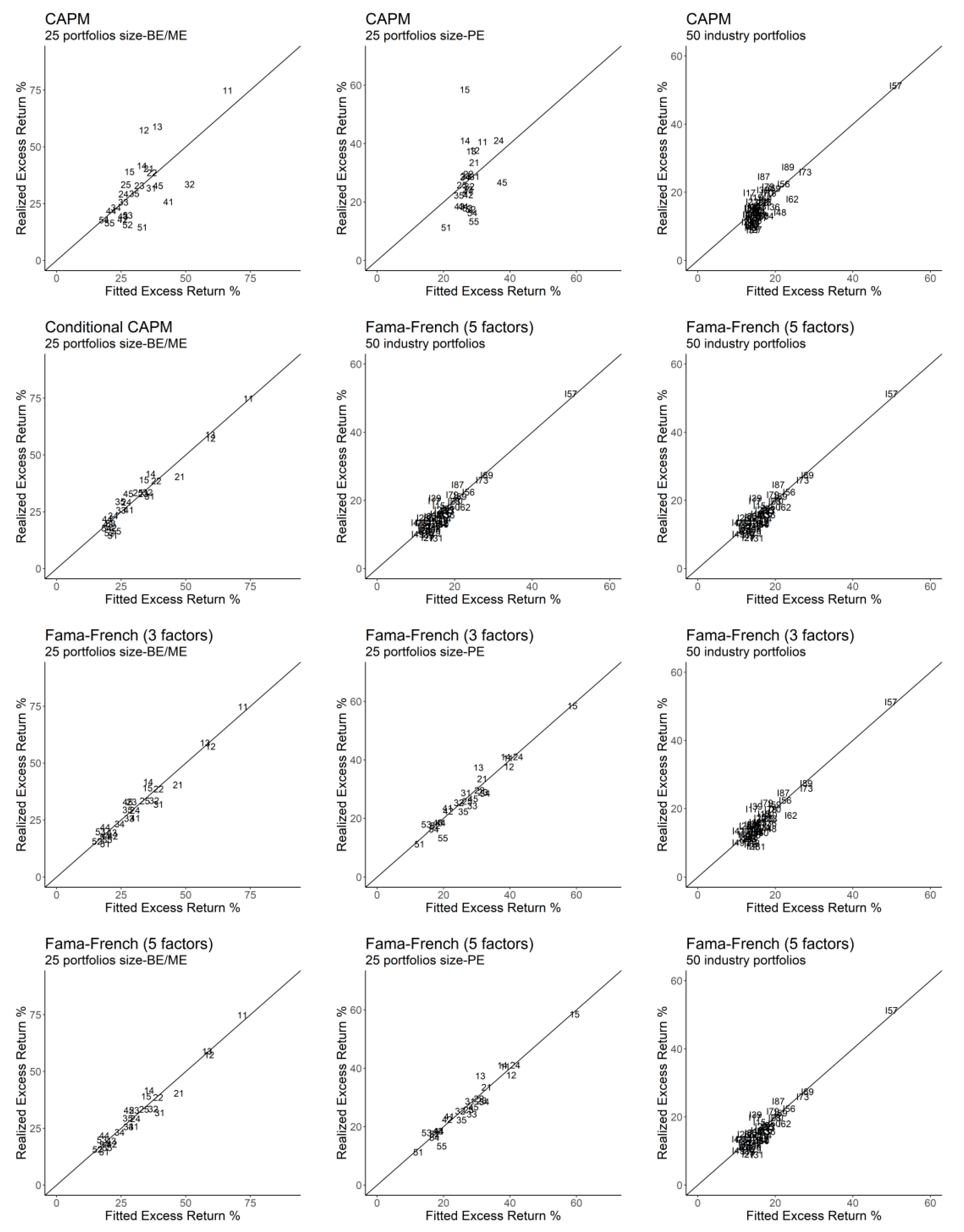
Figure 1 explicitly relates the fitted values provided by the models under analysis to the mean excess returns of our test assets in Table 2. Accordingly, the better the model performs, the more concentrated the estimates are around the 45 degree angle, and vice versa. In this regard, Figure 1 shows that the fitted values provided by the conditional CAPM satisfactorily track the average returns of most portfolios, resulting in patterns comparable to those of the Fama–French three- and five-factor models. On the other hand, the results provided by the unconditional CAPM are much more scattered, meaning that the model performs significantly worse, which is particularly evident for size-PE portfolios.

In summary, our results suggest that nuclear disasters help to largely explain the fraction of the expected returns that remains unexplained by the classic CAPM for the Japanese equity market. In this regard, our results show that the unconditional CAPM explains 49.6% of the cross-sectional variation of the expected returns of size-BE/ME portfolios, while the conditional CAPM captures 93.8% of such variation. Furthermore, in the case of size-PE portfolios, the unconditional and conditional CAPM provide OLS $R^2$ statistics of 0.102 and 0.907, respectively, suggesting that nuclear disasters are highly explanatory for these portfolios. Our results also show that most expected returns are positively related to nuclear disasters. However, as shown in Table 5, industry portfolios constitute an exception to this rule, which is a direct consequence of the small price of disaster risk ${\lambda }_z$ for these portfolios.

Importantly, the results shown in Table 3, Table 4 and Table 5 for the conditional CAPM indicate that, while the beta coefficients for zRMRF are statistically significant for most of the portfolios under study, the prices of risk for z and zRMRF are insignificant. These results suggest that nuclear disasters entail significant changes in the quantity of market risk of the stocks traded on the Japanese equity market, but have a much more limited effect on the prices of risk. Nevertheless, the results shown in Table 5 and Table A1 for the conditional CAPM indicate that nuclear disasters give rise to transitory effects on the risk premiums for size-BE/ME and size-PE portfolios. Specifically, while the estimates for ${\lambda }_{zRMRF}$ in Table 5 are positive and statistically insignificant on an annual basis, they turn out to be negative and statistically significant on a quarterly basis (see Table A1). This pattern is consistent with the results provided by other predictive variables, such as the consumption–wealth ratio, that help to forecast dividend growth or involve changes in the term structure of expected returns [24].

Finally, in order to determine the estimated variation in the cost of equity that would occur in the case of the mitigation of nuclear disasters, we analyze the difference between the fitted values provided by the conditional CAPM, as defined in expression (12), and the fitted values provided by the conditional CAPM in the absence of nuclear catastrophes. For that purpose, we assume that nuclear disasters do not affect the price of risk ${\lambda }_{R^w}$ or risk loadings ${\mathsf{\beta }}_{R^w}$, which means that the conditional CAPM in the absence of nuclear disasters is fully equivalent to expression (12), ignoring the second and third terms on the right-hand side. Thus, denoting the estimated conditional CAPM as “Model A” and the estimated conditional CAPM in the absence of nuclear disasters as “Model B”:

$$\mathrm{Model} \mathrm{A}: \tilde{E}\left(R_{t+\mathbf{1}}^e\right)={\tilde{\mathsf{\beta }}}_{RMRF}{\tilde{\lambda }}_{RMRF}+{\tilde{\mathsf{\beta }}}_z{\tilde{\lambda }}_z+{\tilde{\mathsf{\beta }}}_{zRMRF}{\tilde{\lambda }}_{zRMRF}$$

(14)

$$\mathrm{Model} \mathrm{B}: \tilde{E}\left(R_{t+\mathbf{1}}^e\right)={\tilde{\mathsf{\beta }}}_{RMRF}{\tilde{\lambda }}_{RMRF}$$

(15)

where the circumflex denotes estimated values. The betas in expressions (14) and (15) are taken from Table 3, while the lambdas are taken from Table 5. Therefore, the theoretical reduction in the cost of equity that would result from the complete elimination of nuclear disasters is given by the difference between expressions (14) and (15).

Table 6. Reduction in the cost of equity in the event of elimination of nuclear disasters.

Portfolio	Model A	Model B	Diff	Portfolio	Model A	Model B	Diff	Portfolio	Model A	Model B	Diff	Portfolio	Model A	Model B	Diff.
Panel A: 25 portfolios size-BE/ME				Panel B: 25 portfolios size-PE				Panel C: 50 industry portfolios
11	72.23	70.35	1.88	11	36.54	35.65	0.89	I13	12.88	15.25	−2.37	I41	10.81	12.89	−2.08
12	57.58	24.84	32.74	12	43.56	39.72	3.85	I14	14.08	17.91	−3.83	I42	13.8	14.62	−0.81
13	57.48	51.75	5.72	13	32.33	32.67	−0.34	I15	14.07	16.97	−2.9	I44	16.08	19.56	−3.48
14	34.41	33.11	1.3	14	32.78	32.87	−0.1	I16	12.44	14.49	−2.05	I45	11.49	13.51	−2.02
15	31.81	24.33	7.48	15	56.43	23.32	33.11	I17	10.95	13.03	−2.09	I47	14.72	16.19	−1.47
21	45.66	44.72	0.94	21	31.91	31.23	0.68	I20	10.23	11.57	−1.34	I48	18.35	16.12	2.23
22	36.58	37.45	−0.87	22	28.52	27.72	0.81	I22	12.88	15.84	−2.95	I49	10.89	11.94	−1.05
23	31.51	23.46	8.05	23	30.26	28.14	2.12	I23	12.13	14.31	−2.18	I50	16.29	17.76	−1.48
24	25.02	23.64	1.38	24	38.25	38.91	−0.66	I24	9.87	11.5	−1.63	I51	15.97	17.45	−1.48
25	29.5	26.62	2.88	25	25.53	23.95	1.58	I25	12.36	14.23	−1.87	I53	15.22	17.88	−2.66
31	33.97	35.29	−1.32	31	26.57	25.66	0.91	I26	10.98	12.35	−1.37	I54	14.84	13.85	0.99
32	33.26	36.72	−3.46	32	20.79	21.47	−0.68	I27	12.75	14.21	−1.46	I56	19.67	17.53	2.14
33	22.92	21.03	1.89	33	29.54	28.85	0.69	I28	11.11	12.45	−1.34	I57	48.16	32.75	15.41
34	19.87	18.8	1.07	34	26.54	22.71	3.84	I29	11.69	13.66	−1.98	I58	11.5	11.74	−0.24
35	22.6	21.09	1.51	35	23.67	23.47	0.2	I30	11.75	14.22	−2.47	I59	17.41	16.73	0.68
41	25.97	25.88	0.1	41	21.09	20.68	0.41	I31	12.42	14.74	−2.32	I60	15.91	18.14	−2.23
42	19.34	19.23	0.11	42	20.41	20.3	0.11	I32	12.22	14.64	−2.41	I61	13.6	14.95	−1.35
43	17.94	18.51	−0.57	43	15.57	15.22	0.35	I33	17.65	21.81	−4.16	I62	24.14	23.73	0.42
44	17.61	16.79	0.82	44	15.4	15.17	0.23	I34	12.43	15.25	−2.82	I63	12.84	15.01	−2.16
45	25.75	25.22	0.53	45	25.77	27.36	−1.58	I35	16.5	18.12	−1.63	I70	18.59	21.9	−3.31
51	19.7	20.3	−0.6	51	10.21	9.54	0.67	I36	17.7	17.28	0.42	I73	25.71	21.74	3.96
52	18.42	16.83	1.58	52	19.22	17.67	1.54	I37	13.49	14.86	−1.37	I78	17.13	17.7	−0.57
53	18.91	17.32	1.58	53	15.34	13.72	1.62	I38	13.02	13.25	−0.24	I79	16.67	17.51	−0.83
54	17.33	15.69	1.64	54	16.16	16.44	−0.27	I39	14.16	13.98	0.18	I87	18.89	23.59	−4.69
55	21.06	17.1	3.96	55	18.64	19.5	−0.86	I40	11.73	13.51	−1.78	I89	24.07	25.45	−1.39
	Average:		2.81		Average:		1.96						Average:		−1.11

Note: The columns labeled “Model A” show the fitted values provided by the conditional CAPM as determined using expression (14), while the columns labeled “Model B” show the fitted values provided by the conditional CAPM assuming a zero probability of nuclear disaster, as determined by expression (15). The table also shows the difference between these two series. All results are annual percentages.

shows the results provided by Models A and B for all the portfolios under consideration. Although the variation in the cost of equity for each portfolio differs depending on the risk loadings ${\tilde{\mathsf{\beta }}}_z$ and ${\tilde{\mathsf{\beta }}}_{zRMRF}$ in expression (14), Table 6 shows that the average reduction in the cost of equity for size-BE/ME portfolios in the case of a zero probability of a nuclear disaster amounts to 2.81%, while it is 1.96% for size-PE portfolios. Consistent with the results shown in Table 3 and Table 5, nuclear disaster mitigation does not imply a reduction but an increase of 1.11% in the discount rates of industry portfolios. Furthermore, the average reduction in the cost of equity for all the portfolios under analysis amounts to 1.22%.

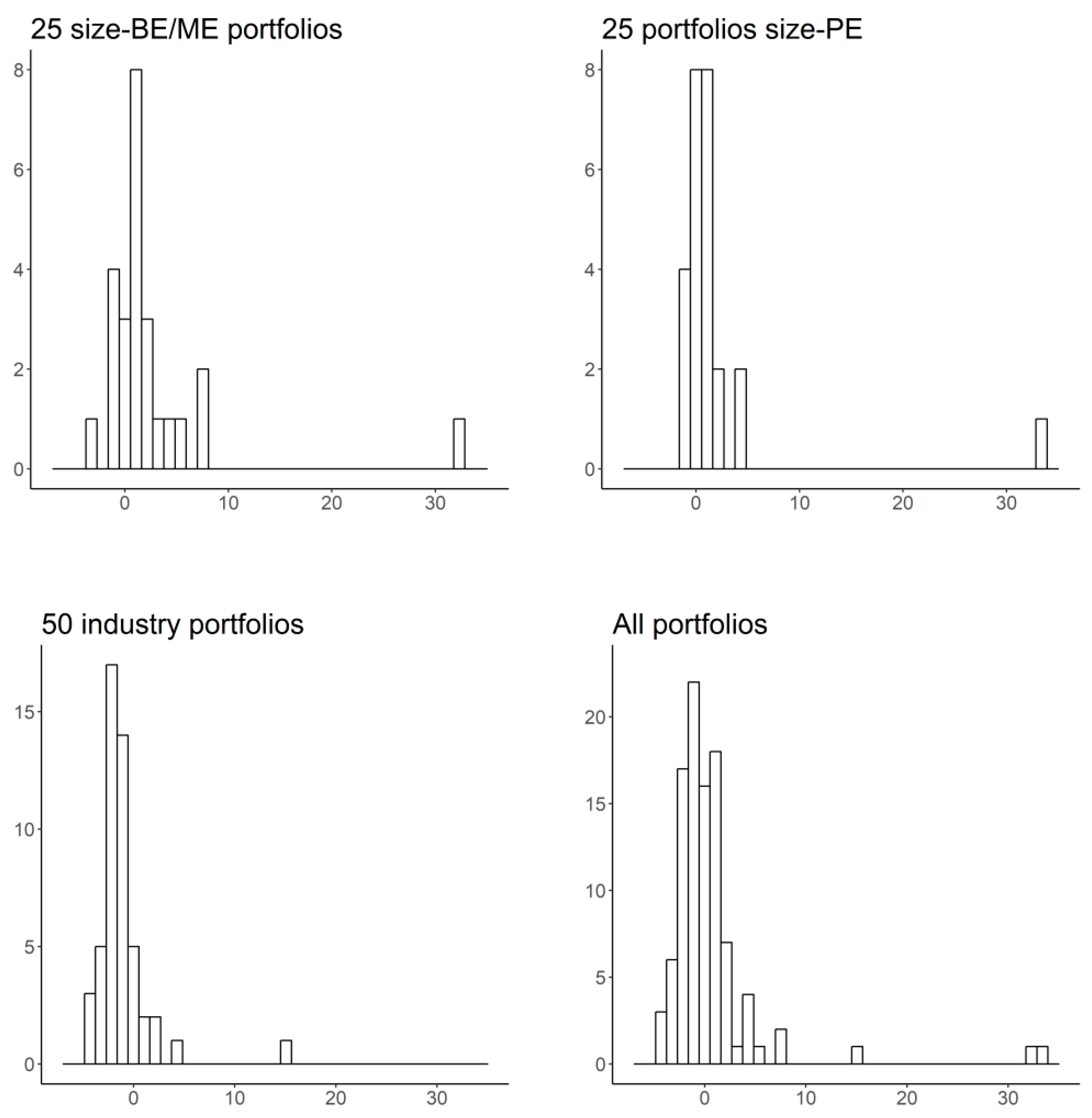
Nevertheless, it should be noted that the variations shown in Table 4 are highly volatile, yielding a standard deviation of 13.46%. Obviously, this means that the intensity of the effects of nuclear disaster mitigation on discount rates is highly dependent on the betas shown in Table 3. In this regard, it is important to highlight that the variation in the cost of equity follows a highly asymmetric distribution in all the portfolio sets. Furthermore, Figure 2 shows the histograms of the variations in Table 6 for the cost of equity, revealing that the average reduction in discount rates displays a markedly right-skewed pattern. This fact emphasizes the propensity of the cost of equity to decrease in the event of nuclear disaster mitigation, so the lower the number of nuclear disasters, the lower the cost of equity, and vice versa. As noted above, corporate value is highly dependent on discount rates, consistent with the mechanics of discounted cash flow models. In this regard, our results suggest that nuclear disaster mitigation can enhance value creation in the economy, contributing to significantly reducing the cost of capital in a large number of companies.

5. Conclusions

Recent experience has clearly underlined the catastrophic consequences of nuclear disasters in a wide variety of areas, ranging from geopolitics to public healthcare. From an economic point of view, the effects of nuclear disasters have traditionally been addressed from the perspective of energy supply and infrastructures, largely ignoring their important effects on financial markets and economic growth. In this framework, the increase in the cost of capital and the fall in consumer spending in the event of a nuclear disaster are major consequences of nuclear hazard that have not been sufficiently addressed in the literature. In particular, disincentives to invest stemming from the high perceived risk can largely become a barrier to social and economic development. Moreover, increased efforts to develop environmentally friendly energy not only can lead to a better protection of the environment, but also promote value creation and economic growth via lower costs of capital.

Building on the fact that discount rates are one of the key elements that drive investment decisions, this paper analyzed the effect of nuclear disasters on the performance of the CAPM, as it is by far the most widely used model in practice for determining the cost of equity. In particular, we studied the effect of nuclear catastrophes on investors’ perceptions using the CAPM and the role of conditioning information in the decisions of economic agents.

Our results show that nuclear disasters are positively related to the returns provided by a large fraction of the portfolios that constitute our test assets. Furthermore, our results show that the use of information on past nuclear disasters as part of the information sets used by investors to drive their economic decisions significantly helps the CAPM to improve its performance in explaining expected returns. Moreover, our approach allows the model to isolate the fraction of the cost of equity that results from the occurrence of nuclear disasters and, therefore, estimate discount rates in a context of the absence of nuclear disasters. Our results suggest that nuclear disasters and the cost of equity are positively related for most of the portfolios considered, although their exact relationships largely depend on the risk loadings shown in Table 3. In any case, the estimated variation in the cost of equity when we assume the absence of nuclear disasters is strongly right-skewed, which emphasizes the propensity of the cost of equity to decrease in the case of nuclear disaster mitigation.

Nevertheless, it should be noted that the above results are subject to the limitations imposed by the specific nature of nuclear disasters and, specifically, the fact that nuclear disasters occur rarely. This constraint reduces the number of years that comprise nuclear catastrophes in our sample to five out of a total of 35. Furthermore, while the return series of the portfolios under study comprise more than 3,000 stocks in the last years of the period considered, the missing accounting data at the beginning of the sample drastically reduce that number, which can lead to some measurement errors in betas.

Given the aforementioned findings, future research should address different aspects that naturally follow from our results. First, further research should study the extent to which these results persist in other countries with less exposure to nuclear hazard than Japan. Moreover, our methodology can easily be accommodated to the study of the spreads in the cost of equity that arise as a function of the orientation of economies towards clean energy and environmental policies. Second, our results suggest that the effect of nuclear disasters on the prices of risk is sensitive to the periodicity of data, which generates transitory effects on risk premiums. Future research should explore the predictive power of nuclear disasters at different horizons in order to determine the persistence of their effects over time. For that purpose, the Campbell–Shiller approximation for asset returns [61], as used by [24] for the dividend yield and the consumption–wealth ratio, could be an extremely useful tool. Furthermore, our model could greatly benefit from research on regimes followed by the economic consequences of nuclear disasters (e.g., consumption growth, gross domestic product, etc.), allowing the instrument $z_t$ to better capture the specific patterns followed by economic indicators across countries. Finally, further research on the firm-specific characteristics that determine the exposure of discount rates to nuclear disasters is essential.

References

- Sharif, A.; Dogan, E.; Aman, A.; Khan, H.H.A.; Zaighum, I. Rare disaster and renewable energy in the USA: New insights from wavelet coherence and rolling-window analysis. Nat. Hazards 2020, 2731–2755. [Google Scholar] [CrossRef]
- Yang, L.; Qin, H.; Gan, Q.; Su, J. Internal control quality, enterprise environmental protection investment and finance performance: An empirical study of China’s a-share heavy pollution industry. Int. J. Environ. Res. Public Health 2020, 17, 6082. [Google Scholar] [CrossRef] [PubMed]
- Gupta, R.; Suleman, T.; Wohar, M.E. The role of time-varying rare disaster risks in predicting bond returns and volatility. Rev. Financial Econ. 2018, 37, 327–340. [Google Scholar] [CrossRef]
- Sato, A.; Lyamzina, Y. Diversity of concerns in recovery after a nuclear accident: A perspective from Fukushima. Int. J. Environ. Res. Public Health 2018, 15, 350. [Google Scholar] [CrossRef] [Green Version]
- Kunsch, P.L.; Friesewinkel, J. Nuclear energy policy in Belgium after Fukushima. Energy Policy 2014, 66, 462–474. [Google Scholar] [CrossRef]
- Barro, R.J. Rare disasters and asset markets in the twentieth century. Q. J. Econ. 2006, 121, 823–866. [Google Scholar] [CrossRef]
- Barro, R.J. Rare disasters, asset prices, and welfare costs. Am. Econ. Rev. 2009, 99, 243–264. [Google Scholar] [CrossRef] [Green Version]
- Gabaix, X. Variable rare disasters: An exactly solved framework for ten puzzles in macro-finance. Q. J. Econ. 2012, 127, 645–700. [Google Scholar] [CrossRef] [Green Version]
- Rietz, T.A. The equity risk premium a solution. J. Monetary Econ. 1988, 22, 117–131. [Google Scholar] [CrossRef]
- Sharpe, W.F. Capital asset prices: A theory of market equilibrium under conditions of risk. J. Financ. 1964, 19, 425–442. [Google Scholar] [CrossRef] [Green Version]
- Lintner, J. The valuation of risk assets and the selection of risky investments in stock portfolios and capital budgets. Rev. Econ. Stat. 1965, 47, 13. [Google Scholar] [CrossRef]
- Lintner, J. Security prices, risk, and maximal gains from diversification. J. Financ. 1965, 20, 587–615. [Google Scholar]
- Cochrane, J.H. A cross-sectional test of an investment-based asset pricing model. J. Political Econ. 1996, 104, 572–621. [Google Scholar] [CrossRef]
- Ferson, W.E.; Schadt, R.W. Measuring Fund Strategy and Performance in Changing Economic Conditions. J. Financ. 1996, 51, 425–461. [Google Scholar] [CrossRef]
- Cochrane, J.H. Asset Pricing, Revised Edition; Princeton University Press: Princeton, NJ, USA, 2005. [Google Scholar]
- Yogo, M. A consumption-based explanation of expected stock returns. J. Financ. 2006, 61, 539–580. [Google Scholar] [CrossRef] [Green Version]
- Jagannathan, R.; Wang, Y. Lazy investors, discretionary consumption, and the cross-section of stock returns. J. Financ. 2007, 62, 1623–1661. [Google Scholar] [CrossRef] [Green Version]
- Lutzenberger, F. Multifactor models and their consistency with the ICAPM: Evidence from the European stock market. Eur. Financ. Manag. 2014, 21, 1014–1052. [Google Scholar] [CrossRef]
- Campbell, J.Y.; Giglio, S.; Polk, C.; Turley, R. An intertemporal CAPM with stochastic volatility. J. Financ. Econ. 2018, 128, 207–233. [Google Scholar] [CrossRef] [Green Version]
- Lettau, M.; Ludvigson, S. Resurrecting the (C) CAPM: A cross-sectional test when risk premia are time-varying. J. Political Econ. 2001, 109, 1238–1287. [Google Scholar] [CrossRef] [Green Version]
- Lustig, H.N.; Van Nieuwerburgh, S.G. Housing collateral, consumption insurance, and risk premia: An empirical perspective. J. Financ. 2005, 60, 1167–1219. [Google Scholar] [CrossRef]
- Merton, R.C. An Intertemporal Capital Asset Pricing Model. Econometrica 1973, 41, 867. [Google Scholar] [CrossRef]
- Campbell, J.Y. Consumption-Based Asset Pricing. SSRN Electron. J. 2002. [Google Scholar] [CrossRef] [Green Version]
- Cochrane, J.H. Presidential address: Discount rates. J. Financ. 2011, 66, 1047–1108. [Google Scholar] [CrossRef] [Green Version]
- Banz, R.W. The relationship between return and market value of common stocks. J. Financ. Econ. 1981, 9, 3–18. [Google Scholar] [CrossRef] [Green Version]
- Basu, S. The relationship between earnings’ yield, market value and return for NYSE common stocks. J. Financ. Econ. 1983, 12, 129–156. [Google Scholar] [CrossRef]
- Rosenberg, B.; Reid, K.; Lanstein, R. Persuasive evidence of market inefficiency. J. Portf. Manag. 1985, 11, 9–16. [Google Scholar] [CrossRef]
- Jegadeesh, N.; Titman, S. Returns to buying winners and selling losers: Implications for stock market efficiency. J. Financ. 1993, 48, 65–91. [Google Scholar] [CrossRef]
- Ang, A.; Hodrick, R.J.; Xing, Y.; Zhang, X. The cross-section of volatility and expected returns. J. Financ. 2006, 61, 259–299. [Google Scholar] [CrossRef] [Green Version]
- Cooper, M.J.; Gulen, H.; Schill, M.J. Asset growth and the cross-section of stock returns. J. Financ. 2008, 63, 1609–1651. [Google Scholar] [CrossRef]
- Fama, E.F.; French, K.R. Dissecting anomalies. J. Financ. 2008, 63, 1653–1678. [Google Scholar] [CrossRef]
- Novy-Marx, R. The other side of value: The gross profitability premium. J. Financ. Econ. 2013, 108, 1–28. [Google Scholar] [CrossRef] [Green Version]
- Van Binsbergen, J.H.; Opp, C.C. Real Anomalies. J. Financ. 2019, 74, 1659–1706. [Google Scholar] [CrossRef]
- Leland, H.E. Insider trading: Should it be prohibited? J. Political Econ. 1992, 100, 859–887. [Google Scholar] [CrossRef]
- Subrahmanyamand, A.; Titman, S. Feedback from Stock Prices to Cash Flows. J. Financ. 2001, 56, 2389–2413. [Google Scholar] [CrossRef]
- Goldstein, I.; Ozdenoren, E.; Yuan, K. Trading frenzies and their impact on real investment. J. Financ. Econ. 2013, 109, 566–582. [Google Scholar] [CrossRef]
- Hansen, L.P.; Richard, S.F. The role of conditioning information in deducing testable restrictions implied by dynamic asset pricing models. Econometrica 1987, 55, 587. [Google Scholar] [CrossRef] [Green Version]
- Ross, S.A. The arbitrage theory of capital asset pricing. J. Econ. Theory 1976, 13, 341–360. [Google Scholar] [CrossRef]
- Roll, R.; Ross, S.A. An empirical investigation of the arbitrage pricing theory. J. Financ. 1980, 35, 1073–1103. [Google Scholar] [CrossRef]
- Fama, E.F.; French, K.R. Common risk factors in the returns on stocks and bonds. J. Financ. Econ. 1993, 33, 3–56. [Google Scholar] [CrossRef]
- Carhart, M.M. On persistence in mutual fund performance. J. Financ. 1997, 52, 57–82. [Google Scholar] [CrossRef]
- Fama, E.F.; French, K.R. A five-factor asset pricing model. J. Financ. Econ. 2015, 116, 1–22. [Google Scholar] [CrossRef] [Green Version]
- Rojo-Suárez, J.; Alonso-Conde, A.B.; Ferrero-Pozo, R. European equity markets: Who is the truly representative investor? Q. Rev. Econ. Financ. 2020, 75, 325–346. [Google Scholar] [CrossRef]
- Cochrane, J.H. Financial markets and the real economy. In Handbook of the Equity Risk Premium; Elsevier: Amsterdam, The Netherlands, 2008; pp. 237–325. [Google Scholar]
- Weitzman, M.L. Subjective expectations and asset-return puzzles. Am. Econ. Rev. 2007, 97, 1102–1130. [Google Scholar] [CrossRef] [Green Version]
- Martin, I.W.R. Consumption-based asset pricing with higher cumulants. Rev. Econ. Stud. 2012, 80, 745–773. [Google Scholar] [CrossRef]
- Pindyck, R.S.; Wang, N. The economic and policy consequences of catastrophes. Am. Econ. J. Econ. Policy 2013, 5, 306–339. [Google Scholar] [CrossRef] [Green Version]
- Wachter, J.A. Can time-varying risk of rare disasters explain aggregate stock market volatility? J. Financ. 2013, 68, 987–1035. [Google Scholar] [CrossRef] [Green Version]
- Liu, B.; Niu, Y.; Yang, J.; Zou, Z. Time-varying risk of rare disasters, investment, and asset pricing. Financ. Rev. 2020, 55, 503–524. [Google Scholar] [CrossRef]
- Wang, Y.; Mu, C. Can ambiguity about rare disasters explain equity premium puzzle? Econ. Lett. 2019, 183, 108555. [Google Scholar] [CrossRef]
- Ross, S.A. A simple approach to the valuation of risky streams. J. Bus. 1978, 51, 453. [Google Scholar] [CrossRef]
- Harrison, J.; Kreps, D.M. Martingales and arbitrage in multiperiod securities markets. J. Econ. Theory 1979, 20, 381–408. [Google Scholar] [CrossRef]
- Huang, J.-Z. The valuation of uncertain income streams and the pricing of options. In Handbook of Quantitative Finance and Risk Management; Springer: Berlin/Heidelberg, Germany, 2010; pp. 605–616. [Google Scholar]
- Fama, E.F.; French, K.R. International tests of a five-factor asset pricing model. J. Financ. Econ. 2017, 123, 441–463. [Google Scholar] [CrossRef]
- Griffin, J.M.; Kelly, P.J.; Nardari, F. Do market efficiency measures yield correct inferences? A comparison of developed and emerging markets. Rev. Financ. Stud. 2010, 23, 3225–3277. [Google Scholar] [CrossRef]
- Alonso-Conde, A.B.; Rojo-Suárez, J. Data for: Nuclear hazard and asset prices: Implications of nuclear disasters in the cross-sectional behavior of stock returns. Mendeley Data 2020. [Google Scholar] [CrossRef]
- Fama, E.F.; Macbeth, J.D. Risk, return, and equilibrium: Empirical tests. J. Political Econ. 1973, 81, 607–636. [Google Scholar] [CrossRef]
- Shanken, J. On the estimation of beta-pricing models. Rev. Financ. Stud. 1992, 5, 1–33. [Google Scholar] [CrossRef]
- Hansen, L.P. Large sample properties of generalized method of moments estimators. Econometrica 1982, 50, 1029. [Google Scholar] [CrossRef]
- Lewellen, J.; Nagel, S.; Shanken, J. A skeptical appraisal of asset pricing tests. J. Financ. Econ. 2010, 96, 175–194. [Google Scholar] [CrossRef] [Green Version]
- Campbell, J.Y.; Shiller, R.J. The dividend-price ratio and expectations of future dividends and discount factors. Rev. Financ. Stud. 1988, 1, 195–228. [Google Scholar] [CrossRef] [Green Version]
Figure 1.
Realized excess returns versus fitted values. We depict 25 portfolios size-BE/ME according to a code with two numbers, the first number being the size code (with 1 being the smallest and 5, the largest) and the second number being the BE/ME ratio code (with 1 representing a low ratio and 5, a high ratio). Size-PE portfolios are also represented by a code with two numbers, the first number being the size code (as in size-BE/ME portfolios, 1 is the smallest size and 5, the largest size) and the second number being the PE ratio code (with 1 representing a low ratio and 5, a high ratio). We depict industry portfolios according to the letter “I” followed by the first two digits of the SIC code.
Figure 2.
Histograms for the reduction in the cost of equity in the event of elimination of nuclear disasters.