Human Impact Promotes Sustainable Corn Production in Hungary


1
Centre for Agricultural Research Institute of Hungary, H-2462 Martonvásár, Hungary
2
Department of Meteorology, Eötvös Loránd University, H-1117 Budapest, Hungary
3
Research Institute of Agricultural Economics, H-1093 Budapest, Hungary
4
Department of Geophysics and Space Science, Eötvös Loránd University, H-1117 Budapest, Hungary
*
Author to whom correspondence should be addressed.
Sustainability 2020, 12(17), 6784; https://doi.org/10.3390/su12176784
Submission received: 30 June 2020
/
Revised: 12 August 2020
/
Accepted: 13 August 2020
/
Published: 21 August 2020
(This article belongs to the Special Issue Sustainability of Farming in Future: Developing of Sustainable Intensification)
Abstract
:We aim to predict Hungarian corn yields for the period of 2020–2100. The purpose of the study was to mutually consider the environmental impact of climate change and the potential human impact indicators towards sustaining corn yield development in the future. Panel data regression methods were elaborated on historic observations (1970–2018) to impose statistical inferences with simulated weather events (2020–2100) and to consider developing human impact for sustainable intensification. The within-between random effect model was performed with three generic specifications to address time constant indicators as well. Our analysis on a gridded Hungarian database confirms that rising temperature and decreasing precipitation will negatively affect corn yields unless human impact dissolves the climate-induced challenges. We addressed the effect of elevated carbon dioxide (CO2) as an important factor of diverse human impact. By superposing the human impact on the projected future yields, we confirm that the negative prospects of climate change can be defeated.
1. Introduction
Empirical studies put various climate, biophysical, and economic models in practice for assessing the impact of climate change on crop yields. The results and inferences vary due to model singularities, differences in input data, and the heterogeneity of global food production areas [1,2,3,4,5]. Applications on a global scale have the potential to predict average global yields (under reported uncertainty) for the most important commodities with rather simple measures of highly aggregated growing season temperature and precipitation [6,7,8]. Nevertheless, there are many locally changing factors that likely affect corn yields—including political stability, land use, soil organic matter content, as well as the implementation of technological and agronomic developments—which researchers are unable to properly quantify and are thus cumbersome for modeling purposes. Drawing global supply and demand trends and understanding future challenges of food security are vitally important, but shaping targeted agricultural policy making requires more detailed information about the internal functioning of agents. Therefore, we argue to conceive studies with smaller spatial coverage, where essential local drivers may be considered and agronomic weather measures are executed at the potentially smallest (but realistic) gridded resolution to capture the most spatial heterogeneity and greatest data variability to decrease uncertainties.
1.1. On Hungarian Corn Production
Corn production is one of the most valuable sectors of Hungarian agriculture. Hungary has the fourth-largest production area of corn in the European Union (EU), which takes up about 1–1.3 million hectares depending on the state of crop rotation [9]. Due to climatic, industrial, and demographic reasons, there is an increasing demand for corn in Europe [10,11,12]. Among the European Member States, Hungary serves the second-largest corn export (after France), with the mean capacity of 3.7 million tons a year (based on the average production of 2007–2015 [13]). Studies show that Hungary’s climate is on the verge of humid oceanic, dry continental, and Mediterranean climate regions that is responsible for the highly variable weather [14]. The climate within the Carpathian Basin has become warmer and drier in the agriculturally most important period of the year: from May to September [15,16]. Extreme weather events cause unequal rainfall distribution on Hungarian land and negatively influence soil fertility through natural water supply. Different soils react differently to the stress effects evolved as a result of lacking precipitation, so their drought sensitivity will not be the same [17]. There is a marked tendency that drought and heat stress have become more common, which had a strong negative impact on corn yields in several years [18,19].
Figure 1 shows the courses of Hungarian and European corn yields over the baseline period of 1970–2018. The volatility of Hungarian corn yield is higher than the European, although in this long time series, corn yields have nearly doubled for both graphs.
By explaining the relation of Hungarian and European corn yield charts, we underline the historic moment in 1990, when the Soviet Union collapsed and the satellite states like Hungary could start the process of democratic transformation. Under the Communist Regime, Hungarian farmers were forced to work in production cooperatives on confiscated land and destroyed the historically developed agricultural society of gentries. In lack of environmental considerations and climate protections, an unreasonably large amount of imported nonorganic fertilizer was used for mass cultivation. Large portions of the produced agricultural commodities were transported and absorbed by the Comecon markets. The planned socialist economy took a positive effect on Hungarian corn yields (i.e., it largely exceeded the European average yield), but it exploited farmland and caused serious environmental problems. The political transformation brought the termination of fertilization subsidies, the era of legal redresses, and compensations, which resulted in an enormous setback in agricultural yields compared to the rest of Europe in the beginning of the 1990s. Later, by the second half of the decade, the recouped agricultural society rehabilitated and reorganized agricultural production conditions and started to compete on new European markets. However, nothing illustrates better the current imperfections of Hungarian agricultural convergence, when the emergent occasions of adverse weather conditions affect less negatively the aggregated European corn yields, than the Hungarian corn production (see Figure 1, years of 2000, 2003, 2007, 2012). This implies that Hungary is more vulnerable to negative environmental impacts. Therefore, the financial stability is at stake of the export-driven corn production system in the light of climate change. In this manner, we reveal the fundamental challenge of future farming as to whether the development of adaptive capacity in Hungary will exceed the European improvement.
1.2. Motivation and Contribution
The aim of the study was to model the environmental and social impact indicators and explain the observed year-specific yield fluctuations. We analyzed the highly variable weather and other important production factors on historic corn yields (1970–2018) and used the responses to predict future yields for the period of 2020–2100. We intended to present the impact of climate change by employing various climate projections, but more importantly, we desired to reveal that persisting human impact may increase adaptive capacity and efficiently tackle the potential negative impact of climate change. We applied the within-between random effect model on our balanced panel dataset to account for other substantial factors such as agronomic improvements and individual characteristics beyond weather variabilities.
First, we compiled a new data set that integrates the spatial distribution of yields, soil characteristics, and a number of climatic variables for the total coverage of Hungary at a 10 km × 10 km grid resolution. Second, we delineated a time trend that we associate with the cumulated human impact towards improving corn yields. Third, we estimated simultaneously three model specifications with respect to diversified variable settings and decomposed growing season periods (i.e., distinguishing vegetative and reproductive growth phases).
The rest of the paper is divided into four parts. In Section 2, we argue the binding assumptions of individual homogeneity, introduce the rest of the data and present the applied method. In Section 3, we interpret the results and discuss the most important implications; Section 4 summarizes the conclusions.
2. Materials and Methods
2.1. Biophysical and Social Environment
Earlier, Hungarian agricultural commodity yields were assessed by process-based crop models [20,21]. These are designed to calculate crop yield (and other important parameters of the soil-plant system) as a function of weather and soil conditions, stipulate plant-specific characteristics, and take the basic crop management steps into account. Crop-model-based studies find corn yield critically sensitive to rising temperature on Hungarian rain-fed arable land [21,22]. Despite their advantages [23,24,25,26,27], crop models are limited in their ability to express the continuous development in agrotechnology (e.g., use of slow-release fertilizer, progress in hybrid research, and evolving methods in application of pesticide: the increasing quality of agricultural operations in general) [28] and agromanagement (e.g., organizing cooperatives for more efficient production, utilization of farm-to-fork strategies). We argue that the differences in model approaches are not superior to each other; on the contrary, they are rather complementary where the grounded research interest determines the applied modeling strategy. As our research objective is built on revealing the factors of corn yield development, we used a stochastic approach with panel data to make more sufficient projections with the inclusion of progressive human impact.
Generally, farmers’ adaptive capacity to any change, especially to weather variabilities, is highly heterogeneous, due to the differences in factor endowments, production capacity, education, and experience, etc.; thus, it is a source of uncertainty and potential bias trap in stochastic modeling. Lately, global scale empirical models have been gaining ground in the scientific literature [29,30,31], but they are restrained to simulate yield responses when cropping areas shift [6,30] or easily lead to heterogeneity bias as the within-country differences are overlooked. Therefore, we suppose that the conclusions of global studies on future yield trends may be partially misleading, but in lack of a better global tool, it remains considerable.
We address the binding issue of individual homogeneity with small-scale grid resolution and link to the explicit assumption that agricultural producers aim to achieve the potentially highest yields in every year under given circumstances, regardless of occurring individual differences in production endowments and in adaptive capacity. Instead of neglecting all agromanagement, infrastructural, and policy considerations per se—due to identification challenges—we propose to control these unobserved variabilities based on preceding adjustments. Still, the real farm-level differences are disregarded by using gridded data, but spatial proximity within the grid cells is assumed to imply some similarity in unobserved human factors [32].
The underlined simplification on farmers’ behavior that they constantly maximize corn yields allows us to observe the aggregates of all unobserved effects in each year, which we perceive as the annual country aggregate of human impact towards increasing yields under variable weather and changing climate in the long run. In recent studies, technology improvements are taken for granted in the future, and models typically account for new technology by including some exogenous rate of growth in yields [33,34,35,36]. We argue that identifying the effect of a specific technological innovation is extremely difficult due to time lags and data shortage. We question the exclusive role of technology in the observed positive yield shifts. We believe that, in reality, achieving crop yield growth is a complex work at different levels. At the farm level, it is a process of making sequential decisions at every stage of the production under contrasting environmental settings (i.e., weather variability) that may simply include intensification (e.g., use of higher NPK doses), or finding more suitable hybrids. At the regulatory level, it is a process of providing a sustainable and resilient policy framework that supports healthy competitiveness, presents affordable financial assets for farmers, and administers the undergoing proprietary rights issues (e.g., tenancy in common affairs). The broad spectrum of human impact extends to agrotechnological development (crop breeding, technical advances, increasing factor endowments), policy environment (subsidy policy, political establishment), agricultural R&D and its translation into practice, knowledge spillovers, and capital accumulation. We acknowledge that the driving force of human impact is sourced from technological and agromanagement improvements for upward-trending yields, but we are aware of nontechnical aspects such as cooperation and knowledge transfer that substantially contribute to increase farm efficiency. In statistical crop models, when they refer to technology in the equation either by using state-specific quadratic time trends or year-fixed effects, they actually address the aggregate human impact [6,36,37,38].
Furthermore, there is an increasing need to clarify the effect of elevated CO2 on corn production, especially when long-term projections are considered. According to Leakey et al. [39], CO2 does not directly stimulate C4 photosynthesis, but can indirectly stimulate carbon assimilation in times and places of drought. Weigel and Manderscheid [40] recorded practically zero yield increase in wet conditions but over 40% yield gain in dry conditions. We address elevated CO2 and give 20% yield growth of maze as an upper estimate in case of a 200 ppm CO2 increase (from 350 ppm to 550 ppm) based on long-term Free Air CO2 Enrichment (FACE) experiments and crop model simulations [41]. Combining this figure with the ca. 80 ppm CO2 level increase of the observation period (1970–2018), we forecast about 8 kg/ha/year corn yield increase due to elevated CO2. We argue that this effect has been absorbed into the human impact trend in the past, but the decomposition of elevated CO2 and the rest of human impact is feasible for the future.
2.2. Data
The accumulated dataset consists of 1104 (approx. 10 × 10 km) grid cells, which constitutes a balanced panel of 49 years over the period of 1970–2018. Average corn yields for each grid cell were obtained from the Research Institute of Agricultural Economics (RIAE) and from the Hungarian Central Statistical Office (HCSO). Yield averages for the period of 2011–2018 were collected from the Hungarian model farm network that includes about two thousand farms. RIAE has developed this form of data accumulation representatively by model farms covering arable land of Hungary. The spatial distribution of yields over the 1104 grid cells was determined by attributing the model farm yields to the spatial grid system, where the farm is located. The county (NUTS-3)-level HCSO yield data that is available for the period of 1970–2010 is correspondingly spatially disaggregated for the grid cells by using the spatial distribution patterns of the model farm network data. Thus, the continuous dataset incorporates the inconceivable effects of various political establishments, reflects the specific policy or management choices, as well as assimilates technological development which, in use, may more reliably predict future corn yield responses. We draw attention to the long time span of the baseline yield data, where advances in management practices, crop improvement, technical and nontechnical changes mutually affected agricultural productivity.
The observed meteorological and simulated future climate datasets were provided by the FORESEE database [42]. The FORESEE v3.1 [43] is derived from the E-OBS 17e dataset [44] for the historical time period (1951‒2018), and from the ENSEMBLES project [45] for the future projections based on the SRES A1B emission scenario [46]. Though, the production of RCP (Representative Concentration Pathways)-based climate projections has been started, at present, FORESEE v3.1 is the only database meeting all the criteria required for this study: (1) observed data covers the study area with the required spatial resolution; (2) observed data covers the investigated time period; (3) climate projections (future data) have the same spatial resolution than that of the observed data and contain continuous daily data up to 2100; (4) climate projections are bias-corrected using the observed data of the database from a reference period that includes the investigated period; (5) the incorporated regional climate and global climate models (RCM-GCM) cover a sufficiently wide range, as for temperature and especially for precipitation, the RCM-GCM selection-related uncertainty is usually larger than the scenario-selection-related uncertainty [47]. The FORESEE v3.1 database provides spatially interpolated meteorological fields for Central Europe for the period of 1951–2100. The bias-corrected, projected time series were derived by using 10 different RCMs embedded in three different GCMs [42]. The data at the original FORESEE resolution of 1/6° × 1/6° was resampled to the finer resolution of 0.1° × 0.1°, in accordance with the gridded corn yield data of the 1104 cells. Kern et al. [48] developed the applied methodology for the spatial transformation, with respect to elevation attributes.
In this paper, we selected six climate projections to present uncertainty for the period of 2020‒2100 and assess the climatic response of Hungarian corn yield for different scenarios. As temperature and precipitation are the most influential indicators for corn development, we opted for showing the positive and negative extremes as well as the average projections for both impact indicators. By selecting the RCMs, we considered separately the mean temperature and the precipitation sums in the growing season for the period of 2071‒2100. Table S1 shows the decadal mean and standard deviation of the respective climatic measures. The FORESEE v3.1 is structured by daily minimum/maximum temperatures and precipitation sums. We supplemented the basic dataset by deriving daylight average temperature and shortwave radiation flux (i.e., global radiation) on the same grid by using the widely validated MTClim model [49].
The gridded weather data products use spatial interpolation to incorporate the accessible time-variant weather station data into the panel structure of observations on a fixed spatial scale of 1104 grid cells. To account for the impact of temperature, we used the well-established nonlinear formulation of degree days, also known as Growing Degree Days (GDD) [50,51,52]. GDD (Thermal Time) is a measure of heat accumulation calculated by taking the integral of warmth above a base temperature. As daily data is used in the study thermal, time is approximated with , where and are the daily maximum and minimum temperature and is the base temperature which is set to 8 °C. GDD is the sum of daily values for the given period. For identifying heat stress, we aggregated the Number of Hot Days (NHD), when the daily maximum temperature exceeds 30 °C for the given period. In addition, for further specifications, we obtained the total short-wave Radiation (RAD), measured in MJ/m2, considered wavelength between 0.2 μm and 3.0 μm from the sky falling onto a horizontal surface on the ground for the given period. Lastly, the simple measure of precipitation sum (P) was used for the given period measured in cm (Figure S1).
For the straightforward extension of the estimation methodology, we address the important subset of grid-cell-specific time-invariant measures of soil conditions. The soil data was retrieved from the 10 km resolution Digital, Optimized, Soil Related Maps and Information (DOSoReMI) database [53]. DOSoReMI is an observation-based dataset where locally measured soil parameters—Soil Organic Matter content (SOM), sand fraction, and pH—are spatially interpolated with the help of geophysical, terrain, land cover, and remotely sensed data. The native resolution of DOSoReMI is 100 m, but versions with coarser resolution are available up to a 10 km resolution. SOM and sand fraction are measured in percentage points of the topsoil (0–30 cm).
We explored the various interactions of the specified variables, although theoretically some may have an inverted U-shape for corn yield. Therefore, in our model specification, we define the squared terms of GDD, RAD, and P to account for potential higher-order interactions as well. As a null hypothesis, we expected GDD, P, RAD, SOM, and pH to positively correlate with corn yield and, on the contrary, the NHD, sand fraction, GDD2, RAD2, and P2 to negatively affect corn yields. The spatial distribution of yield and the most important weather measures are illustrated in Figure S1. The vegetation period (VP) cell values are aggregated for the period of 2009–2018.
2.3. Methodology
Fixed-effects (FE) modeling is used more frequently in applied econometric analysis, reflecting its status as the “gold standard” [54]. However, random-effects (RE) models have gained increasing prominence in various scientific fields [55,56,57] due to their greater flexibility and generalizability. Both methods are applicable to address complex research questions, including nested neighborhood relations [58,59,60] and temporal hierarchies [57,61].
Many research problems in agricultural economics, especially related to future production issues in light of climate change, describe the quantitative matter with hierarchical data structure. It is imposed during data collection as there are repeated measures over time at Level 1 (i.e., highly variable occasions, e.g., weather events) and nested in individuals at Level 2 (‘higher-level entities,’ e.g., countries, grid cells, etc.), which may include time-independent characteristics [61,62,63]. There are a large number of different model specifications in terms of choosing the appropriate model framework, functional form, and including the most meaningful/influential covariates. Still, FE models are regularly employed to avoid the problem of individual heterogeneity bias and control out all between effects by including the higher-level entities as dummy variables, e.g., [38]; however, the great advantage of FE models comes at a price of being unable to estimate the effects of higher-level processes and only dealing with occasion-level processes [61]. Therefore, FE models may not be practical in applications where time-invariant covariates (i.e., has only higher-level variance) are of particular interest, as they lose a large amount of information.
Mundlak [64,65] worked out his solution to this issue by adding the higher-level mean of each time-varying covariate in the model (the so-called Mundlak device) to explicitly account for the between effect instead of controlling it out. The Mundlak device is treated in the same way as any higher-level variable (i.e., time-invariant variable) and performs the covariates within a simple parsimonious RE framework. This yields to the same results as a FE model, but supplemented with the between effects in addition to other time-invariant variables of interest [62].
We used the most general parametrization of the Mundlak model, which is able to model both within- and between-individual effects concurrently, and also explicitly models heterogeneity in the effect of predictor variables at the individual level [63]:
This model is also called the ‘within-between RE’ model, where is the dependent variable, is a set of time-varying independent variables, and is a set of time-invariant independent variables. Each variable of is divided into two parts, and , representing the average within and between effects, respectively. The parameter exclusively stands for the between effect of the specific variable, as it has no within effect due to the lack of variation in time. The random setting of the model includes two terms: a random effect that is attached to the intercept () and another random term attached to the within slope (). Each of these is assumed to be normally distributed. Finally, is a grid-specific parameter on annual linear time trend to identify annual shocks and long-time improvements.
The scope of the paper is to determine the effect of highly variable occasions, such as biophysical effects of heat units, wetness/humidity, and nested grid object information of soil organic matter, pH, and sand consistency on observed corn yields. Our model specification closely follows the innovations published by Roberts et al. [38] and Auffhammer et al. [30], but applying the within-between random effects model stated above. Three generic model specifications were performed subject to the involved variables. Each model has two sub-specifications (i.e., ‘Model A’ and ‘Model B’) conditional on assuming a coupled or decoupled growing season (i.e., distinguishing plant development phases to vegetative and reproductive growth periods). Specification “A” includes the variables in coupled form, corresponding to mainstream variable use; while specification “B” incorporates GDD, RAD, and P in decoupled forms. The included variable structures are listed in Table 1.
Furthermore, we made predictions for corn yield of each of the regression models replacing observed weather data with projected future weather. Instead of removing trending human impact from the model (i.e., detrending the raw data), and thus exclusively accounting for the climate-change-induced differences in yield [38], we rather superposed the predicted human impact when making predictions for the future. Additionally, we relied on the works of Weigel and Manderscheid [40] and Castano-Sanches [41] with respect to the effect of elevated CO2 on corn yield, and disjointed this absorbed effect from the human impact. Methodologically, it means an artificial 8 kg/ha/year shift of the dependent variable. Though we know that the actual trend is highly dependent on the greenhouse gas concentration trajectory, this rate of elevated CO2-induced yield rise is assumed to be continuous in future decades, regardless of other aspects of human impact. Hereby, we were able to make predictions for future corn yield conformation either by assuming persistent human impact with absorbed CO2, or no human impact but elevated CO2 effect. Later at yield predictions, we designated the results with and without persisting human impact.
The applied REWB models can be fit in modeling software packages such as R, Stata, or SPSS. They are considered random-effects models with the mean of included as an additional explanatory variable [66]. We used “plm,” ”lme4,” and “Metrics” packages in R for calculation [67,68,69] and “plotly” for visualization [70].
3. Results
We parametrize six models, all of which are presented in Table 2. The ‘A’ and ‘B’ specifications indicate whether we consider the growing period in its overall length or differentiate the major plant growth phases.
In all model specifications, we found the 49-year linear time trend significant and positive on Hungarian corn yields. Yet, we mutually accounted for all types of human impacts, including elevated CO2. With all models, we calculated between 77 and 81 kg/ha of average yield increase. The results of temperature indicators confirm our initial hypothesis that increasing GDD and RAD will contribute to corn yield growth, although under “B” specifications, we reveal some negative and significant estimates. This suggests that increasing temperature in the vegetative plant development phase may set back the potential yield. Correspondingly, the within effect of heat stress (NHD) caused decreasing yields in all cases. (The within and between effects have different substantive meanings as they capture within-group and between-group relationships, respectively. The level 1 within effect captures the difference on Y between units that are higher or lower than average on X relative to their group, whilst at level 2, the between effect captures the difference between groups that have a higher or lower X as a whole [62]. Therefore, researchers interpret the within effect as the causal effect [54,71]). The significant results of wetness indicator P show positive estimates. The squared-term confirms that precipitation-induced inland water could cause moderate reduction.
In addition, these results show empirical relevance for including time-invariant determinants in statistical approaches when modeling the relationship between environmental impact indicators and crop yields. Soil parameters have a powerful and robust association with yields. Despite the occurring difficulties in model identification, the results confirm our expectations and yield to large significant results. Furthermore, this point is underlined when we examine the predictive capacity of the REWB model. The marginal R2 describes solely the proportion of variance explained by the fixed factors, while the conditional R2 describes the proportion of variance explained by both the fixed and random factors. In the case of linear mixed-effect models, such as REWB, the random slopes will not be controlled out. The conditional R2 are considerably greater in all cases than the marginal R2. We infer that using the REWB model is a better choice, because it has more explanatory power and provides opportunity to assess soil determinants. According to the estimated model performance indicators (RMSE, AIC, BIC), we find Model 1B to be the most accurate model specification.
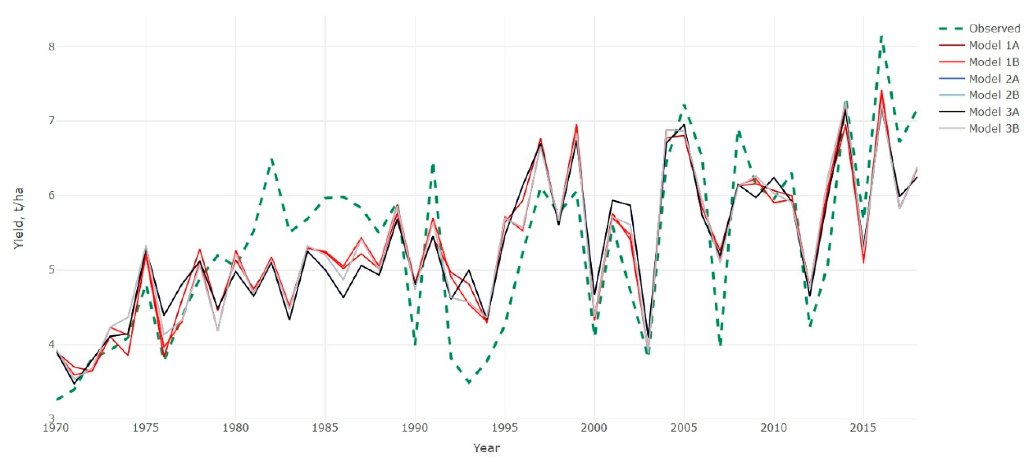
The table of regression results is a very important summary of the model specification assortment, but Figure 2 provides the graphical illustration of the model charts compared to the observed yields.
In general the predicted model specifications closely follow the observed annual aggregates. However, the deviations in the 1980s and in the mid-1990s can be attributed to the external influencing effects occurring over the transition period, for instance, political instability, transformation of farm structure, and other effects, all of which are implicitly addressed in the human impact and thus lower the year-to-year sensitivity of the models.
These models are used for estimating future corn yields as we make predictions with projected future weather. We either superpose the foreseen linear trend and account for persisting human impact in the future or disjoint the elevated CO2 effect from the human impact. We find the contribution of human impact about 80 kg/ha/year to increase corn yield, of which we consider ca. 8 kg/ha/year for elevated CO2 (see Section 2, [40,41]). We argue that elevated CO2 level is independent from human impact (it rather may be seen as a humanity impact), and therefore, we cover for the elevated CO2 in the future when no persisting human impact is assumed.
We show the results of both possible alternatives and assess future corn yields with and without persisting human impact. The sets of result figures are presented in the Supplementary Materials, together with an imposed linear trend on the annual aggregated yield outcomes (LT) (see Figures S2–S13). We find the most favorable climate projection of RCA-HadCM3Q0 (assumes the highest precipitation and the mildest GDD increase compared to other projections) only slightly decreasing in the future without continuous human impact. However, if we assume that human innovations will persist as much as in the past, we find the opposite directions of the trends. The preferential projection of RCA-HadCM3Q0 increases the most of all, by confirming that positive social and environmental effects reinforce each other. The charts exhibit that corn yields may reach the 12–16 t/ha level by the end of the century.
Here, we present the ensemble of the six climate projections collectively for all model specifications, together with the linear trend (LT) of the aggregated results (Figure 3 and Figure 4), to filter out the feasible differences between the RCMs and afford to assess the attainable distinctions between the models. The pairwise coloring of the graphs is entitled to help easier perception of the respective charts. In general, models with specification “A,” when the growing period is not divided into vegetative and reproductive growth phases, predict higher corn yields than models with specification ”B.” This suggests that, when more detailed model specification is applied, the predicted results show fairly identical and more robust results (see all “B” specifications). In other words, when we decrease the explanatory power of the set of independent variables, in Model 2A and Model 3A (compared also to Model 1A, not only to all “B” specifications), we find that the results of these two models go far beyond the rest.
All models confirm that climate change in general will have a negative impact on Hungarian corn yields. The compiled model charts from all projection outcomes confirm the great importance of sustaining competitiveness and improving farm efficiency. The comparison of the ensembles reveals that corn cropping systems are in real danger due to climate change, but it is not impossible to sustain a vivid corn production for future generations.
4. Conclusions
Overall, our approach of treating the increasing trend in historic corn yields is substantially different than that in the mainstream literature, where the driving force behind increasing corn yield has been labelled as either “technology development,” “technological change,” or “improving adaptation capacity,” and modelled with, e.g., linear time trend, state-specific quadratic time trends, or year-fixed effects. We argue to compile all these different terminologies into one complex issue that we may call human impact, which subsumes all unidentified effects that facilitate corn yield development. In our view, long-term climate-yield interactions can only be addressed when human impact is explicitly taken into account. In reality, not only weather-related factors determine corn production, but also farmers’ behavior, production conditions, political establishment, research and development, as well as technological capabilities, etc. The technical problem of identifying these effects separately lies in finding the proper proxies for these determinants, and therefore, researchers often overlook these issues and focus merely on quantifiable weather components; methodologically, the increasing level of CO2 in the anthropogenic impact, or at least an aftermath. For long-term prediction, we disjoined this secondary effect and superposed its positive impact on corn yield when only the effect of elevated CO2 is considered.
Furthermore, the given heterogeneity between farms or production areas is also often disregarded. This paper shows the importance of addressing time-invariant production factors, when historic yield evolution is modelled. We confirm that soil parameters are crucial in future crop yield assessments, as it certainly has some implications for modeling. We applied the REWB hybrid framework that allows a wider range of variable use than the gold standard FE models. In principle, REWB allows for hierarchical data structure and approves time-invariant covariate use. We suppose that such indicators of soil characteristics and other individual characteristics will favor increasing prominence for modeling purposes.
Altogether, we elaborated six model specifications. Three “A” and three “B” settings indicate whether the growing period is considered in its overall length or differentiate the major plant growth phases, the vegetative and reproductive phases, respectively. We find the separation very meaningful and reveal the relative importance of more precipitation and radiation in the vegetative phase. The identified squared terms that are designed to account for the nonlinear relationship between weather variables and corn yield are zero in most cases. This implies that, for a study area like Hungary, where both soil and climate are rather favorable to corn production (relatively small area is affected by inland water, and the probability of the extremely long heat waves is low), the use of squared terms may be omitted. The rest of the results are found to be in line with the general theory of corn yield assessments.
Regarding human impact, with all models we calculated between 77 and 81 kg/ha of average annual increase in corn yields for the past that we superposed for future predictions. This indicates that activities of farmers and rather supportive establishment may lead to persistent development of Hungarian corn production. We show the potential best and worst possible outcomes for Hungarian corn production in the light of climate change until 2100 based on bias-corrected RCM simulations.
We find evidence that the Hungarian corn cropping system is vulnerable in the long run, but sustaining human impact certainly has the potential to reverse the projected decreasing trend. Still, there is room for sustainable intensification for corn production in Hungary, where “reversing the curve” means calling to organized actions of policy makers, farmers, and agricultural cooperatives to carry out great investments in precision farming, large-scale irrigation infrastructure development to provide more suitable farming conditions.
Further research may consider a more detailed identification of the components of human impact and thus contribute to make more comprehensive predictions.
Supplementary Materials
The following are available online at https://www.mdpi.com/2071-1050/12/17/6784/s1, Table S1: The decadal mean and standard deviation of climate impact indicators for the selected RCMs. Figure S1: Spatial distribution of aggregated yield, P, NHD and GDD; Figure S2–S13: Graphical illustration of 6 different RCMs with and without Human Impact.
Author Contributions
T.A.M. and N.F. worked out the concept of the manuscript. The methodology and R analysis were carried out by T.A.M. The observed corn yield dataset was provided by A.Z.-N., the climate data was assembled and compiled by A.K. (Anna Kis) and A.K. (Anikó Kern). All authors have read and agreed to the published version of the manuscript.
Funding
The research was supported by the Széchenyi 2020 program, the European Regional Development Fund “Investing in your future,” the Hungarian Government (GINOP-2.3.2-15-2016-00028), the János Bolyai Research Scholarship of the Hungarian Academy of Sciences (grant No. BO/00088/ 18/4) and by the Hungarian Scientific Research Fund (FK-128709 and K-129118).
Conflicts of Interest
The authors declare no conflict of interest. The funders had no role in the design of the study; in the collection, analyses, or interpretation of data; in the writing of the manuscript, or in the decision to publish the results.
References
- Rosenzweig, C.; Parry, M.L. Potential impact of climate change on world food supply. Nature 1994, 367, 133–138. [Google Scholar] [CrossRef]
- Kaufmann, R.K.; Snell, S.E. A Biophysical Model of Corn Yield: Integrating Climatic and Social Determinants. Am. J. Agric. Econ. 1997, 79, 178–190. [Google Scholar] [CrossRef]
- Nelson, G.C.; van der Mensbrugghe, D.; Ahammad, H.; Blanc, E.; Calvin, K.; Hasegawa, T.; Havlik, P.; Heyhoe, E.; Kyle, P.; Lotze-Campen, H.; et al. Agriculture and climate change in global scenarios: Why don’t the models agree. Agric. Econ. 2014, 45, 85–101. [Google Scholar] [CrossRef]
- Müller, C.; Robertson, R.D. Projecting future crop productivity for global economic modeling. Agric. Econ. 2014, 45, 37–50. [Google Scholar] [CrossRef]
- Wiebe, K.; Lotze-Campen, H.; Sands, R.; Tabeau, A.; Van Der Mensbrugghe, D.; Biewald, A.; Bodirsky, B.; Islam, S.; Kavallari, A.; Mason-D’Croz, D.; et al. Climate change impacts on agriculture in 2050 under a range of plausible socioeconomic and emissions scenarios. Environ. Res. Lett. 2015, 10, 85010. [Google Scholar] [CrossRef]
- Lobell, D.B.; Field, C.B. Global scale climate–Crop yield relationships and the impacts of recent warming. Environ. Res. Lett. 2007, 2, 014002. [Google Scholar] [CrossRef]
- Lobell, D.B.; Burke, M.B. On the use of statistical models to predict crop yield responses to climate change. Agric. For. Meteorol. 2010, 150, 1443–1452. [Google Scholar] [CrossRef]
- Schlenker, W.; Hanemann, W.M.; Fisher, A.C.; Will, U.S. Agriculture Really Benefit from Global Warming? Accounting for Irrigation in the Hedonic Approach. Am. Econ. Rev. 2005, 95, 395–406. [Google Scholar] [CrossRef] [Green Version]
- Eurostat. Grain Maize and corn-cob-mix by Area, Production and Humidity. Available online: https://ec.europa.eu/eurostat/databrowser/bookmark/dcb7c23b-33a1-484f-b964-439a4eb37a4a?lang=en (accessed on 24 June 2020).
- Bouma, J.; Varallyay, G.; Batjes, N. Principal land use changes anticipated in Europe. Agric. Ecosyst. Environ. 1998, 67, 103–119. [Google Scholar] [CrossRef]
- Gnansounou, E. Production and use of lignocellulosic bioethanol in Europe: Current situation and perspectives. Bioresour. Technol. 2010, 101, 4842–4850. [Google Scholar] [CrossRef]
- Hernandez-Ramirez, G.; Brouder, S.M.; Smith, D.R.; Van Scoyoc, G.E. Nitrogen partitioning and utilization in corn cropping systems: Rotation, N source, and N timing. Eur. J. Agron. 2011, 34, 190–195. [Google Scholar] [CrossRef]
- UN Comtrade. Corn Export of Hungary. Available online: http://comtrade.un.org/api/get?max=500&type=C&freq=A&px=HS&ps=all&r=348&p=0&rg=2&cc=1005 (accessed on 24 June 2020).
- Biacs, P.; Kocsondi, C.; Dobos, G. Tasks of Hungarian Agriculture and Forestry Deriving from the Climate Change. Gazdálkodás 2003, 47, 4–18, (In Hungarian: A magyar mező- és erdőgazdaság feladatai a klímaváltozás tükrében). [Google Scholar]
- Máté, F.; Makó, A.; Sisák, I.; Szász, G. Talajaink Klímaérzékenysége, Talajföldrajzi Vonatkozások. In Talajvédelem, Talajtani Vándorgyűlés; Talajvédelmi Alapítvány: Nyíregyháza, Hungary, 2008; pp. 141–147. [Google Scholar]
- Bartholy, J.; Bozó, L.; Haszpra, L. Klímaváltozás—Klímaszcenáriók a Kárpát-Medence Térségére; Magyar Tudományos Akadémia és az Eötvös Loránd Tudományegyetem Meteorológiai Tanszéke: Budapest, Hungary, 2011; pp. 1–287. [Google Scholar]
- Kocsis, M.; Dunai, A.; Makó, A.; Farsang, A.; Mészáros, J. Estimation of the drought sensitivity of Hungarian soils based on corn yield responses. J. Maps 2020, 16, 148–154. [Google Scholar] [CrossRef]
- Kocsis, M.; Dunai, A.; Farsang, A.; Makó, A. Soil-specific Drought Sensitivity of Subregions of Hungary Based on Yield Reactions of Arable Crops. Földrajzi Közlemények 2018, 142, 89–101. [Google Scholar]
- Pinke, Z.; Decsi, B.; Kozma, Z.; Vári, Á.; Lövei, G.L. A spatially explicit analysis of wheat and maize yield sensitivity to changing groundwater levels in Hungary, 1961–2010. Sci. Total Environ. 2020, 715, 136555. [Google Scholar] [CrossRef] [PubMed]
- Kovács, G.J.; Németh, T.; Ritchie, J.T. Testing simulation models for the assessment of crop production and nitrate leaching in Hungary. Agric. Syst. 1995, 49, 385–397. [Google Scholar] [CrossRef]
- Fodor, N.; Pásztor, L.; Németh, T. Coupling the 4M crop model with national geo-databases for assessing the effects of climate change on agro-ecological characteristics of Hungary. Int. J. Digit. Earth 2014, 7, 391–410. [Google Scholar] [CrossRef]
- Micskei, G.; Fodor, N.; Márton, L.; Bónis, P.; Árendás, T. Using long-term field experiment data to prepare a crop simulation model for climate impact studies. Appl. Ecol. Environ. Res. 2016, 14, 263–280. [Google Scholar] [CrossRef]
- Lobell, D.B.; Asseng, S. Comparing estimates of climate change impacts from process-based and statistical crop models. Environ Res. Lett. 2017, 12, 015001. [Google Scholar] [CrossRef]
- Challinor, A.J.; Müller, C.; Asseng, S.; Deva, C.; Nicklin, K.J.; Wallach, D.; Vanuytrecht, E.; Whitfield, S.; Ramirez-Villegas, J.; Koehler, A.-K. Improving the use of crop models for risk assessment and climate change adaptation. Agric. Syst. 2018, 159, 296–306. [Google Scholar] [CrossRef]
- Raksapatcharawong, M.; Veerakachen, W.; Homma, K.; Maki, M.; Oki, K. Satellite-Based Drought Impact Assessment on Rice Yield in Thailand with SIMRIW−RS. Remote Sens. 2020, 12, 2099. [Google Scholar] [CrossRef]
- Tewes, A.; Hoffmann, H.; Krauss, G.; Schäfer, F.; Kerkhoff, C.; Gaiser, T. New Approaches for the Assimilation of LAI Measurements into a Crop Model Ensemble to Improve Wheat Biomass Estimations. Agronomy 2020, 10, 446. [Google Scholar] [CrossRef] [Green Version]
- Cammarano, D.; Holland, J.; Ronga, D. Spatial and Temporal Variability of Spring Barley Yield and Quality Quantified by Crop Simulation Model. Agronomy 2020, 10, 393. [Google Scholar] [CrossRef] [Green Version]
- Ewert, E.; Rötter, R.P.; Bindi, M.; Webber, H.; Trnka, M.; Kersebaum, K.C.; Olesen, J.E.; van Ittersum, M.K.; Janssen, S.; Rivington, M.; et al. Crop modelling for integrated assessment of risk to food production from climate change. Environ. Model. Softw. 2015, 7, 287–303. [Google Scholar] [CrossRef]
- Lobell, D.B.; Gourdji, S.M. The influence of climate change on global crop productivity. Plant Physiol. 2012, 160, 1686–1697. [Google Scholar] [CrossRef] [Green Version]
- Auffhammer, M.; Ramanathan, V.; Vincent, J.R. Integrated model shows that atmospheric brown clouds and greenhouse gases have reduced rice harvests in India. Proc. Natl. Acad. Sci. USA 2006, 103, 19668–19672. [Google Scholar] [CrossRef] [Green Version]
- Auffhammer, M.; Ramanathan, V.; Vincent, J.R. Climate change, the monsoon, and rice yield in India. Clim. Chang. 2012, 111, 411–424. [Google Scholar] [CrossRef]
- Anselin, L. Spatial Effects in Econometric Practice in Environmental and Resource Economics. Am. J. Agric. Econ. 2001, 83, 705–710. [Google Scholar] [CrossRef]
- Hawkins, E.; Fricker, T.E.; Challinor, A.J.; Ferro, C.A.T.; Ho, C.K.; Osborne, T.M. Increasing influence of heat stress on French maize yields from the 1960s to the 2030s. Glob. Chang. Biol. 2013, 19, 937–947. [Google Scholar] [CrossRef] [Green Version]
- Moore, F.C.; Lobell, D.B. Adaptation potential of European agriculture in response to climate change. Nat. Clim. Chang. 2014, 4, 610–614. [Google Scholar] [CrossRef]
- Moore, F.C.; Lobell, D.B. The fingerprint of climate trends on european crop yields. Proc. Natl. Acad. Sci. USA 2015, 112, 2970–2975. [Google Scholar] [CrossRef] [PubMed] [Green Version]
- Hertel, T.W.; Lobell, D.B. Agricultural adaptation to climate change in rich and poor countries: Current modeling practice and potential for empirical contributions. Energy Econ. 2014, 46, 562–575. [Google Scholar] [CrossRef] [Green Version]
- Schlenker, W.; Roberts, M.J.; Smith, V.K.; Schlenker3-, W.; Roberts6, M.J. Nonlinear temperature effects indicate severe damages to U.S. crop yields under climate change. Proc. Natl. Acad. Sci. USA 2009, 106, 15594–15598. [Google Scholar] [CrossRef] [PubMed] [Green Version]
- Roberts, M.J.; Schlenker, W.; Eyer, J. Agronomic Weather Measures in Econometric Models of Crop Yield with Implications for Climate Change. Am. J. Agric. Econ. 2013, 95, 236–243. [Google Scholar] [CrossRef]
- Leakey, A.D.B.; Ainsworth, E.A.; Bernacchi, C.J.; Rogers, A.; Long, S.P.; Ort, D.R. Elevated CO2 effects on plant carbon, nitrogen, and water relations: Six important lessons from FACE. J. Exp. Bot. 2009, 60, 2859–2876. [Google Scholar] [CrossRef]
- Weigel, H.J.; Manderscheid, R. FACE with Crops: Data for Climate Change Impact Models. Thünen a la Carte 2016, 4a, 1–6. [Google Scholar]
- Castaño-Sánchez, J.P.; Rotz, C.A.; Karsten, H.D.; Kemanian, A.R. Elevated atmospheric carbon dioxide effects on maize and alfalfa in the Northeast US: A comparison of model predictions and observed data. Agric. For. Meteorol. 2020, 291, 108093. [Google Scholar] [CrossRef]
- Dobor, L.; Barcza, Z.; Hlásny, T.; Havasi, Á.; Horváth, F.; Ittzés, P.; Bartholy, J. Bridging the gap between climate models and impact studies: The FORESEE Database. Geosci. Data J. 2015, 2, 1–11. [Google Scholar] [CrossRef]
- Kern, A.; Dobor, L.; Horváth, F.; Hollós, R.; Márta, G.; Barcza, Z. Hungarian: FORESEE: Egy Publikus Meteorológiai Adatbázis a Kárpát-Medence Tágabb Térségére (Extended Absrtract). Az Elmélet és a Gyakorlat Találkozása a Térinformatikában; Szerk.: Molnár Vanda Éva. Debrecen Egyetemi Kiadó, 2019. Available online: http://giskonferencia.unideb.hu/arch/GIS_Konf_kotet_2019.pdf (accessed on 20 August 2020).
- Cornes, R.C.; van der Schrier, G.; van den Besselaar, E.J.M.; Jones, P.D. An Ensemble Version of the E-OBS Temperature and Precipitation Data Sets. J. Geophys. Res. Atmos. 2018, 123, 9391–9409. [Google Scholar] [CrossRef] [Green Version]
- van der Linden, P.; Mitchell, J.F. ENSEMBLES: Climate Change and Its Impacts: Summary of Research and Results From the ENSEMBLES Project; Met Office Hadley Centre: London, UK, 2009; p. 160.
- Nakicenovic, N.; Swart, R. Emissions Scenarios. A special report of IPCC Working Group III; Pacific Northwest National Laboratory: Richland, WA, USA, 2000. [Google Scholar]
- Hawkins, E.; Sutton, R. The potential to narrow uncertainty in projections of regional precipitation change. Clim. Dyn. 2011, 37, 407–418. [Google Scholar] [CrossRef]
- Kern, A.; Marjanović, H.; Barcza, Z. Evaluation of the Quality of NDVI3g Dataset against Collection 6 MODIS NDVI in Central Europe between 2000 and 2013. Remote Sens. 2016, 8, 955. [Google Scholar] [CrossRef] [Green Version]
- Thornton, P.E.; Hasenauer, H.; White, M.A. Simultaneous estimation of daily solar radiation and humidity from observed temperature and precipitation: An application over complex terrain in Austria. Agric. For. Meteorol. 2000, 104, 255–271. [Google Scholar] [CrossRef]
- Deschênes, O.; Greenstone, M. The Economic Impacts of Climate Change: Evidence from Agricultural Output and Random Fluctuations in Weather. Am. Econ. Rev. 2007, 97, 354–385. [Google Scholar] [CrossRef] [Green Version]
- Baylis, K.; Paulson, N.D.; Piras, G. Spatial Approaches to Panel Data in Agricultural Economics: A Climate Change Application. J. Agric. Appl. Econ. 2011, 43, 325–338. [Google Scholar] [CrossRef] [Green Version]
- Deschênes, O.; Greenstone, M. The Economic Impacts of Climate Change: Evidence from Agricultural Output and Random Fluctuations in Weather: Reply. Am. Econ. Rev. 2012, 102, 3761–3773. [Google Scholar] [CrossRef]
- Pásztor, L.; Laborczi, A.; Takács, K.; Szatmári, G.; Bakacsi, Z.; Szabó, J. DOSoReMI as the national implementation of GlobalSoilMap for the territory of Hungary. In GlobalSoilMap—Digital Soil Mapping from Country to Globe; CRC Press: London, UK, 2018; pp. 17–22. [Google Scholar]
- Schurer, S.; Yong, J. Personality, Well-Being and the Marginal Utility of Income: What Can We Learn from Random Coefficient Models? Working Paper 01/2012; School of Economics and Finance, Victoria University of Wellington: Wellington, New Zealand, 2012. [Google Scholar]
- Molenberghs, G.; Verbeke, G. A review on linear mixed models for longitudinal data, possibly subject to dropout. Stat. Model. 2001, 1, 235–269. [Google Scholar] [CrossRef] [Green Version]
- Molenberghs, G.; Verbeke, G. Models for discrete Longitudinal Data; Springer: New York, NY, USA, 2005. [Google Scholar] [CrossRef]
- Beck, N.; Katz, J.N. Random Coefficient Models for Time-Series—Cross-Section Data: Monte Carlo Experiments. Polit. Anal. 2007, 15, 182–195. [Google Scholar] [CrossRef]
- Jones, K.; Johnston, R.J.; Pattie, C.J. People, Places and Regions: Exploring the Use of Multi-Level Modelling in the Analysis of Electoral Data. Br. J. Polit. Sci. 1992, 22, 343–380. [Google Scholar] [CrossRef]
- Lewis, D.J.; Barham, B.L.; Zimmerer, K.S. Spatial Externalities in Agriculture: Empirical Analysis, Statistical Identification, and Policy Implications. World Dev. 2008, 36, 1813–1829. [Google Scholar] [CrossRef] [Green Version]
- Lewis, D.J.; Barham, B.L.; Robinson, B. Are There Spatial Spillovers in the Adoption of Clean Technology? The Case of Organic Dairy Farming. Land Econ. 2011, 87, 250–267. [Google Scholar] [CrossRef]
- Bell, A.; Jones, K. Explaining Fixed Effects: Random Effects Modeling of Time-Series Cross-Sectional and Panel Data. Polit. Sci. Res. Methods 2015, 3, 133–153. [Google Scholar] [CrossRef] [Green Version]
- Bell, A.; Jones, K.; Fairbrother, M. Understanding and misunderstanding group mean centering: A commentary on Kelley et al.’s dangerous practice. Qual. Quant. 2018, 52, 2031–2036. [Google Scholar] [CrossRef] [PubMed] [Green Version]
- Bell, A.; Fairbrother, M.; Jones, K. Fixed and random effects models: Making an informed choice. Qual. Quant. 2019, 53, 1051–1074. [Google Scholar] [CrossRef] [Green Version]
- Mundlak, Y. On the Pooling of Time Series and Cross Section Data. Econometrica 1978, 46, 69–85. [Google Scholar] [CrossRef]
- Mundlak, Y. Models with Variable Coefficients: Integration and Extension. Ann. Insee 1978, 30/31, 483–509. [Google Scholar] [CrossRef]
- Howard, A.L. Leveraging Time-Varying Covariates to Test Within- and Between-Person Effects and Interactions in the Multilevel Linear Model. Emerg. Adulthood 2015, 3, 400–412. [Google Scholar] [CrossRef]
- Croissant, Y.; Millo, G. Panel Data Econometrics in R: The plm Package. J. Stat. Softw. 2008, 27. [Google Scholar] [CrossRef] [Green Version]
- Bates, D.; Mächler, M.; Bolker, B.; Walker, S. Fitting Linear Mixed-Effects Models Using lme4. J. Stat. Softw. 2015, 67, 1–48. [Google Scholar] [CrossRef]
- Hamner, B.; Frasco, M.; LeDell, E. Metrics: Evaluation Metrics for Machine Learning. Available online: https://CRAN.R-project.org/package=Metrics (accessed on 20 August 2020).
- Sievert, C. Interactive Web-Based Data Visualization with R, Plotly, and Shiny; CRC Press: London, UK, 2020; ISBN 0429824203. [Google Scholar]
- Spanos, A. Revisiting the omitted variables argument: Substantive vs. statistical adequacy. J. Econ. Methodol. 2006, 13, 179–218. [Google Scholar] [CrossRef]
Figure 1.
The historic evolution of Hungarian and European corn yields (1970–2018).

Figure 2.
Observed and modeled corn yields in Hungary (1970–2018).

Figure 3.
Ensemble of six RCM simulations for all model specifications with persisting human impact.
Figure 3.
Ensemble of six RCM simulations for all model specifications with persisting human impact.

Figure 4.
Ensemble of six RCM simulations for all model specifications without persisting human impact.
Figure 4.
Ensemble of six RCM simulations for all model specifications without persisting human impact.


Table 1.
Summary table of performed variable structures in each model.
| Variables | Model 1A | Model 1B | Model 2A | Model 2B | Model 3A | Model 3B |
|---|---|---|---|---|---|---|
| GDD | + | + | + | |||
| GDD2 | + | + | + | |||
| GDDVEGETATIVE | + | + | + | |||
| GDD2VEGETATIVE | + | + | + | |||
| GDDREPRODUCTIVE | + | + | + | |||
| GDD2REPRODUCTIVE | + | + | + | |||
| RADVEGETATIVE | + | + | ||||
| RAD2VEGETATIVE | + | + | ||||
| RADREPRODUCTIVE | + | + | ||||
| RAD2REPRODUCTIVE | + | + | ||||
| P | + | + | + | |||
| P2 | + | + | + | |||
| PVEGETATIVE | + | + | + | |||
| P2VEGETATIVE | + | + | + | |||
| PREPRODUCTIVE | + | + | + | |||
| P2REPRODUCTIVE | + | + | + | |||
| NHD | + | + | + | + | + | + |
| SOM | + | + | + | + | ||
| pH | + | + | + | + | ||
| Sand | + | + | + | + |
Table 2.
Regression Results of REWB models from a Variety of Panel Specifications.
| Model 1A | Model 1B | Model 2A | Model 2B | Model3A | Model3B | |||||||||||||
|---|---|---|---|---|---|---|---|---|---|---|---|---|---|---|---|---|---|---|
| Predictors | Estimates | SE | p | Estimates | SE | p | Estimates | SE | p | Estimates | SE | p | Estimates | SE | p | Estimates | SE | p |
| (Intercept) | 303.348 | 218.238 | 0.165 | 200.941 | 207.542 | 0.333 | 0.756 | 5.060 | 0.881 | −32.381 | 13.771 | 0.019 | −0.537 | 5.362 | 0.920 | −52.862 | 15.829 | 0.001 |
| Time trend | 0.081 | 0.001 | <0.001 | 0.079 | 0.001 | <0.001 | 0.078 | 0.001 | <0.001 | 0.077 | 0.001 | <0.001 | 0.078 | 0.001 | <0.001 | 0.077 | 0.001 | <0.001 |
| GDD within | 0.005 | 0.000 | <0.001 | 0.006 | 0.000 | <0.001 | 0.006 | 0.000 | <0.001 | |||||||||
| GDD between | 0.009 | 0.008 | 0.231 | −0.010 | 0.007 | 0.170 | −0.015 | 0.008 | 0.063 | |||||||||
| GDD2 within | 0.000 | 0.000 | <0.001 | 0.000 | 0.000 | <0.001 | 0.000 | 0.000 | <0.001 | |||||||||
| GDD2 between | 0.000 | 0.000 | 0.551 | 0.000 | 0.000 | 0.032 | 0.000 | 0.000 | 0.009 | |||||||||
| RADVEG within | 0.097 | 0.004 | <0.001 | 0.068 | 0.004 | <0.001 | ||||||||||||
| RADVEG between | 0.051 | 0.290 | 0.862 | −0.947 | 0.322 | 0.003 | ||||||||||||
| RAD2VEG within | 0.000 | 0.000 | <0.001 | 0.000 | 0.000 | <0.001 | ||||||||||||
| RAD2VEG between | 0.000 | 0.000 | 0.935 | 0.000 | 0.000 | 0.004 | ||||||||||||
| RADREP within | −0.003 | 0.004 | 0.490 | −0.022 | 0.004 | <0.001 | ||||||||||||
| RADREP between | −0.485 | 0.179 | 0.007 | 0.417 | 0.210 | 0.047 | ||||||||||||
| RAD2REP within | 0.000 | 0.000 | 0.058 | 0.000 | 0.000 | <0.001 | ||||||||||||
| RAD2REP between | 0.000 | 0.000 | 0.005 | 0.000 | 0.000 | 0.065 | ||||||||||||
| P within | 0.008 | 0.000 | <0.001 | 0.009 | 0.000 | <0.001 | 0.009 | 0.000 | <0.001 | |||||||||
| P between | −0.004 | 0.015 | 0.770 | 0.026 | 0.014 | 0.061 | 0.061 | 0.015 | <0.001 | |||||||||
| P2 within | 0.000 | 0.000 | <0.001 | 0.000 | 0.000 | <0.001 | 0.000 | 0.000 | <0.001 | |||||||||
| P2 between | 0.000 | 0.000 | 0.895 | 0.000 | 0.000 | 0.102 | 0.000 | 0.000 | <0.001 | |||||||||
| NHD within | −0.069 | 0.001 | <0.001 | −0.069 | 0.001 | <0.001 | −0.074 | 0.001 | <0.001 | −0.071 | 0.001 | <0.001 | −0.074 | 0.001 | <0.001 | −0.071 | 0.001 | <0.001 |
| NHD between | −0.099 | 0.020 | <0.001 | −0.027 | 0.020 | 0.181 | −0.070 | 0.014 | <0.001 | 0.027 | 0.017 | 0.112 | −0.044 | 0.015 | 0.003 | 0.079 | 0.020 | <0.001 |
| SOM | 0.245 | 0.073 | 0.001 | 0.291 | 0.068 | <0.001 | 0.156 | 0.073 | 0.033 | 0.149 | 0.075 | 0.046 | ||||||
| pH | 0.315 | 0.064 | <0.001 | 0.251 | 0.060 | <0.001 | 0.285 | 0.067 | <0.001 | 0.220 | 0.067 | 0.001 | ||||||
| Sand | −0.015 | 0.002 | <0.001 | −0.014 | 0.002 | <0.001 | −0.016 | 0.002 | <0.001 | −0.016 | 0.002 | <0.001 | ||||||
| GDDVEG within | −0.007 | 0.001 | <0.001 | −0.004 | 0.001 | <0.001 | −0.004 | 0.001 | <0.001 | |||||||||
| GDDVEG between | −0.189 | 0.095 | 0.046 | −0.223 | 0.104 | 0.031 | −0.343 | 0.122 | 0.005 | |||||||||
| GDD2VEG within | 0.000 | 0.000 | <0.001 | 0.000 | 0.000 | <0.001 | 0.000 | 0.000 | <0.001 | |||||||||
| GDD2VEG between | 0.000 | 0.000 | 0.106 | 0.000 | 0.000 | 0.064 | 0.000 | 0.000 | 0.013 | |||||||||
| GDDREP within | 0.016 | 0.001 | <0.001 | 0.018 | 0.001 | <0.001 | 0.018 | 0.001 | <0.001 | |||||||||
| GDDREP between | 0.182 | 0.073 | 0.012 | 0.196 | 0.080 | 0.015 | 0.300 | 0.094 | 0.001 | |||||||||
| GDD2REP within | 0.000 | 0.000 | <0.001 | 0.000 | 0.000 | <0.001 | 0.000 | 0.000 | <0.001 | |||||||||
| GDD2REP between | 0.000 | 0.000 | 0.030 | 0.000 | 0.000 | 0.030 | 0.000 | 0.000 | 0.004 | |||||||||
| PVEG within | 0.015 | 0.001 | <0.001 | 0.018 | 0.000 | <0.001 | 0.018 | 0.000 | <0.001 | |||||||||
| PVEG between | −0.182 | 0.030 | <0.001 | −0.132 | 0.033 | <0.001 | −0.191 | 0.038 | <0.001 | |||||||||
| P2VEG within | 0.000 | 0.000 | <0.001 | 0.000 | 0.000 | <0.001 | 0.000 | 0.000 | <0.001 | |||||||||
| P2VEG between | 0.001 | 0.000 | <0.001 | 0.000 | 0.000 | <0.001 | 0.001 | 0.000 | <0.001 | |||||||||
| PREP within | 0.001 | 0.000 | 0.130 | −0.002 | 0.000 | <0.001 | −0.002 | 0.000 | <0.001 | |||||||||
| PREP between | 0.045 | 0.017 | 0.009 | 0.030 | 0.017 | 0.079 | 0.077 | 0.020 | <0.001 | |||||||||
| P2REP within | 0.000 | 0.000 | 0.091 | 0.000 | 0.000 | <0.001 | 0.000 | 0.000 | <0.001 | |||||||||
| P2REP between | 0.000 | 0.000 | 0.043 | 0.000 | 0.000 | 0.173 | 0.000 | 0.000 | <0.001 | |||||||||
| σ2 | 1.08 | 1.05 | 1.13 | 1.06 | 1.13 | 1.06 | ||||||||||||
| N | 1104 ID | 1104 ID | 1104 ID | 1104 ID | 1104 ID | 1104 ID | ||||||||||||
| Observations | 54,096 | 54,096 | 54,096 | 54,096 | 54,096 | 54,096 | ||||||||||||
| Marginal R2/Cond R2 | 0.370/0.711 | 0.396/0.710 | 0.356/0.673 | 0.369/0.701 | 0.303/0.667 | 0.309/0.709 | ||||||||||||
| AIC/BIC | 163,312/163,552 | 161,855/162,166 | 165,734/165,903 | 162,580/162,820 | 165,978/166,120 | 162,806/163,020 | ||||||||||||
| RMSE | 1.0229 | 1.0083 | 1.0465 | 1.0143 | 1.0461 | 1.0136 | ||||||||||||
Note: Significant estimates are shown in bold.
© 2020 by the authors. Licensee MDPI, Basel, Switzerland. This article is an open access article distributed under the terms and conditions of the Creative Commons Attribution (CC BY) license (http://creativecommons.org/licenses/by/4.0/).
Share and Cite
MDPI and ACS Style
Marton, T.A.; Kis, A.; Zubor-Nemes, A.; Kern, A.; Fodor, N. Human Impact Promotes Sustainable Corn Production in Hungary. Sustainability 2020, 12, 6784. https://doi.org/10.3390/su12176784
AMA Style
Marton TA, Kis A, Zubor-Nemes A, Kern A, Fodor N. Human Impact Promotes Sustainable Corn Production in Hungary. Sustainability. 2020; 12(17):6784. https://doi.org/10.3390/su12176784
Chicago/Turabian StyleMarton, Tibor András, Anna Kis, Anna Zubor-Nemes, Anikó Kern, and Nándor Fodor. 2020. "Human Impact Promotes Sustainable Corn Production in Hungary" Sustainability 12, no. 17: 6784. https://doi.org/10.3390/su12176784
Note that from the first issue of 2016, this journal uses article numbers instead of page numbers. See further details here.