Primary Pollutants and Air Quality Analysis for Urban Air in China: Evidence from Shanghai

Abstract

In recent years, China’s urban air pollution has caused widespread concern in the academic world. As one of China’s economic and financial centers and one of the most densely populated cities, Shanghai ranks among the top in China in terms of per capita energy consumption per unit area. Based on the Shanghai Energy Statistical Yearbook and Shanghai Air Pollution Statistics, we have systematically analyzed Shanghai’s atmospheric pollutants from three aspects: Primary pollutants, pollutants changing trends, and fine particulate matter. The comprehensive pollution index analysis method, the grey correlation analysis method, and the Euclid approach degree method are used to evaluate and analyze the air quality in Shanghai. The results have shown that Shanghai’s primary pollutants are PM_2.5 and O₃, and the most serious air pollution happens during the first half of the year, particularly in the winter. This is because it is the peak period of industrial energy use, and residential heating will also lead to an increase in energy consumption. Furthermore, by studying the particulate pollutants of PM_2.5 and PM₁₀, we clearly disclosed the linear correlation between PM_2.5 and PM₁₀ concentrations in Shanghai which varies seasonally.

1. Introduction

In recent years, with China’s rapid economic development, consumption of fossil energy has also grown rapidly, and its air quality, especially in cities, has deteriorated drastically, causing a significant negative impact on people’s health as well as climate change [1,2,3,4]. It has been realized that the scope and severity of urban air pollution are affected by the nature of air pollutants and pollution sources [5], weather conditions [6,7,8], as well as properties of the land surface [9,10,11]. These factors are influenced by natural factors (such as air pressure [12], temperature [13], wind direction and speed [14], etc.), but human factors (such as industrial waste gas emissions [15], domestic coal combustion [16,17], automobile exhaust emissions [18], etc.) have a greater impact on the urban air quality. At the same time, human activities also affect natural factors to a certain extent, and a considerable part of the human factors come from the unreasonable consumption of primary energy and secondary energy. The energy consumption structure is closely connected to the industrial structure [19,20]. The current industrial structure with high consumption and low output has further resulted in the deterioration of air quality.

Shanghai is China’s largest industrial city and an energy-consuming city, with a per capita energy consumption and unit area energy consumption much higher than the national average. Its total energy consumption has increased from 106.71 million tons of standard coal in 2010 to 117.12 million tons of standard coal in 2016 [21], while the total energy consumption nationwide was 4.36 billion tons of standard coal in 2016 [22], which means Shanghai’s total energy consumption accounted for 3% of the total energy consumption of 338 cities in China. What comes with such high energy consumption density is the deterioration of Shanghai’s urban environment. According to the data in the Shanghai Environmental Condition Bulletin, the number of days with good air quality was only 275 in 2017, with an Air Quality Index (AQI) good rate of 75.3% [23]. The requirement of continuous economic growth, the increasing consumption of energy and resources, and the continuous deterioration of air quality have brought tremendous pressure and severe challenges to the sustained and stable development of Shanghai’s economy and society.

In order to meet the requirements of air quality under the new circumstances, in 2012, China issued a new national ambient air quality standard (GB 3095-2012), which clarified the calculation method of AQI [24]:

First, calculate the Individual Air Quality Index of certain pollutant ($IAQ{I}_P$):

$$IAQ{I}_P=\frac{IAQ{I}_{Hi}-IAQ{I}_{Lo}}{B{P}_{Hi}-B{P}_{Lo}}\left(C_P-B{P}_{Lo}\right)+IAQ{I}_{Lo}$$

(1)

In the equation above, $C_P$ represents the mass concentration of pollutant P; $B{P}_{Hi}$ is the higher threshold of pollutant concentration near $C_P$ corresponding to the specified IAQI (Individual Air Quality Index) regulated by government policy; $B{P}_{Lo}$ is the lower threshold of pollutant concentration near $C_P$ regulated by the government; $IAQ{I}_{Hi}$ is the corresponding IAQI to $B{P}_{Hi}$; while $IAQ{I}_{Lo}$ is the corresponding IAQI to $B{P}_{Lo}$.

Then, take the largest number from all $IAQ{I}_P$ to calculate the $AQI$:

$$AQI=max\left\{IAQ{I}_1, IAQ{I}_2, IAQ{I}_3, \cdots , IAQ{I}_n\right\}$$

(2)

In 2013, the first year the new ambient air quality standard was implemented, the air quality monitoring and evaluation work of Shanghai started to follow the new standards including the Ambient Air Quality Standards (GB3095-2012) and the Technical Regulation on Ambient Air Quality Index (HJ 633-2012) [25]. This was a great opportunity to study the impact of Shanghai’s energy consumption structure on its air quality, accelerate the optimization of Shanghai’s energy consumption structure, and build an energy-saving society, which is of great significance to the construction of an international city.

Currently, studies on related fields mainly focus on three aspects. The first is the analysis of fine particle pollution and its impact on atmospheric visibility in cities. The second is the concentration feature and chemical composition of air pollutants. The third is the description of emission factors of air pollutants.

Li et al. (2019) studied the meteorological conditions of the severe haze weather that frequently occurred in North China and concluded two main reasons for the decrease in visibility [26]. The first is the influence of meteorological conditions such as atmospheric currents, and the second is the change in the average astigmatism coefficient caused by the absorption and scattering of light due to fine particles and major air pollutants [26]. Golly et al. [27] (2019) conducted experiments on the chemical characterization of PM_2.5 particles in five rural areas of France, and conducted chemical analysis on the samples every 6 days, including their organic carbon (OC), elemental carbon (EC), ion species, etc. The results showed that wood combustion had made high contributions to the organic carbon (OC), and in some rural areas, the contribution rate of wood combustion to OC could be as high as 90% in winters; the contribution of terrestrial protozoa organic components was also significant in summers and autumns, with a monthly PM_2.5 contribution rate of 4.5–9.5% [27]. Ryu et al. (2019) studied the PM (Particulate Matter) removal effect of plant evapotranspiration by using the PM removal performance of five plants and the relative humidity (RH) in a closed chamber as control parameters. The results showed that under effective transpiration, honeysuckle had higher efficiency for aerosol PM_2.5 removal [28].

At the same time, relevant departments of different countries have also formulated different emission inventories in response to air pollution. The U.S. Environmental Protection Agency (EPA) has established the emission inventory for pollutants through direct measurements of power plants stacks, which provides emission measurements that have an error of less than 2% [29]. The establishment of this emission inventory has provided valuable guidance to the study of the impact of energy consumption on the atmospheric environment. The European Environment Agency (EEA) has established an emission inventory for 30 countries and regions including France and Germany, which covers 8 pollutants (NO_x, SO₂, CO, NH₃, CH₄, N₂O, CO₂, NMVOC) [30]. The study of the emission inventory in Asia started relatively late. Ohara et al. established an emission inventory of Asia from 1980–2020, in which the pollutants mainly come from energy consumption such as the combustion of fossil fuel and biomass fuel for industrial, power, transportation and civil use [31]. This is a relatively comprehensive emission inventory for Asia so far. Meanwhile, Korea and Japan are expected to have their own emission inventory [32,33,34,35].

In current studies, there is a lack of systematic and quantitative research on the migration characteristics of urban air pollutants under the influence of energy consumption and estimation of pollutants produced by energy consumption. Therefore, it is important to analyze the characteristics of urban air pollution by relating to the energy consumption needs of Shanghai as a mega-city in its economic and social development, in order to improve its air quality as well as the life quality of its residents. This paper has adopted the Comprehensive Pollution Index Method, the Improved Grey Relational Degree Method, and the Euclid Approach Degree Method to evaluate the air quality of Shanghai, and systematically analyzed the changing pattern and correlation of fine particle pollutants (PM_2.5 and PM₁₀) in Shanghai, in order to achieve innovations as following:

(1) By introducing the pollution index analysis method, the grey correlation analysis method, and the Euclid approach degree method comprehensively, we hope to overcome their respective deficiencies and make new additions to existing research methods.

(2) By further discussing the changing pattern and correlation of the fine particle pollutants (PM_2.5 and PM₁₀), we hope to provide new evidence of the interrelationship between major atmospheric pollutants in China.

In the following parts of this paper: Section 2 introduces the backgrounds and methods of this paper and introduces three study methods. Section 3 uses the three methods to calculate and evaluate the air quality of Shanghai from 1 November 2017 to 31 October 2018. Based on the above assessment, Section 4 further discusses the changing pattern and correlation of the fine particle pollutants (PM_2.5 and PM₁₀) in Shanghai during the study period. Finally, Section 5 provides conclusions of this paper.

2. Materials and Methods

2.1. Introduction of China’s AQI System

In order to meet the public’s increasing requirement of air quality, and objectively reflect the air pollution situation in China at the same time, in the first half of 2012, the Ministry of Environmental Protection of China issued the Technical Regulation on Ambient Air Quality Index (HJ 633-2012) to replace the previous Air Pollution Index (API). The pollutants covered by this new standard increased to 6 items (SO₂, NO₂, PM₁₀, PM_2.5, O₃, and CO). The AQI is divided into six levels, which represent superior air quality, good air quality, mild pollution, moderate pollution, heavy pollution, and severe pollution respectively from the highest to the lowest level. The corresponding Air Quality Indexes are: Level I—0–50, Level II—50–100, Level III—101–150, Level IV—151–200, Level V—201–300, and Level VI—above 300 [25]. See

Table 1. Air Quality Index Range and corresponding impact.

Air Quality Index Range	Air Quality Level	Air Quality Category	Representative Color	Impacts on Human Health and Recommended Actions
0–50	Level I	Superior	Green	The air quality is satisfactory. There is basically no air pollution, and no impact on human activities.
51–100	Level II	Good	Yellow	The air quality is acceptable. There are certain air pollutants that may cause health issues to a small number of people who should reduce outdoor activities.
101–150	Level III	Mild Pollution	Orange	Symptoms in susceptible people would intensify, and healthy people would show irritation symptoms. Elderly people and children should avoid long hours of high-intensity outdoor exercises.
151–200	Level IV	Moderate Pollution	Red	Symptoms in susceptible people would further intensify, and the breathing of healthy people would be affected. Elderly people and children should avoid outdoor sports.
201–300	Level V	Heavy Pollution	Purple	Ordinary people would show symptoms. Elderly people and children should avoid outdoor sports. The general population should reduce outdoor activities.
>300	Level VI	Severe Pollution	Maroon	Obvious and strong symptoms would appear, and all groups of people should avoid outdoor activities.

for details of each level.

2.2. Overview of Shanghai Air Quality

The main air pollutants in Shanghai include SO₂, NO₂, PM₁₀, PM_2.5, O₃, and CO. According to the data released by the Shanghai Environmental Hotline, the main pollutants published before 2012 include SO₂, NO₂, and PM₁₀. Since 2012, PM_2.5, O₃, and CO have been added to the published main pollutants [36].

Taking 2017 as an example, according to the AQI evaluation, the number of days with superior and good air quality in Shanghai was 275, which was 1 day less than that in 2016. The good AQI rate was 75.3%, which was 0.1% point lower than that of 2016. Overall speaking, there were 58 days with superior air quality, 217 days with good air quality, 71 days with mild pollution, 17 days with moderate air pollution, and 2 days with heavy pollution. The number of days with heavy pollution was the same with that in 2016. In those 90 days with air pollution, there were 52 days in which ozone (O₃) was the primary air pollutant (the maximum IAQI air pollutant when AQI is greater than 50 [25]), accounting for 57.8% of the pollution days; there were 23 days in which fine particles (PM_2.5) was the primary air pollutant, accounting for 25.6% of the pollution days; there were 12 days in which nitrogen dioxide (NO₂) was the primary air pollutant, accounting for 13.3% of the pollution days; there were 2 days in which inhalable particles (PM₁₀) was the primary air pollutant (due to the transportation of sand dust), accounting for 2.2% of the pollution days; there was 1 day in which PM_2.5 and NO₂ were the primary air pollutants, accounting for 1.1% of the pollution days [23].

In 2017, the annual average concentration of PM_2.5 in Shanghai was 39 μg/m³, which exceeded the Level II national air quality standard of 4 μg/m³ and decreased by 13.3% and 37.1% respectively compared with that of 2016 and the base year 2013. In 2017, the annual average concentration of PM₁₀ in Shanghai was 55 μg/m³, which met the Level II national air quality standard, and decreased by 6.8% compared with that of 2016. In 2017, the annual average concentration of SO₂ in Shanghai was 12 μg/m³, which met the Level I national air quality standard, and decreased by 20.0% compared with that of 2016. In 2017, the annual average concentration of NO₂ in Shanghai was 44 μg/m³, which exceeded the Level II national air quality standard of 4 μg/m³, and increased by 2.3% compared with that of 2016. In 2017, the 90th percentile of the daily maximum 8-h average concentration of O₃ in Shanghai was 181 μg/m³, which exceeded the Level II national air quality standard of 21 μg/m³, which increased by 10.4% compared with that of 2016. In 2017, the daily average concentration of CO in Shanghai ranged from 0.4–1.8 mg/m³, which met the Level II national air quality standard. The annual average concentration of CO in Shanghai was 0.76 mg/m³ in 2017, which decreased by 3.8% compared with that of 2016 [23].

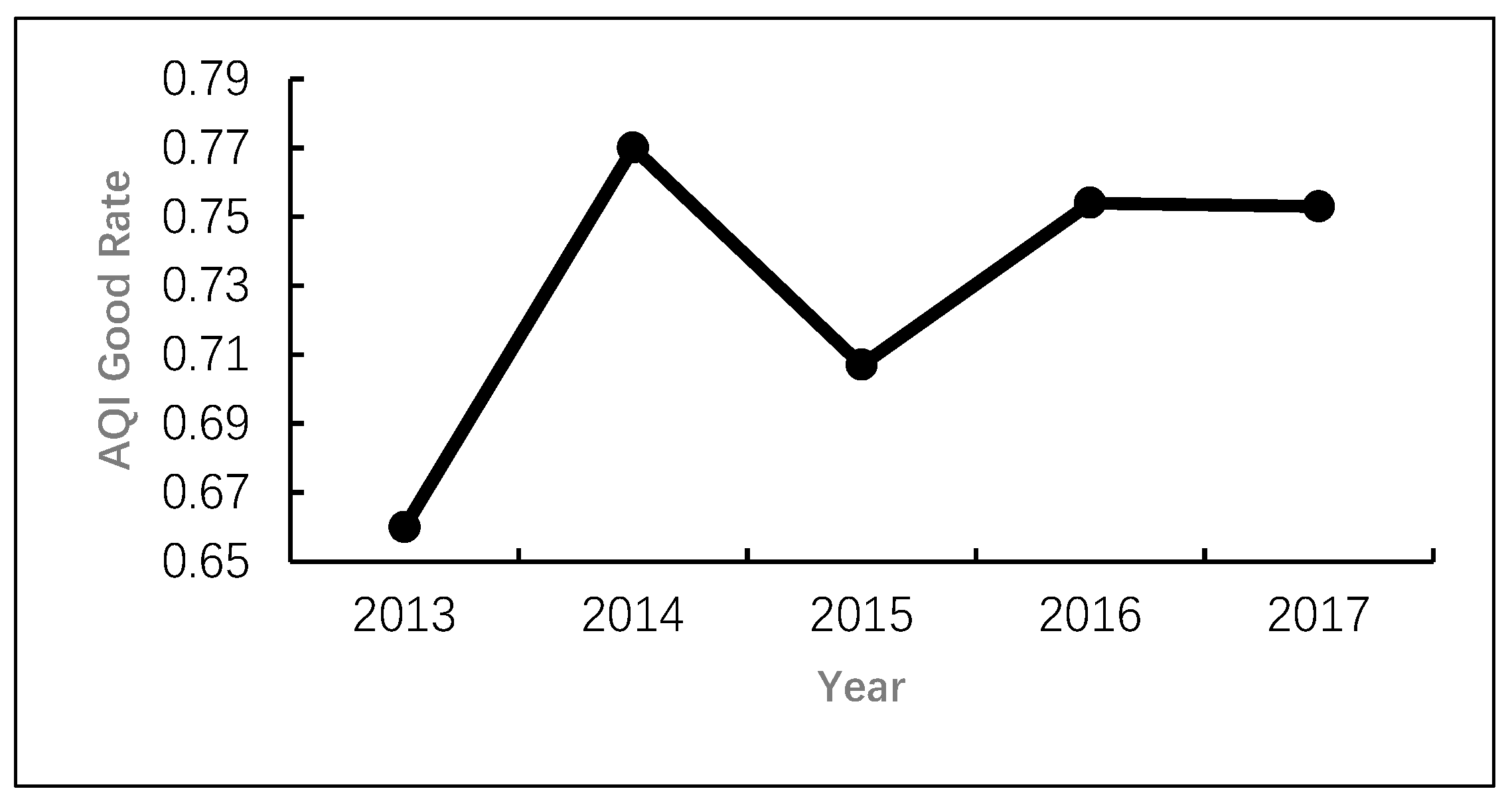
Figure 1 below shows the good rate of overall air quality (the ratio of air quality rated as Level I or II in Table 1) in Shanghai from 2013–2017 [23,37,38,39,40]. It can be seen from the figure that since 2013, Shanghai’s air quality has shown an improvement trend, despite a slight decline in 2015, which was mainly due to the fine particle pollution (PM_2.5) during autumn and winter, and ozone (O₃) pollution during summer.

2.3. Overview of Shanghai Climate

The climate of Shanghai is a typical subtropical maritime monsoon climate, mild and humid, with four distinct seasons. The spring in Shanghai is warm but often has sudden cold currents. The summer is hot with frequent heavy rains. The autumn is cool with dry weather. The winter is cold and accompanies fog and haze weather.

The Shanghai Meteorological Department began to accelerate the construction of automatic weather stations in 2002. Up to now, there are more than 200 automatic weather stations that have been built and used effectively [41]. The main observations indices of those stations include temperature, rainfall, air pressure, wind, visibility and dew point, etc. This paper selects 67 automatic stations with temperature observation records starting from 1 January 2006 and analyzes the climate data during the study period [42]. We found that Shanghai’s climate has the following distinct features:

(1) The climate in Shanghai is with a monthly average relative humidity of over 75%, and the annual precipitation is 1100 millimeters, which helps to relieve air pollution to some extent. So, Shanghai is a city with stable humidity. This will not cause the time difference of its PM_2.5.

(2) The average annual temperature is 16.7 °C. The average highest temperature in July and August is 28 °C and the extreme temperature in summer is 40.2 °C. The average lowest temperature in January is 4 °C, and the extreme temperature in winter is −12.1 °C [23].

(3) The northeast wind and the northwest wind are the dominant winds in winter, while the southeast wind and the southwest wind are the dominant winds in the summer. Because the east side of Shanghai is facing the sea, the easterly wind brings the clean air from the sea, while the westerly wind facilitates the spread of air pollutants from neighboring regions to Shanghai [43,44]. Shanghai is a city with many winds all year round. The average wind speed is relatively stable. At the same time, Shanghai is located in the plain, and there will be no conduction effect of pollutants due to wind direction problems.

2.4. Three Air Quality Assessment Methods

2.4.1. Comprehensive Pollution Index Method

In terms of the Comprehensive Pollution Index Method, the first step is to analyze the pollution load of the main air pollutants. The formula of the pollution load coefficient is as follows:

$$f_i=\frac{P_i}{P},P_i=\frac{C_i}{S_i},P={\displaystyle \sum }_{i=1}^k{P}_i$$

(3)

where:

• $C_i$ is the annual average concentration of the ith pollutant in the atmosphere;
• $S_i$ is the evaluation criteria of the ith pollutant in the atmosphere;
• $P_i$ is the sub-index of the ith pollutant;
• $f_i$ is the pollution load coefficient of the ith pollutant.

Then calculate the Comprehensive Pollution Index I according to Equation (2):

$$I=\sqrt{max\left(\frac{c_1}{s_1},\frac{c_2}{s_2},\dots ,\frac{c_k}{s_k}\right)}\frac{1}{k{{\displaystyle \sum }}_{i=1}^k\frac{c_i}{s_i}}$$

(4)

where:

• $c_k$ is the observed concentration value of a pollutant;
• $s_k$ is the corresponding evaluation criteria in Level II national air quality standard for the pollutant;
• I is the Comprehensive Pollution Index.

China issued the new Ambient Air Quality Standards (GB3095-2012) in 2012, which reclassified the atmospheric functional zones from the original three categories into two categories. Nature reserves, tourist attractions and other areas that require special protection belong to the first category, referred to as the Category I Zone, which applies to the Level I concentration limit. Commercial areas, industrial parks, and rural areas belong to the second category, referred to as the Category II Zone, which applies to the Level II concentration limit [27]. See

Table 2. Basic air pollutants assessment standards.

Pollutant	Average Value	Concentration Threshold		Unit of Measurement
		Level I	Level II
Sulfur Dioxide (SO2)	Annual Average	20	60	μg/m3
	24-h Average	50	150
	Hourly Average	150	500
Nitrogen Dioxide (NO2)	Annual Average	40	40	μg/m3
	24-h Average	80	80
	Hourly Average	200	200
Particulate Matter (PM10)	Annual Average	40	70	μg/m3
	24-h Average	50	150
Particulate Matter (PM2.5)	Annual Average	15	35	μg/m3
	24-h Average	35	75
Ozone (O3)	24-h Average	100	160	μg/m3
	Hourly Average	160	200
Carbonic Oxide (CO)	24-h Average	4	4	mg/m3
	Hourly Average	10	10

for the concentration limits of different functional zones.

The air quality can be evaluated by comparing the calculated Comprehensive Pollution Index I with the thresholds in the Air Quality Index scale.

Table 3. Air pollution grading system.

Air Quality Level	Clean	Mild Pollution	Moderate Pollution	Heavy Pollution	Severe Pollution
I	<0.6	0.6–1	1–1.9	1.9–2.8	>2.8
Pollution Level	Safe	Standard	Alert	Warning	Emergency

below has provided the Air Pollution Grading System.

The Comprehensive Pollution Index Method determines the air quality level based on the calculated pollution index value, and considers the average level of various pollutants and the damage level of a single pollutant in the calculation, which is simple and easy to conduct. However, the main disadvantage of this method is that when the value of the pollution index is exactly at the threshold between two air quality levels, it would be arbitrary to determine the air quality only based on one cut-off value and this would diminish the credibility of the evaluation result. Meanwhile, the calculation result depends on the ratio of the observed highest pollutant concentration value to the corresponding standard value, which would result in a higher Comprehensive Pollution Index if the observed value of a certain pollutant is relatively higher [45,46].

2.4.2. The Improved Grey Relational Degree Method

Let the reference sequence be $\left\{X_{i\left(k\right)}\right\}$. Compare the two sequences of $\left\{X_{j\left(k\right)}\right\}$ and $\left\{X_{i\left(k\right)}\right\}=\left\{X_{i\left(1\right)}, X_{i\left(2\right)},\dots X_{i\left(n\right)}\right\}, K=1,2,\dots n$. The correlation coefficient (${\xi }_{ij\left(k\right)}$) of $\left\{X_{i\left(k\right)}\right\}$ and $\left\{X_{j\left(k\right)}\right\}$ at point K (reflecting the correlation of the comparison sequence and the reference sequence at a certain point) can be defined by:

$${\xi }_{ij\left(k\right)}=\frac{\begin{array}{c}min\\ j\end{array}\begin{array}{c}min\\ k\end{array}{\Delta }_{ij\left(k\right)}+\rho \begin{array}{c}max\\ j\end{array}\begin{array}{c}max\\ k\end{array}{\Delta }_{ij\left(k\right)}}{{\Delta }_{ij\left(k\right)}+\rho \begin{array}{c}max\\ j\end{array}\begin{array}{c}max\\ k\end{array}{\Delta }_{ij\left(k\right)}}$$

(5)

where:

• ${\Delta }_{ij\left(k\right)}=\left|X_{i\left(k\right)}-X_{j\left(k\right)}\right|$ is the difference in the absolute value of $\left\{X_{i\left(k\right)}\right\}$ and $\left\{X_{j\left(k\right)}\right\}$ at point K;
• $\begin{array}{c}min\\ j\end{array}\begin{array}{c}min\\ k\end{array}{\Delta }_{ij\left(k\right)}$ is the minimum differnce between two levels;
• $\begin{array}{c}max\\ j\end{array}\begin{array}{c}max\\ k\end{array}{\Delta }_{ij\left(k\right)}$ is the maximum difference between two levels;
• $\rho$ is the distinguishing coefficient, which takes a value between 0 and 1. After comparing the $\rho$ values in the related literature [47,48], we set $\rho =0.5$ to avoid the influence of the extreme values on the calculation results.

Integrate the correlation coefficients at different points $\left(K=1,2\dots n\right)$ to obtain the overall correlation of the comparison sequence $\left\{X_{j\left(k\right)}\right\}$ and the reference sequence $\left\{X_{i\left(k\right)}\right\}$, as shown in the following equation:

$${\gamma }_{i,j}=\frac{1}{n}{\displaystyle \sum }_{k=1}^n{\xi }_{ij\left(k\right)}$$

(6)

If $\left\{X_{1\left(k\right)}\right\},\left\{X_{2\left(k\right)}\right\},\dots ,\left\{X_{j\left(k\right)}\right\}$ are N known comparison sequences, and $\left\{X_{i\left(k\right)}\right\}$ is a known reference series, there would be:

$${\gamma }_{i,s}{}^{*}=max\left\{{\gamma }_{i,j}\right\},1\le j\le n$$

(7)

At this time, the reference sequence $\left\{X_{i\left(k\right)}\right\}$ would have the best correlation with the comparison sequence $\left\{X_{j\left(k\right)}\right\}$.

Obviously, if $\left\{X_{i\left(k\right)}\right\}$ represents the sequence made up by the observed mass concentration values of different pollutants, $\left\{X_{j\left(k\right)}\right\}$ represents the sequence made up by the evaluation standards of a certain level of different pollutants. Because of the good correlation between $\left\{X_{i\left(k\right)}\right\}$ and $\left\{X_{j\left(k\right)}\right\}$, it is most appropriate to evaluate the air quality of Sample Point i as the corresponding Level S.

Furthermore, normalize the data. Let $S\left(k,j\right)=\raisebox{1ex}{$S_{Kj}$}\!\left/ \!\raisebox{-1ex}{$S_{Ij}$}\right.$ be the equal-standard grading standard, and $I\left(i,j\right)=\raisebox{1ex}{$C_{ij}$}\!\left/ \!\raisebox{-1ex}{$S_{Ij}$}\right.$ be the Air Pollution Index to be evaluated. The weight of the pollutant $w\left(i,j\right)$ can be written as follows:

$$w\left(i,j\right)=\frac{log100I\left(i,j\right)}{{{\displaystyle \sum }}_{i=1}^{k}log100I\left(i,j\right)}$$

(8)

where:

• $S_{Kj}$ is the Graded Index of the jth pollution indicator on Level K;
• $S_{Ij}$ is the Graded Index of the jth pollution indicator on Level I;
• $C_{ij}$ is the observed value of the jth pollution indicator in the ith monitoring point.

Based on this, the correlation between the quality of air samples to be evaluated and the standard air quality of different levels can be calculated by:

$$G\left(i,k\right)={\displaystyle \sum }_{i=1}^{k}W\left(i,j\right).{\gamma }_{i,s}{}^{*}$$

(9)

The traditional Grey Relational Degree Method is relatively simple in calculation. However, when the pollution factors are significantly different, the average value with equal weights would understate the pollution factor with high concentration while overstate the pollution factor with low concentration, which would differ from the actual pollution condition [49,50,51]. The improved method above determines different air quality levels based on the observed concentration of different pollution factors, and calculates the weights and correlation coefficients of each pollution factor accordingly. When evaluating the air quality, the Improved Grey Relational Degree Method not only enhances the weights of the pollution factors with high concentration, but also takes into account the combined effects of different pollution factors on air quality, so that basically no information is lost during the evaluation process. It also comprehensively considers the effects of different pollutant weights and the interactions between different pollutants, thus improving the accuracy of the evaluation result.

2.4.3. Euclid Approach Degree Method

First, determine the characteristic value $\lambda \left(K,j\right)$ of the pollution level, as shown in the following equation:

$$\lambda \left(K,j\right)=\{\begin{array}{c}\raisebox{1ex}{$S_{Kj}$}\!\left/ \!\raisebox{-1ex}{$2$}\right.,K=1\\ \raisebox{1ex}{$\left[S_{Kj}+S_{K-1j}\right]$}\!\left/ \!\raisebox{-1ex}{$2$}\right.,K=2\end{array}$$

(10)

where $S_{Kj}$ represents the grading index of the jth pollutant of Level K.

Then determine the index weight $w\left(i,j\right)$ of different pollutants:

$$w\left(i,j\right)=\frac{({\lambda }_{Kj}+x_{ij})/\overline{{\lambda }_J}}{{{\displaystyle \sum }}_{i=1}^n({\lambda }_{Kj}+x_{ij})/\overline{{\lambda }_J}}$$

(11)

where:

• $x_{ij}$ represents the observed concentration value of the jth pollution indicator at the ith monitoring point;
• $\overline{{\lambda }_J}$ represents the the mean value of the characteristic values of different levels of the jth pollution indicator;
• ${\lambda }_{kj}$ represents the characteristic value of Level II of the jth pollution indicator.

Normalize the observed result by:

$$x\left(i,j\right)=x_{ij}/{\lambda }_{kj}$$

Calculate the Proximity Degree $\eta (i,j)$ of the air sample to be evaluated:

$$\eta \left(i,j\right)=\sqrt{{\displaystyle \sum }_{i=1}^{n}W\left(i,j\right){\left[x\left(i,j\right)-\lambda \left(i,j\right)\right]}^2}$$

Then, determine the respective air quality level of each monitoring point based on the principle of minimum proximity degree.

For evaluation purpose, the Euclid Approach Degree Method needs to establish two membership functions of the observed value and the standard level. All valid data observed have been taken into consideration in the modeling and calculation process. Therefore, there won’t be any information loss during the evaluation process and the actual condition of the environment could be comprehensively reflected [52,53,54].

3. Results

The study period of this paper is from 1 November 2017 to 31 October 2018. The air pollutants as the study object include SO₂, NO₂, PM₁₀, PM_2.5, O₃ and CO. The seasons are determined based on the months: Spring (March, April, May), summer (June, July, August), autumn (September, October, November), and winter (December, January, February). See

Table 4. Average Concentration of Main Air Pollutants by Season ($\mathsf{\mu }\mathrm{g}/{\mathrm{m}}^3$).

	Pollutant	PM2.5	PM10	SO2	NO2	O3	CO
Season
Winter		52.00	66.67	14.33	58.00	83	0.82
Spring		42.33	62.67	12.00	44.33	97	0.76
Summer		24.33	36.67	8.00	25.33	112	0.68
Autumn		31.67	52.67	9.67	46.00	103	0.53

for the average concentration levels of various air pollutants in different seasons.

The Air Pollution Grading Indexes of different seasons obtained through the Comprehensive Pollution Grading Method are shown in

Table 5. Comprehensive Pollution Grading Index by Season.

Season	Winter	Spring	Summer	Autumn
Comprehensive Pollution Index	1.24	1.02	0.59	0.92

.

It can be seen from Table 5 that from 1 November 2017 to 31 October 2018, the average air quality in Shanghai during winter (December, January, February) was heavy pollution; the average air quality during spring (March, April, May) was moderate pollution; the average air quality during summer (June, July, August) was clean; while the average air quality during autumn (September, October, November) was mild pollution. The results above indicate that the air quality of Shanghai was still not ideal and further pollution control measures are needed.

Table 6. Air Pollution Grading Index by season obtained by the improved grey relational degree method and the Euclid approach degree method.

	Method	Improved Grey Relational Degree Method	Euclid Approach Degree Method
Season
Winter		II	II
Spring		II	II
Summer		I	I
Autumn		I	II

has shown the Air Pollution Grading Index by season obtained through the Improved Grey Relational Degree Method and the Euclid Approach Degree Method introduced in Part 2.4 (please refer to Appendix A for the MATLAB algorithm—MATLAB 2017b, MathWorks, Natick, USA).

It can be seen that the evaluation results obtained through the Improved Grey Relational Degree Method and the Euclid Approach Degree Method are consistent except for autumn. The air quality in winter has met the Level II national air quality standard stipulated in GB3095-2012; the air quality in spring has also met the Level II standard; while the air quality in summer has reached the Level I national air quality standard.

It can be seen from the calculation results obtained by the three evaluation methods above that there is some concern in the air quality of Shanghai, especially during winters when the air pollution is most severe.

4. Discussion

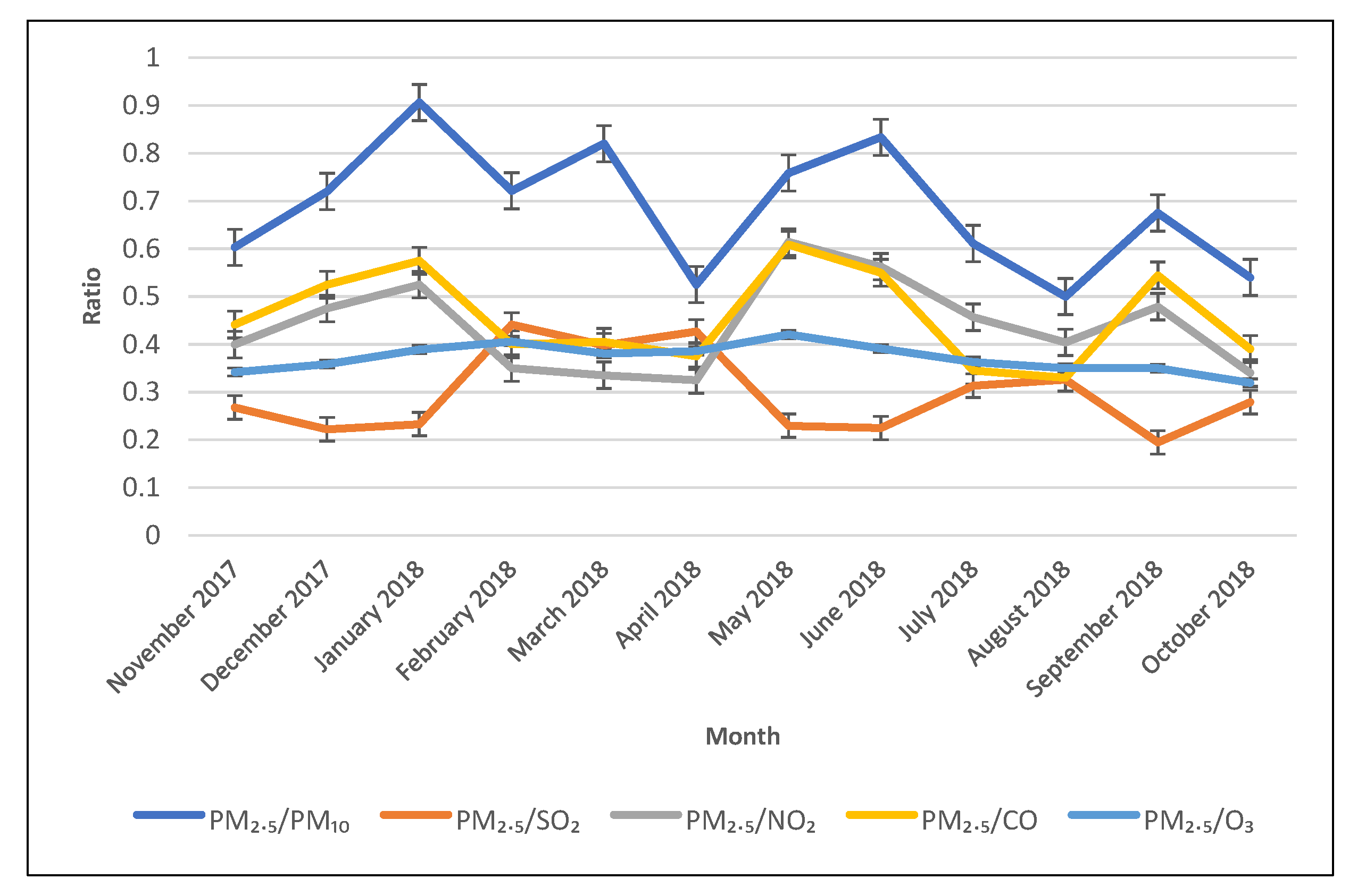
Based on the above calculation results, this paper further analyzes the fine particle pollution of Shanghai during the study period. The particulate pollutants in the atmosphere can be categorized into total suspended particulates (TSP), PM₁₀, and PM_2.5 based on the particle size [55,56,57]. TSP generally refers to the particulate matters floating in the air with a particle size of less than 100 $\mathsf{\mu }\mathrm{m}$, including solid particles and liquid particles [58,59]. PM₁₀ refers to particulate matters with a particle size of 10 $\mathsf{\mu }\mathrm{m}$ or less. Most PM₁₀ could reach the throat or even further in the respiratory tract [60,61]. PM_2.5 refers to particulate matters with a particle size of below 2.5 $\mathsf{\mu }\mathrm{m}$. Most PM_2.5 can settle in the respiratory tract, and a small number of PM_2.5 could even reach the pulmonary alveoli which are very difficult to get rid of and extremely harmful to the human body [62,63,64]. In recent research, PM_2.5 and PM₁₀ have been the focus of air pollution control in China [65,66,67,68]. According to studies at home and abroad, there exist certain correlations between PM₁₀ and PM_2.5 [69,70,71,72]. In order to fully understand the relationship between PM_2.5 and other major pollutants in Shanghai, we have calculated the ratio of PM_2.5/PM₁₀, PM_2.5/SO₂, PM_2.5/NO₂, PM_2.5/CO, and PM_2.5/O₃, according to the 2017 Shanghai Environmental Bulletin [26] and the Shanghai Air Quality Monthly Report from January–October 2018 [73]. The results showed that the variation range of PM_2.5/PM₁₀ was [0.4–0.7], while the ratio of PM_2.5/SO₂, PM_2.5/NO₂, PM_2.5/CO, and PM_2.5/O₃ was low (see Figure 2).

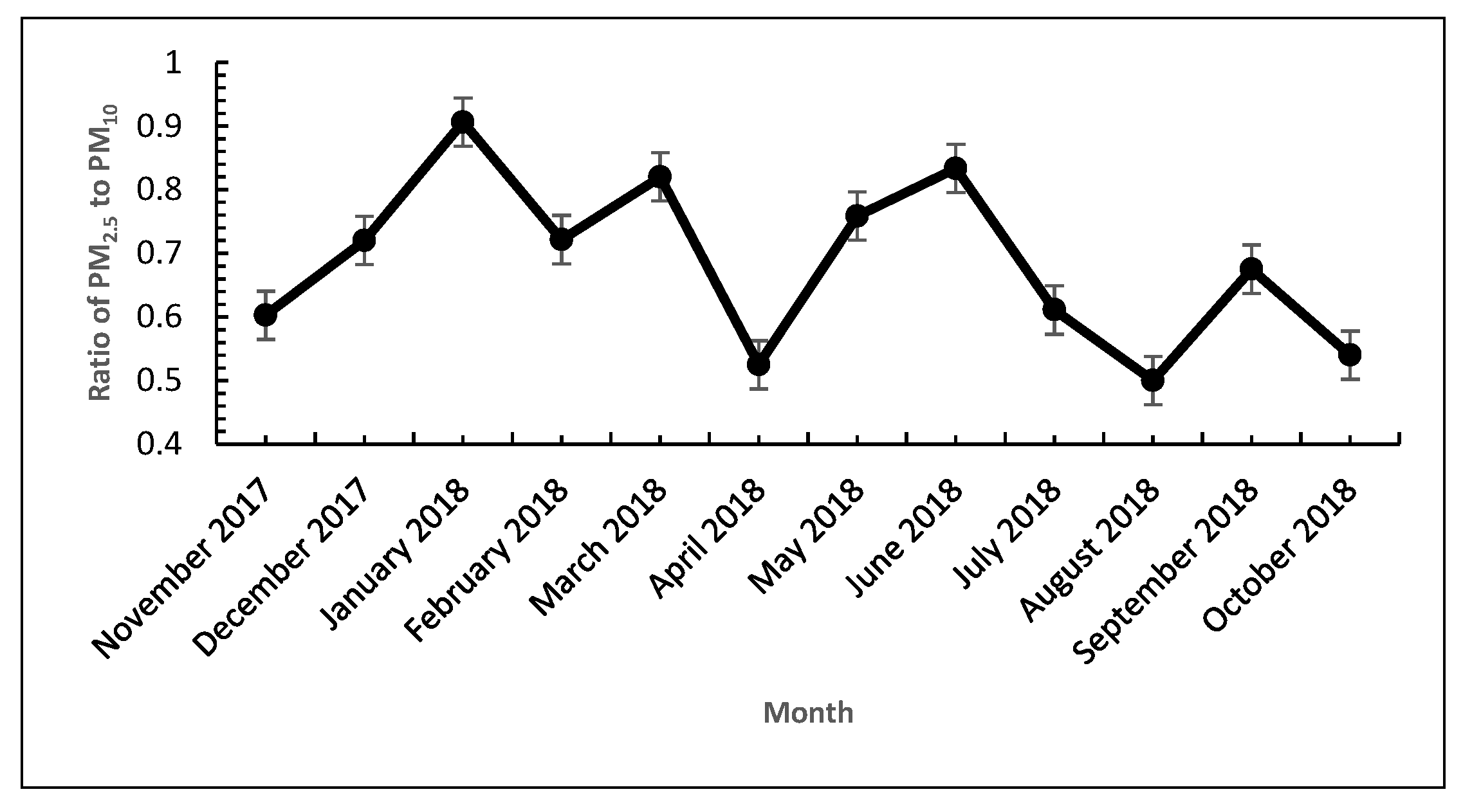
Hence, we will focus on the correlation between PM_2.5 and PM₁₀ concentration in Shanghai. The ratio of PM_2.5/PM₁₀ in Shanghai ranged from 0.50–0.91 during the study period [23,73]. The monthly ratios are shown in Figure 3 below, which was highest in January and lowest in August. Overall speaking, the ratios were volatile, with an average value of 0.68. Among the 90 pollution days in 2017 as published in 2017 Shanghai Environmental Bulletin, there are 25.6% of the days in which fine particles (PM_2.5) was the primary air pollutant [23].

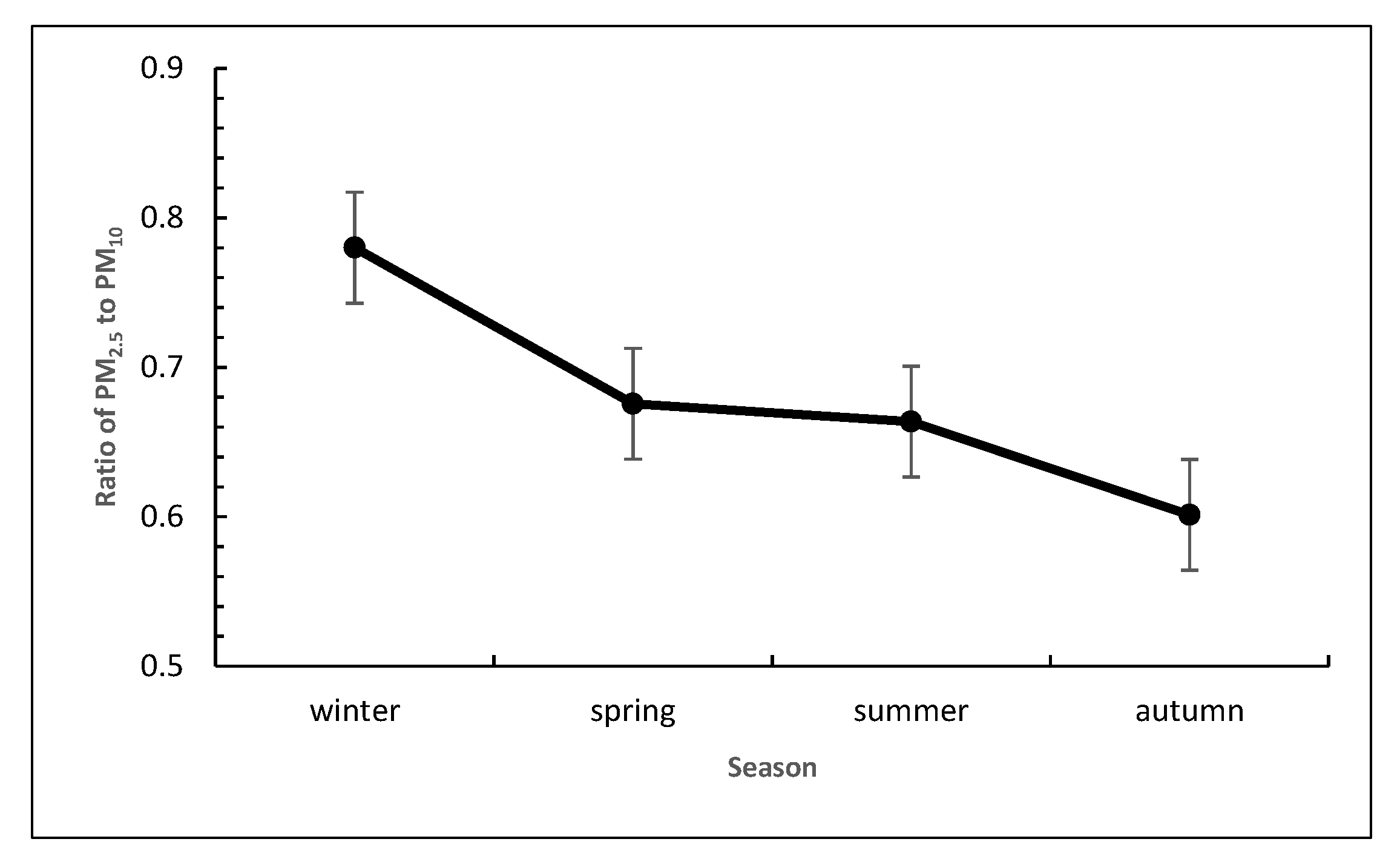
It can be seen from the seasonal change of the PM_2.5/PM₁₀ ratio in Figure 4 that the seasonal trend of this ratio is: winter > spring > summer > autumn. Meanwhile, this ratio in winter is 1.3 times of that in summer. According to the relevant literature, we found that it is due to the increased energy consumption in winter heating, less rainfall and more fog weathers in winters, which do not facilitate the movement of fine particles and results in less sedimentation. In springs, the increased wind frequency and air flow, especially the northwest wind would bring coarse particulate pollution to Shanghai. In summers, the high temperature and rising hot air do not facilitate the sedimentation of fine particles. In autumns, the cool weather and air flow help to spread and subside fine particles, and therefore the degree of fine particle pollution is lower [74,75,76,77,78].

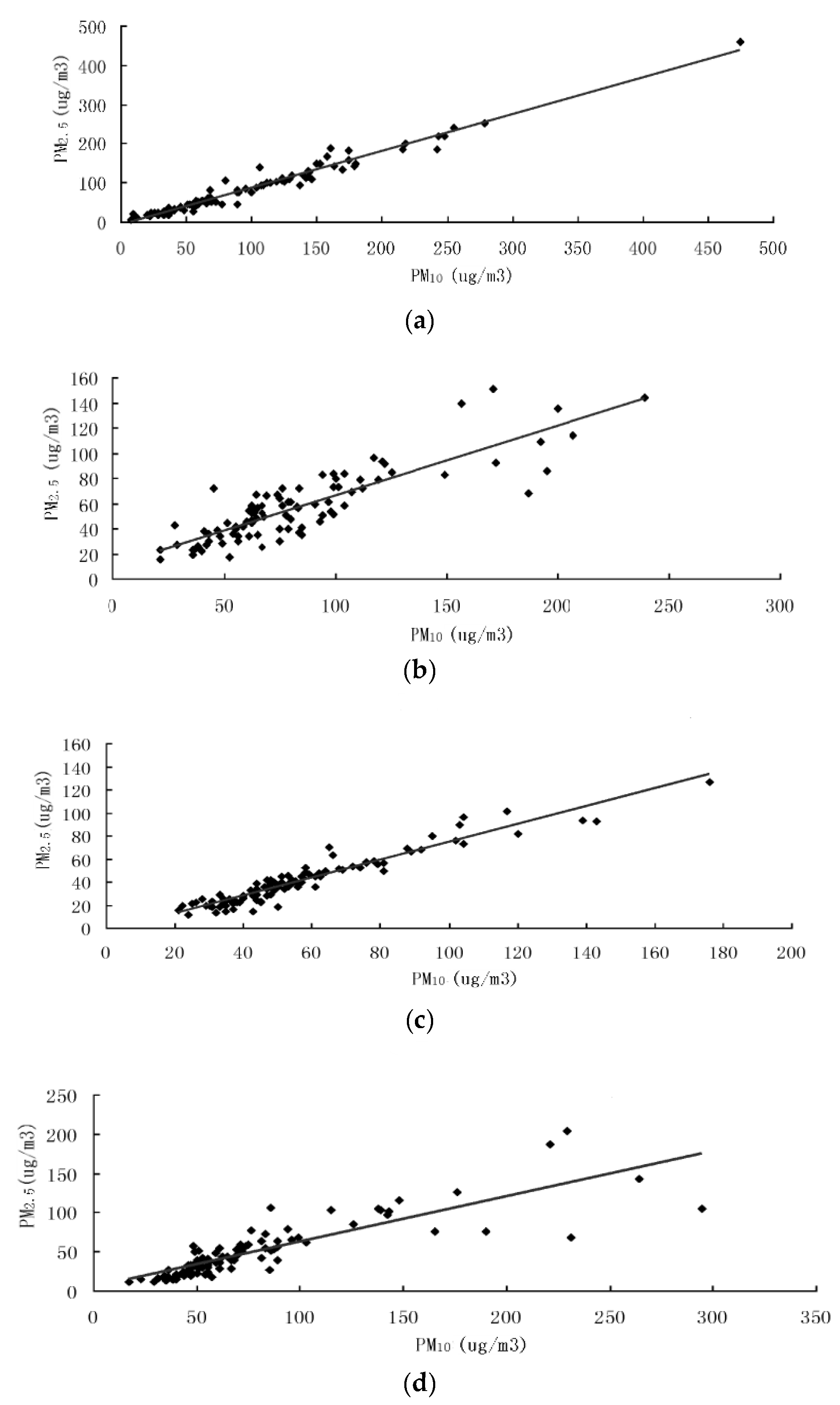
Through the quarterly linear regression analysis of PM_2.5 and PM₁₀ in Shanghai from 1 November 2017 to 31 October 2018, this paper has found a significant linear relationship between PM_2.5 and PM₁₀.

As shown in Figure 5a, although the linear correlation between PM_2.5 and PM₁₀ varies from season to season, there is still a strong correlation between PM_2.5 and PM₁₀ concentrations, which is the strongest during winters and summers. In winter, the correlation coefficient reached $R^2=0.9655$, while in summer, the correlation coefficient $R^2=0.9112$. The corresponding regression equations are $y=0.9333x-5.2223$ and $y=0.7734x-2.614$, respectively. Taking winter as an example, the t-test on the three-month data of winter provided a confidence interval of [53.4543, 68.4943] with 95% confidence, and a significance probability of 0, which is less than 0.05. Therefore, we can say there is a significant linear relationship between PM_2.5 and PM₁₀ concentration in winter. In spring and autumn, there is also a linear relationship between PM_2.5 and PM₁₀ concentration, but the correlation coefficient is smaller. The regression equation in spring is $y=0.5524x-11.206$, with a correlation coefficient of $R^2=0.7379$; while the regression equation in autumn is $y=0.5731x+5.597$, with a correlation coefficient of $R^2=0.7282$.

The regression fitting results above show that there is a significant linear relationship between PM_2.5 and PM₁₀ concentration in winters and summers, while their linear correlation is less significant during spring and autumn, which is mainly due to temperature reasons. The cold weather in winters and hot weather in summers of Shanghai do not facilitate the spread of particle pollutants. The particles tend to float in the air, showing a significant linear correlation. On the other hand, in springs and autumns, the temperature is moderate with frequent and strong monsoon which helps to increase air flow and facilitate the diffusion and sedimentation of particle pollutants. Fine particles and coarse particles respond differently to these climate factors. Therefore, the linear correlation between the mass concentration of particulate matters PM_2.5 and PM₁₀ is less significant in springs and autumns.

Although air quality has shown improvement in the past decade, there are numerous challenges in the coming years. With the construction of the Yangtze River Delta urban agglomeration and the Yangtze River Economic Belt during the 13th Five-Year Plan period, there will be strong economic growth as well as a continuous increase in air pollutant emissions in neighboring cities and other provinces and cities at the upper and middle region of the Yangtze River. If we cannot establish an effective and coordinated regional air pollution prevention and control mechanism, it would greatly affect Shanghai’s air quality. Moreover, since the parameters we used are derived from official data from Shanghai [21,23,36,37,38,39,40,73], and the aforementioned research methods have been widely recognized in the academic world, the research design of this paper has exportability under the premise of using other reliable data sources.

5. Conclusions

This paper has evaluated the quarterly air quality of Shanghai by using the Comprehensive Pollution Index Method, the Improved Grey Relational Degree Method, and the Euclid Approach Degree Method and based on the technical norms of China’s current AQI and analysis of Shanghai’s overall climate. By analysis on the air pollutants (SO₂, NO₂, PM₁₀ and PM_2.5) in Shanghai from 1 November 2017 to 31 October 2018, this paper has reached the following conclusions:

(1) The air quality of Shanghai has moderate pollution in winters and springs, clean in summers, and mild pollution in autumns. The evaluation results obtained by the Improved Grey Relational Degree Method and the Euclid Approach Degree Method are basically consistent. The air quality in winter has met the Level II national air quality standard in GB3095-2012; the air quality in spring has also met the Level II standard; while the air quality in summer has reached the Level I national air quality standard. These results are consistent between the Improved Grey Relational Degree Method and the Euclid Approach Degree Method. However, in autumn, the air quality evaluation result according to the Improved Grey Relational Degree Method is Level I, while the evaluation result according to the Euclid Approach Degree Method is Level II. Therefore, there exist some concern in the air quality of Shanghai, especially during winters when the air pollution is most severe.

(2) The air pollutants in Shanghai have shown a seasonal pattern of high concentration in winters and low concentration in summers; meanwhile, the pollutant concentration is higher in the first half of the year than in the second half. This is because the first half of the year is the peak period of industrial energy consumption, and both industrial and residential heating needs in winter would inevitably cause increase in energy consumption such as the coal [79], which would undoubtedly increase the concentration of air pollutants.

(3) By analyzing the particle pollutants of PM_2.5 and PM₁₀, this paper has found that the linear correlation between the two varies with the seasons, which is most significant during winters and summers.

References

- Zhang, D.; Liu, J.; Li, B. Tackling Air Pollution in China—What do We Learn from the Great Smog of 1950s in LONDON. Sustainability 2014, 6, 5322–5338. [Google Scholar] [CrossRef]
- Yang, W.; Li, L. Energy efficiency, ownership structure, and sustainable development: Evidence from China. Sustainability 2017, 9, 912. [Google Scholar] [CrossRef]
- Yang, Y.; Yang, W. Does Whistleblowing Work for Air Pollution Control in China? A Study Based on Three-party Evolutionary Game Model under Incomplete Information. Sustainability 2019, 11, 324. [Google Scholar] [CrossRef]
- Yuan, G.; Yang, W. Evaluating China’s Air Pollution Control Policy with Extended AQI Indicator System: Example of the Beijing-Tianjin-Hebei Region. Sustainability 2019, 11, 939. [Google Scholar] [CrossRef]
- Li, H.; Tan, X.; Guo, J.; Zhu, K.; Huang, C. Study on an Implementation Scheme of Synergistic Emission Reduction of CO2 and Air Pollutants in China’s Steel Industry. Sustainability 2019, 11, 352. [Google Scholar] [CrossRef]
- Bloss, W. Measurement of Air Pollutants. In Reference Module in Earth Systems and Environmental Sciences; Elsevier: Amsterdam, The Netherlands, 2018; ISBN 978-0-12-409548-9. [Google Scholar]
- Park, J.H.; Lee, S.H.; Yun, S.J.; Ryu, S.; Choi, S.W.; Kim, H.J.; Kang, T.K.; Oh, S.C.; Cho, S.J. Air pollutants and atmospheric pressure increased risk of ED visit for spontaneous pneumothorax. Am. J. Emerg. Med. 2018, 36, 2249–2253. [Google Scholar] [CrossRef] [PubMed]
- Filonchyk, M.; Yan, H.; Li, X. Temporal and spatial variation of particulate matter and its correlation with other criteria of air pollutants in Lanzhou, China, in spring-summer periods. Atmos. Pollut. Res. 2018, 9, 1100–1110. [Google Scholar] [CrossRef]
- Dirgawati, M.; Heyworth, J.S.; Wheeler, A.J.; McCaul, K.A.; Blake, D.; Boeyen, J.; Cope, M.; Yeap, B.B.; Nieuwenhuijsen, M.; Brunekreef, B.; et al. Development of Land Use Regression models for particulate matter and associated components in a low air pollutant concentration airshed. Atmos. Environ. 2016, 144, 69–78. [Google Scholar] [CrossRef]
- Son, Y.; Osornio-Vargas, Á.R.; O’Neill, M.S.; Hystad, P.; Texcalac-Sangrador, J.L.; Ohman-Strickland, P.; Meng, Q.; Schwander, S. Land use regression models to assess air pollution exposure in Mexico City using finer spatial and temporal input parameters. Sci. Total Environ. 2018, 639, 40–48. [Google Scholar] [CrossRef]
- Tao, H.; Xing, J.; Zhou, H.; Chang, X.; Li, G.; Chen, L.; Li, J. Impacts of land use and land cover change on regional meteorology and air quality over the Beijing-Tianjin-Hebei region, China. Atmos. Environ. 2018, 189, 9–21. [Google Scholar] [CrossRef]
- Pérez, J.F.; Sabatino, S.; Galia, A.; Rodrigo, M.A.; Llanos, J.; Sáez, C.; Scialdone, O. Effect of air pressure on the electro-Fenton process at carbon felt electrodes. Electrochim. Acta 2018, 273, 447–453. [Google Scholar] [CrossRef]
- Kalisa, E.; Fadlallah, S.; Amani, M.; Nahayo, L.; Habiyaremye, G. Temperature and air pollution relationship during heatwaves in Birmingham, UK. Sustain. Cities Soc. 2018, 43, 111–120. [Google Scholar] [CrossRef]
- Yu, Y.; Kwok, K.C.S.; Liu, X.P.; Zhang, Y. Air pollutant dispersion around high-rise buildings under different angles of wind incidence. J. Wind Eng. Ind. Aerodyn. 2017, 167, 51–61. [Google Scholar] [CrossRef]
- Yang, W.; Li, L. Efficiency evaluation of industrial waste gas control in China: A study based on data envelopment analysis (DEA) model. J. Clean. Prod. 2018, 179, 1–11. [Google Scholar] [CrossRef]
- Cheng, M.; Zhi, G.; Tang, W.; Liu, S.; Dang, H.; Guo, Z.; Du, J.; Du, X.; Zhang, W.; Zhang, Y.; et al. Air pollutant emission from the underestimated households’ coal consumption source in China. Sci. Total Environ. 2017, 580, 641–650. [Google Scholar] [PubMed]
- Cai, P.; Nie, W.; Chen, D.; Yang, S.; Liu, Z. Effect of air flowrate on pollutant dispersion pattern of coal dust particles at fully mechanized mining face based on numerical simulation. Fuel 2019, 239, 623–635. [Google Scholar] [CrossRef]
- Liu, B.; Wu, S.; Shen, L.; Zhao, T.; Wei, Y.; Tang, X.; Long, C.; Zhou, Y.; He, D.; Lin, T.; et al. Spermatogenesis dysfunction induced by PM2.5 from automobile exhaust via the ROS-mediated MAPK signaling pathway. Ecotoxicol. Environ. Saf. 2019, 167, 161–168. [Google Scholar] [CrossRef]
- Yang, W.; Li, L. Analysis of Total Factor Efficiency of Water Resource and Energy in China: A Study Based on DEA-SBM Model. Sustainability 2017, 9, 1316. [Google Scholar]
- Li, L.; Yang, W. Total Factor Efficiency Study on China’s Industrial Coal Input and Wastewater Control with Dual Target Variables. Sustainability 2018, 10, 2121. [Google Scholar] [CrossRef]
- Shanghai Municipal Statistics Bureau. Shanghai Statistical Yearbook 2017; China Statistics Press: Shanghai, China, 2018.
- National Bureau of Statistics of the People’s Republic of China. China Statistical Yearbook 2017; China Statistics Press: Beijing, China, 2018.
- Shanghai Municipal Environmental Protection Bureau. 2017 Shanghai Environmental Bulletin; Shanghai Municipal Environmental Protection Bureau: Shanghai, China, 2018.
- Ministry of Environmental Protection of the People’s Republic of China. Ambient Air Quality Standards: GB3095-2012; China Environmental Science Press: Beijing, China, 2012.
- Ministry of Environmental Protection of the People’s Republic of China. Technical Regulation on Ambient Air Quality Index (on Trial): HJ 633-2012; China Environmental Science Press: Beijing, China, 2012.
- Li, X.; Gao, Z.; Li, Y.; Gao, C.Y.; Ren, J.; Zhang, X. Meteorological conditions for severe foggy haze episodes over north China in 2016–2017 winter. Atmos. Environ. 2019, 199, 284–298. [Google Scholar] [CrossRef]
- Golly, B.; Waked, A.; Weber, S.; Samake, A.; Jacob, V.; Conil, S.; Rangognio, J.; Chrétien, E.; Vagnot, M.P.; Robic, P.Y.; et al. Organic markers and OC source apportionment for seasonal variations of PM2.5 at 5 rural sites in France. Atmos. Environ. 2019, 198, 142–157. [Google Scholar] [CrossRef]
- Ryu, J.; Kim, J.J.; Byeon, H.; Go, T.; Lee, S.J. Removal of fine particulate matter (PM2.5) via atmospheric humidity caused by evapotranspiration. Environ. Pollut. 2019, 245, 253–259. [Google Scholar] [CrossRef] [PubMed]
- United States Environmental Protection Agency. Air Emissions Inventories; United States Environmental Protection Agency: Washington, DC, USA, 2018.
- European Environment Agency. EMEP/EEA Air Pollutant Emission Inventory Guidebook 2016; European Environment Agency: Copenhagen, Denmark, 2016.
- Ohara, T.; Akimoto, H.; Kurokawa, J.I.; Horii, N.; Yamaji, K.; Yan, X.; Hayasaka, T. An Asian emission inventory of anthropogenic emission sources for the period 1980–2020. Atmos. Chem. Phys. 2007, 7, 4419–4444. [Google Scholar]
- Kim, J.-H.; Park, J.-M.; Lee, S.-B.; Pudasainee, D.; Seo, Y.-C. Anthropogenic mercury emission inventory with emission factors and total emission in Korea. Atmos. Environ. 2010, 44, 2714–2721. [Google Scholar] [CrossRef]
- Kim, N.K.; Kim, Y.P.; Morino, Y.; Kurokawa, J.; Ohara, T. Verification of NOx emission inventory over South Korea using sectoral activity data and satellite observation of NO2 vertical column densities. Atmos. Environ. 2013, 77, 496–508. [Google Scholar] [CrossRef]
- Kannari, A.; Streets, D.G.; Tonooka, Y.; Murano, K.; Baba, T. MICS-Asia II: An inter-comparison study of emission inventories for the Japan region. Atmos. Environ. 2008, 42, 3584–3591. [Google Scholar] [CrossRef]
- Li, Y.; Qian, X.; Zhang, L.; Dong, L. Exploring spatial explicit greenhouse gas inventories: Location-based accounting approach and implications in Japan. J. Clean. Prod. 2017, 167, 702–712. [Google Scholar] [CrossRef]
- Shanghai Municipal Environmental Protection Bureau. 2012 Shanghai Environmental Bulletin; Shanghai Municipal Environmental Protection Bureau: Shanghai, China, 2013.
- Shanghai Municipal Environmental Protection Bureau. 2013 Shanghai Environmental Bulletin; Shanghai Municipal Environmental Protection Bureau: Shanghai, China, 2014.
- Shanghai Municipal Environmental Protection Bureau. 2014 Shanghai Environmental Bulletin; Shanghai Municipal Environmental Protection Bureau: Shanghai, China, 2015.
- Shanghai Municipal Environmental Protection Bureau. 2015 Shanghai Environmental Bulletin; Shanghai Municipal Environmental Protection Bureau: Shanghai, China, 2016.
- Shanghai Municipal Environmental Protection Bureau. 2016 Shanghai Environmental Bulletin; Shanghai Municipal Environmental Protection Bureau: Shanghai, China, 2017.
- Shen, Z.; Liang, P.; He, J. Analysis on the climatic characteristics of the fine structure of the urban heat island in Shanghai. Trans. Atmos. Sci. 2017, 40, 369–378. [Google Scholar]
- Meteorological Data Center of China Meteorological Administration Observation Data of Shanghai Ground Meteorology. Available online: https://data.cma.cn/ (accessed on 17 March 2019).
- Guo, H.; Chen, M. Short-term effect of air pollution on asthma patient visits in Shanghai area and assessment of economic costs. Ecotoxicol. Environ. Saf. 2018, 161, 184–189. [Google Scholar] [CrossRef] [PubMed]
- Ji, X.; Meng, X.; Liu, C.; Chen, R.; Ge, Y.; Kan, L.; Fu, Q.; Li, W.; Tse, L.A.; Kan, H. Nitrogen dioxide air pollution and preterm birth in Shanghai, China. Environ. Res. 2019, 169, 79–85. [Google Scholar] [CrossRef] [PubMed]
- Xiaoyu, L.; Jun, Y.; Pengfei, S. Structure and Application of a New Comprehensive Environmental Pollution Index. Energy Procedia 2011, 5, 1049–1054. [Google Scholar] [CrossRef]
- Gąsiorek, M.; Kowalska, J.; Mazurek, R.; Pająk, M. Comprehensive assessment of heavy metal pollution in topsoil of historical urban park on an example of the Planty Park in Krakow (Poland). Chemosphere 2017, 179, 148–158. [Google Scholar] [CrossRef] [PubMed]
- Zhu, C.; Li, N. Study on Grey Clustering Model of Indoor Air Quality Indicators. Procedia Eng. 2017, 205, 2815–2822. [Google Scholar] [CrossRef]
- Yunlong, W.; Kai, L.; Guan, G.; Yanyun, Y.; Fei, L. Evaluation method for Green jack-up drilling platform design scheme based on improved grey correlation analysis. Appl. Ocean Res. 2019, 85, 119–127. [Google Scholar] [CrossRef]
- Yan, F.; Qiao, D.; Qian, B.; Ma, L.; Xing, X.; Zhang, Y.; Wang, X. Improvement of CCME WQI using grey relational method. J. Hydrol. 2016, 543, 316–323. [Google Scholar] [CrossRef]
- Sun, G.; Guan, X.; Yi, X.; Zhou, Z. Grey relational analysis between hesitant fuzzy sets with applications to pattern recognition. Expert Syst. Appl. 2018, 92, 521–532. [Google Scholar] [CrossRef]
- Li, X.; Wang, Z.; Zhang, L.; Zou, C.; Dorrell, D.D. State-of-health estimation for Li-ion batteries by combing the incremental capacity analysis method with grey relational analysis. J. Power Sources 2019, 410–411, 106–114. [Google Scholar] [CrossRef]
- Du, X.; Yang, Z.; Li, G.; Jia, Y.; Chen, C.; Gui, L. Remaining useful life assessment of machine tools based on AHP method and Euclid approach degree. In Proceedings of the International Conference on System Reliability and Science (ICSRS), Paris, France, 15–18 November 2016; pp. 46–52. [Google Scholar]
- Wang, S.; Zhang, T.; Cheng, L.; Li, J.; Tang, H.; Guo, M. Comprehensive performance of compound fabrics in terms of electromagnetic shielding and wearability based on the Euclid approach degree of fuzzy matter elements. J. Text. Inst. 2017, 108, 341–346. [Google Scholar]
- Niu, D.; Song, Z.; Wang, M.; Xiao, X. Improved TOPSIS method for power distribution network investment decision-making based on benefit evaluation indicator system. Int. J. Energy Sect. Manag. 2017, 11, 595–608. [Google Scholar]
- Gysel, N.; Welch, W.A.; Chen, C.-L.; Dixit, P.; Cocker, D.R.; Karavalakis, G. Particulate matter emissions and gaseous air toxic pollutants from commercial meat cooking operations. J. Environ. Sci. 2018, 65, 162–170. [Google Scholar] [CrossRef]
- Feng, Y.; Li, Y.; Cui, L. Critical review of condensable particulate matter. Fuel 2018, 224, 801–813. [Google Scholar] [CrossRef]
- Brodny, J.; Tutak, M. Analysis of the diversity in emissions of selected gaseous and particulate pollutants in the European Union countries. J. Environ. Manag. 2019, 231, 582–595. [Google Scholar] [CrossRef]
- Ren, G.; Chen, Z.; Feng, J.; Ji, W.; Zhang, J.; Zheng, K.; Yu, Z.; Zeng, X. Organophosphate esters in total suspended particulates of an urban city in East China. Chemosphere 2016, 164, 75–83. [Google Scholar] [CrossRef] [PubMed]
- Gonçalves, C.; Figueiredo, B.R.; Alves, C.A.; Cardoso, A.A.; da Silva, R.; Kanzawa, S.H.; Vicente, A.M. Chemical characterisation of total suspended particulate matter from a remote area in Amazonia. Atmos. Res. 2016, 182, 102–113. [Google Scholar] [CrossRef]
- Feng, W.; Li, H.; Wang, S.; Van Halm Lutterodt, N.; An, J.; Liu, Y.; Liu, M.; Wang, X.; Guo, X. Short-term PM10 and emergency department admissions for selective cardiovascular and respiratory diseases in Beijing, China. Sci. Total Environ. 2019, 657, 213–221. [Google Scholar] [CrossRef] [PubMed]
- Marchetti, S.; Longhin, E.; Bengalli, R.; Avino, P.; Stabile, L.; Buonanno, G.; Colombo, A.; Camatini, M.; Mantecca, P. In vitro lung toxicity of indoor PM10 from a stove fueled with different biomasses. Sci. Total Environ. 2019, 649, 1422–1433. [Google Scholar] [CrossRef] [PubMed]
- Martins, N.R.; da Graça, G.C. Impact of PM2.5 in indoor urban environments: A review. Sustain. Cities Soc. 2018, 42, 259–275. [Google Scholar] [CrossRef]
- Xu, M.; Ge, C.; Qin, Y.; Gu, T.; Lou, D.; Li, Q.; Hu, L.; Feng, J.; Huang, P.; Tan, J. Prolonged PM2.5 exposure elevates risk of oxidative stress-driven nonalcoholic fatty liver disease by triggering increase of dyslipidemia. Free Radic. Biol. Med. 2019, 130, 542–556. [Google Scholar] [CrossRef]
- Qiu, Y.; Wang, G.; Zhou, F.; Hao, J.; Tian, L.; Guan, L.; Geng, X.; Ding, Y.; Wu, H.; Zhang, K. PM2.5 induces liver fibrosis via triggering ROS-mediated mitophagy. Ecotoxicol. Environ. Saf. 2019, 167, 178–187. [Google Scholar] [CrossRef]
- Duan, J.; Chen, Y.; Fang, W.; Su, Z. Characteristics and Relationship of PM, PM10, PM2.5 Concentration in a Polluted City in Northern China. Procedia Eng. 2015, 102, 1150–1155. [Google Scholar] [CrossRef]
- Fang, X.; Bi, X.; Xu, H.; Wu, J.; Zhang, Y.; Feng, Y. Source apportionment of ambient PM10 and PM2.5 in Haikou, China. Atmos. Res. 2017, 190, 1–9. [Google Scholar] [CrossRef]
- Pan, S.; Du, S.; Wang, X.; Zhang, X.; Xia, L.; Liu, J.; Pei, F.; Wei, Y. Analysis and interpretation of the particulate matter (PM10 and PM2.5) concentrations at the subway stations in Beijing, China. Sustain. Cities Soc. 2019, 45, 366–377. [Google Scholar] [CrossRef]
- Xue, H.; Liu, G.; Zhang, H.; Hu, R.; Wang, X. Similarities and differences in PM10 and PM2.5 concentrations, chemical compositions and sources in Hefei City, China. Chemosphere 2019, 220, 760–765. [Google Scholar] [CrossRef] [PubMed]
- Chu, H.; Huang, B.; Lin, C. Modeling the spatio-temporal heterogeneity in the PM10-PM2.5 relationship. Atmos. Environ. 2015, 102, 176–182. [Google Scholar] [CrossRef]
- gon Ryou, H.; Heo, J.; Kim, S.-Y. Source apportionment of PM10 and PM2.5 air pollution, and possible impacts of study characteristics in South Korea. Environ. Pollut. 2018, 240, 963–972. [Google Scholar] [CrossRef]
- Sahanavin, N.; Prueksasit, T.; Tantrakarnapa, K. Relationship between PM10 and PM2.5 levels in high-traffic area determined using path analysis and linear regression. J. Environ. Sci. 2018, 69, 105–114. [Google Scholar] [CrossRef]
- Gao, Y.; Ji, H. Microscopic morphology and seasonal variation of health effect arising from heavy metals in PM2.5 and PM10: One-year measurement in a densely populated area of urban Beijing. Atmos. Res. 2018, 212, 213–226. [Google Scholar] [CrossRef]
- Shanghai Municipal Bureau of Ecology and Enviroment. 2018 Shanghai Air Quality Monthly Report. Available online: http://www.sepb.gov.cn/fa/cms/shhj/shhj2143/shhj5157/index.shtml (accessed on 10 January 2018).
- Hu, Q.; Fu, H.; Wang, Z.; Kong, L.; Chen, M.; Chen, J. The variation of characteristics of individual particles during the haze evolution in the urban Shanghai atmosphere. Atmos. Res. 2016, 181, 95–105. [Google Scholar] [CrossRef]
- Chen, L.; Ma, J.; Zhen, X.; Cao, Y. Variation characteristics and meteorological influencing factors of air pollution in Shanghai. J. Meteorol. Environ. 2017, 33, 59–67. [Google Scholar] [CrossRef]
- Gao, S.; Tian, R.; Guo, B.; Zhang, L.; Ma, X. Characteristics of PM2.5 Concentration and its Relations with Meteorological Factors in Typical Cities of the Yangtze River Delta. Sci. Technol. Eng. 2018, 18, 142–155. [Google Scholar]
- Liu, Y.; Yu, Y.; Liu, M.; Lu, M.; Ge, R.; Li, S.; Liu, X.; Dong, W.; Qadeer, A. Characterization and source identification of PM2.5-bound polycyclic aromatic hydrocarbons (PAHs) in different seasons from Shanghai, China. Sci. Total Environ. 2018, 644, 725–735. [Google Scholar] [CrossRef] [PubMed]
- Yang, W.; Yuan, G.; Han, J. Is China’s air pollution control policy effective? Evidence from Yangtze River Delta cities. J. Clean. Prod. 2019, 220, 110–133. [Google Scholar] [CrossRef]
- Yang, W.; Li, L. Efficiency Evaluation and Policy Analysis of Industrial Wastewater Control in China. Energies 2017, 10, 1201. [Google Scholar] [CrossRef]
Figure 1.
Shanghai Air Quality (AQI) Good Rate from 2013–2017.
Figure 2.
Ratio of PM2.5/PM10, PM2.5/SO2, PM2.5/NO2, PM2.5/CO, and PM2.5/O3 by month.
Figure 3.
Ratio of PM2.5 to PM10 by month.
Figure 4.
Ratio of PM2.5 to PM10 by Season.
Figure 5.
The Regression Curve of PM2.5 and PM10 Mass Concentration in Shanghai from November 2017–October 2018: (a) in winter, (b) in spring, (c) in summer, (d) in autumn.