Reservation Forecasting Models for Hospitality SMEs with a View to Enhance Their Economic Sustainability


Department of Statistics and Quantitative Methods, University of Milano-Bicocca, Via Bicocca degli Arcimboldi 8, 20126 Milano, Italy
*
Authors to whom correspondence should be addressed.
Sustainability 2019, 11(5), 1274; https://doi.org/10.3390/su11051274
Submission received: 28 December 2018
/
Revised: 10 February 2019
/
Accepted: 23 February 2019
/
Published: 28 February 2019
(This article belongs to the Special Issue Tourism for a Sustainable Future)
Abstract
:In many tourism destinations, sustainability of the local economy leans on small and medium-sized hotels that are individually owned and operated by members of the community. Suffering from seasonality more than their big competitors, these hotels should undertake marketing initiatives to counteract wide demand fluctuations. Such initiatives are most effective if based on accurate occupancy forecasts, which must be performed at the individual hotel level. In this aim, the present paper suggests a demand forecasting approach adapted to specific features that characterize reservation data for small and medium-sized enterprises (SMEs) in the hospitality sector. The proposed framework integrates historical and advanced booking methods into a forecast combination with time-varying, performance-based weights. Whereas historical methods use only past observations about the number of guests recorded on a particular stay night to forecast future room occupancy (long-term perspective), advanced booking methods predict bookings-to-come based on partially accumulated data from reservations on hand (short-term perspective). In order to provide a possible solution to data sparsity issues that affect the application of advanced booking models to hospitality SMEs, a procedure that incorporates length-of-stay information directly into the reservation processing phase is also introduced. The methodology is tested on real time series of reservation data from three Italian hotels, located either in a city center (Milan) or in a typical destination for seasonal holidays (Lake Maggiore). Model parameters are calibrated on a training dataset and the accuracy of the occupancy forecasts is evaluated on a holdout sample. The results validate earlier findings about combinations of long-term and short-term forecasts and, in addition, show that using performance-based weights improves the quality of forecasts. Reducing the risk of large forecast failures, the proposed methodology can indeed have practical implications for the design and implementation of effective demand-side policies in hospitality SMEs. These policies are expected to provide a competitive advantage that can be crucial to the sustainability of small establishments in a context of growing global tourism.
1. Introduction
In the report “Making Tourism More Sustainable—A Guide for Policy Makers”, presented by the UN Environment Programme (UNEP) and World Trade Organization (WTO), sustainable tourism was defined as “tourism that takes full account of its current and future economic, social and environmental impacts, addressing the needs of visitors, the industry, the environment and host communities” ([1], p. 12). The viability of the hospitality industry, which is one of the core providers of the tourism ecosystem, is thus fundamental to achieve local sustainability. Moreover, as the long-term development of tourist destinations is jointly influenced by their natural and cultural environment and by their integration with the host community [1], the presence of small and medium-sized enterprises (SMEs) that are individually owned and operated by local residents can be particularly useful to pursuing social well-being, which is one of the pillars of sustainability. Being deeply rooted in local heritage and culture, these hotels provide customers with authentic experiences and, at the same time, reconcile long-term economic benefits with visitor awareness and conservation of the environment [2,3]. In many European destinations, where small and medium sized hotels are widespread, market globalization and internationalization raise new challenges for the hospitality industry. In addition, the seasonal nature of demand chiefly penalizes hospitality SMEs that, as a consequence, tend to generate moderate to low levels of revenue and local employment. Limited managerial skills, scarcity of resources and difficult access to markets may additionally lead to their weak economic sustainability [4]. In order to increase the contribution of local tourism to economic and social wellbeing, the sustainable growth of hospitality SMEs becomes a priority.
Whereas the literature on sustainable development presumes a constant or increasing pattern of global demand for resources, this assumption is not applicable to the tourism and hospitality industry, which is both supply- and demand-driven [5]. Indeed, “finding enough tourists to fill capacities is often more critical than resource management since tourist demand usually fluctuates more frequently and abruptly than tourist resources” ([6], p. 462). In this framework, demand management “is often more critical than resource management since tourist demand usually fluctuates more frequently and abruptly than tourist resources” ([7], p. 463). A sound understanding and a proper management of demand are indeed crucial to a successful pattern of long-term development for hospitality SMEs and, in this respect, reservation forecasting becomes a fundamental tool to guarantee their economic sustainability. Accurate forecasts of guests’ arrivals and room occupancy are not only critical pillars in view of increasing customer service and hotel revenues, but they are also instrumental to the design of demand-side policies that, reducing seasonality and increasing length-of-stay, promote a more efficient use of resources and the reduction of congestion at peak periods (when negative impacts on the community and the environment are most likely to occur). Thus, as part of the ongoing debate on sustainable tourism, this paper presents a study of demand forecasting techniques aimed at capturing specific features (seasonal closures, impact of special events, sparse information) that characterize reservation data for hospitality SMEs. In particular, the objective of this study is to develop and test a forecasting model that can be used by small and medium-sized hotel managers as an effective tool to produce accurate forecasts of daily room demand.
Previous research on hotel demand forecasting has mainly been driven by Revenue Management (RM) considerations. In such a context, according to Talluri and Van Ryzin [8], demand management decisions consist either in exploiting customer heterogeneity and prioritizing high-margin segments when allocating scarce capacity, or in adjusting prices dynamically over time in response to non-stationary demand. Both approaches have the drawback of being mainly intended for large international hotels and hotel chains as they require detailed forecasts of arrivals and occupancy (disaggregated by customer segment, room type, rate category and length-of-stay) that need to be calculated with sophisticated proprietary or commercial software [9]. These strategies are rarely practicable for low-volume, small seasonal hotels, whose daily reservation matrices are frequently sparse (i.e., zero increments are commonly observed in the buildup of reservations pertaining to specific segments). Furthermore, solutions based on “black box” software packages appear unfeasible or inappropriate for this hotel category, since they represent a major investment and may not have been tested for specific characteristics of small businesses. Conversely, the involvement of hotel managers throughout the planning and implementation stage is considered essential (cf. [10,11]). Hence, for the present study, information has been collected directly from hotel executives in order to develop a flexible forecasting framework starting from their everyday practice.
Advance bookings represent an important source of information for the hotel demand forecasting. Guests may book reservations days prior to their arrivals and hotels maintain these reservation profiles for each calendar day [12]. In the advanced reservation setting, forecasting “requires the application of uniquely designed and creative approaches such as the pickup models and the forecasting combinations of advanced reservation with established historical/actual demand patterns” ([13], p. 7). This study contributes to the existing literature by suggesting a new criterion to combine a long-term and a short-term forecasting perspective. Based on current management practices, the long-term forecast is computed from past reservation data integrating the “Same day-Last year” principle with calendar events scheduled for the current year (school and religious holidays, trade fairs, special events). The short-term forecast is obtained from the additive and multiplicative variants of the popular pickup technique [14]. Both methods are compatible with seasonal breaks in reservation data, easy to understand and implement in a worksheet environment with minimal training. Another original aspect of the proposed forecast combination is that the weights are updated weekly according to the relative forecast errors made by the short- and long-term constituent methods over specific forecast horizons. This gives a performance-based weighting scheme that adapts dynamically to the characteristics of demand experienced by a particular hotel and improves the quality of combined forecasts compared to some results described in recent literature [9,15]. As pointed out in multiple studies (see, e.g., [16]), a major limitation of pickup methods is that they can only forecast arrivals and not occupancy, since they do not account for differences in length-of-stay (LOS) among the various reservations. Nonetheless, occupancy rates play a major role in demand management as they determine both reservation denials and LOS controls aimed at increasing occupancy on “shoulder” nights, i.e., nights that are next to full or very busy nights [8]. This work suggests a new approach that can be used to incorporate the LOS dimension into the build-up of reservations on hand, allowing the derivation of pickup forecasts for future room occupancy rather than just arrivals, thus filling a gap in reservation forecasting literature.
The proposed methodology is tested on real reservation data provided by three independent, small to medium-sized hotels located in Northern Italy. Occupancy-based pickup and performance-weighted forecast combinations are shown to improve forecast accuracy considerably in comparison with conventional methods. These findings indicate that hospitality SMEs can effectively adopt the forecasting framework developed in the current paper in conjunction with their internal resources and managerial experience.
The rest of the paper is organized as follows. Section 2 presents a review of the literature. Section 3, after introducing the dataset and the different forecasting methods, illustrates how LOS can be integrated with arrival information to produce pickup forecasts of future occupancy, and proposes long-short forecast combinations with performance-based weights. Results of the empirical analysis are reported in Section 4. Section 5 discusses theoretical and practical implications, limitations of the study and suggestions for future research. Finally, some conclusions are drawn in Section 6.
2. Literature Review
As part of a healthy tourism ecosystem, the hospitality industry is called to preserve the ecologic balance of tourist destinations and to enhance their competitiveness, ultimately contributing to improving the quality of living for the host communities. These objectives cannot be achieved without a solid understanding and a proper management of the market demand.
In a global perspective, the size and preferences of tourism demand are determined by socio-economic variables (such as income, population changes, tastes) in generating countries, whereas the spatial distribution of tourist flows is related to the competitiveness of each destination and depends on prices, exchange rates, marketing campaigns, infrastructures and transportation costs [17,18,19]. As pointed out by multiple econometric and macroeconomic studies, these factors jointly influence the trend, cycle and seasonality of tourism demand at a national/international level and contribute to explaining the unprecedented growth of the tourism industry since the end of World War II (see, e.g., [20]).
Despite growing global tourism markets, the European hospitality industry is facing increasing competitive pressure both on its domestic side and on its ability to attract tourists from other continents. Particularly affected are the small, independent and family-owned hotels that account for a majority of tourism enterprises and employment in Europe [1]. As a way of strengthening the sustainability of these businesses, the development of forecasting methods for hotel room demand has emerged in the last few years as a response to more competitive markets [4]. Forecasting demand for hotel accommodations involves multiple variables, including guest arrivals [9,21], the number of nights stayed [22] and occupancy rates [11,15]. Although macro-level demand forecasting has been widely used to obtain information concerning the hotel industry as a whole, this approach is based on highly aggregated data and has limited implications for demand management policies of individual hotels [23]. For this reason, researchers have increasingly turned to alternative methods that forecast room demand for a single hotel based on hotel-specific data [9,15]. These methods are designed to help hotel practitioners implementing RM policies, business planning and length-of-stay controls [11].
Three approaches to forecasting hotel room demand have been identified in literature: historical models, advanced booking models and combined models. Historical models derive forecasts based exclusively on the final number of rooms or arrivals on a particular stay night. They include basic models (“same day-last year”, simple or weighted moving averages), which are easily implemented with low data requirements and often represent the only type of forecast computed in small and medium-sized hotels [24].
Advanced booking models focus on the build-up of reservations for a particular arrival day. Current booking data are incremented by estimates of the “pickup” of rooms between two points in time during the booking process. In the additive pickup model, the average historical pickup of rooms is added to the bookings on hand for a particular arrival date; in the multiplicative pickup model, the number of booked rooms is multiplied by the average historical pickup ratio [25]. The resulting forecasts are usually responsive to recent shifts in demand [21], but may be unable to capture long-term dynamics and seasonality effects. This probably explains why historical and advanced booking methods do not systematically outperform each other [9].
In the context of hospitality SMEs, implementing advanced booking methods raises a major issue related to data sparsity. For instance, Weatherford and Kimes [9] presented a study of small roadside hotels (under 150 rooms) in which additive pickup was among the best-performing methods in relation to arrivals forecasting. Nonetheless, the associated forecast errors were in the order of 40 rooms over forecast horizons of 6 to 21 days prior to the arrival date and, although LOS information was available, it was not used “as the numbers were so small (i.e., lots of zeros) that only overall, aggregated arrivals forecasts were developed” (see [9], p. 408). In view of the importance of predicting occupancy for demand management decisions, Ellero and Pellegrini [15] generated forecasts of room occupancy (rather than arrivals) for a number of small city hotels in Italy, based on pickup methods and proprietary software. According to these authors, however, even the best forecasts appeared “of rather low quality”, with an overall Mean Absolute Error (MAE) of 19 rooms for the smallest hotel in Turin (with a capacity of 139 rooms) and MAE in the order of 36–37 rooms for medium-sized hotels in Rome and Milan (with a capacity of 247 and 283 rooms, respectively). These findings suggest that additional research is needed to calibrate the application of advanced booking methods to the specific features of hospitality SMEs, in order to provide these companies with more reliable information for designing and implementing effective demand-side policies.
Given that no single model can outperform the others in all circumstances, forecast combinations are an efficient way to limit potential forecasting failures. A number of studies in tourism and hospitality forecasting have shown that combined methods are indeed able to reduce forecast risks and improve forecast accuracy [23], subject to an appropriate calibration of the weights attributed to each constituent forecast. Rather than suggesting complex models, these studies support the idea that combining simple techniques can improve the overall performance of the forecasts, particularly when historical data are matched with recent booking data. Combined methods have been successfully tested in the context of demand forecasting for aggregate tourism data [26] and for guest arrivals in large international hotels [27]. However, the potential of combined forecasts for room occupancy in hospitality SMEs is still controversial. In their study of small and medium-sized city hotels in Italy, Ellero and Pellegrini [15] used combinations of historical and advanced booking forecasts in which the time structure of the weights was fixed according to a deterministic rule. In particular, the weight attributed to the short-term (pickup) constituent was one week prior to the date of stay and then decreased linearly to 0, by steps of , as the forecast horizon increased up to 8 weeks; the weights were reversed for the long-term (historical) constituent. As noted by Ellero and Pellegrini [15], this approach resulted in very limited improvement (close to in terms of Mean Absolute Percentage Error) relative to the individual performance of the best pickup forecast. Hence, in order to enhance the quality of demand forecasts for hospitality SMEs, the investigation of innovative combination strategies appears to be a relevant research direction.
3. Methodology
3.1. Data
The data for this study were provided by three small to medium-sized Italian hotels that, in the following, will be referred to as hotel 1, 2 and 3, respectively.
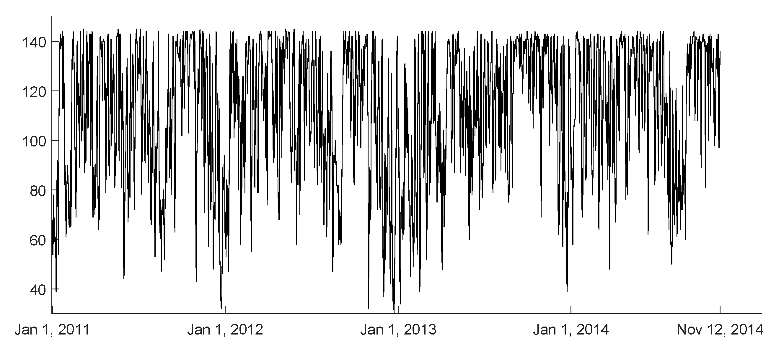
Hotel 1 and 2 are family-owned properties located on Lake Maggiore, a seasonal tourism destination in Northern Italy. The first is a five-star, 253-room hotel; the second is a four-star lodge with 128 rooms. Both properties are characterized by a seasonal closure between mid-October and early April: this feature has rarely been considered in hospitality research and explains the interest for the present analysis. Hotel 1 and 2 provided access to daily reservation data for three consecutive years, 2007–2009, during which special events were frequently hosted in the hotels themselves (wedding parties, conferences, business conventions) as well as in surrounding areas (exhibitions, sightseeing tours). These circumstances attracted a highly diversified customer base, including business/leisure and individual/group clients. Hotel 3 is a four-star city hotel in Milan, with 144 rooms. The hotel, which is open on a yearly basis, provided access to daily reservation data covering the period from 1 January 2011 to 12 November 2014 (approximately four years). Similar to hotels 1 and 2, hotel 3 also hosts a mixture of leisure and business customers, who are often attracted by special events (trade fairs, meetings and exhibitions) organized by the municipality throughout the year.
For all properties, the information stored in each reservation record includes the booking date, the arrival date, the (LOS) and the number of rooms booked. Although the customer base of the three hotels has a heterogeneous composition, an effective segmentation appears to be impracticable since guests’ characteristics often overlap (e.g., business guests may book either as individuals or corporate, arrive on a weekday for a business meeting and then stay over the weekend for a sightseeing tour or a cultural event). In this context, it seems more reasonable to aggregate all customers into a unique demand segment, as suggested in previous studies of small roadside hotels in the US [9] and small city hotels in Italy [15].
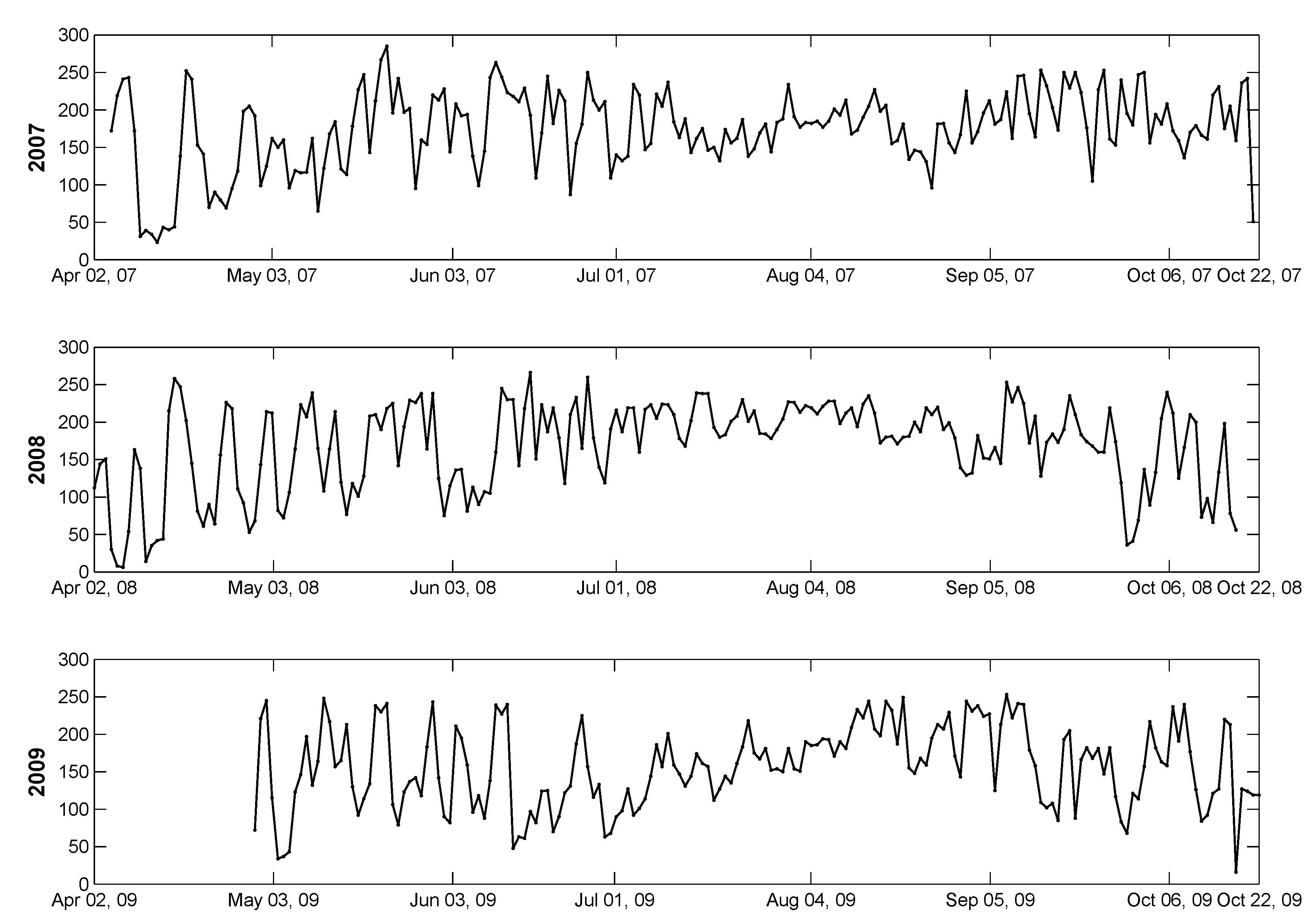
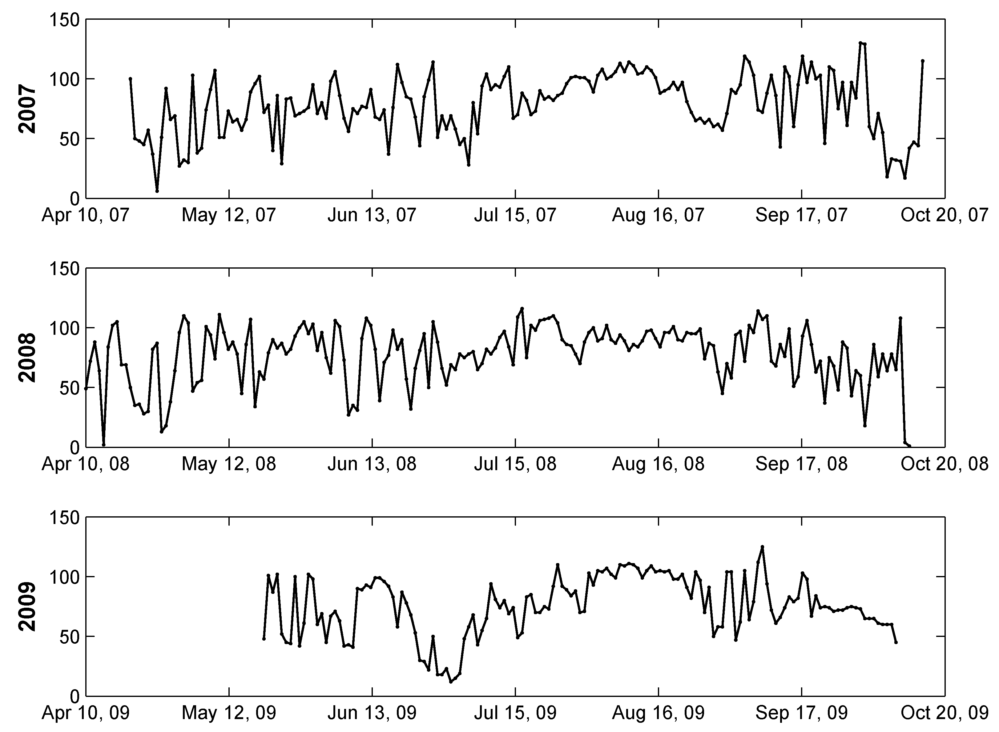
For hotel 1 and 2, each year in the sample period was processed separately, in consideration of the seasonal closures. The corresponding time series of daily room occupancy are shown, respectively, in Figure 1 and Figure 2. Figure 3 displays the (uninterrupted) time series of daily room occupancy for hotel 3 over the whole sample period. All figures exhibit significant peak-trough fluctuations, revealing that demand for all hotels is extremely volatile even in the short period.
A number of reasons were suggested in literature to explain why hospitality SMEs face a more volatile demand compared to their larger competitors. In addition to the presence of mixed clientele and special events as discussed above, these reasons include the inherent noise of reservation data, which are often recorded by staff with no specific training. These features make the task of forecasting demand for hospitality SMEs a very difficult one.
3.2. Forecasting Methods
Previous studies of hospitality SMEs in Italy [15,24] report the use of two types of demand forecasts, one based on historical booking data (long-term perspective) and the other based on advanced booking data (short-term perspective). Section 3.2.1 and Section 3.2.2 illustrate these methods and propose a few simple modifications to account for special events and LOS information.
As anticipated in Section 2, multiple studies have shown that there is no single best method for all cases and increasing model complexity does not necessarily produce more accurate forecasts. Therefore, the combination of different methods can be useful to reduce forecast errors, particularly when historical data are matched with recent booking data. In this regard, Section 3.3 introduces a performance-based weighting scheme that integrates the historical and the pickup method into a long-short forecast combination. Some measures of forecast accuracy, that will be used in the following analysis, are discussed in Section 3.4.
3.2.1. Historical Booking Forecasts
Daily series of hotel occupancy suggest that reservations behave similarly if they refer to the same calendar period and the same day-of-week. Therefore, the simplest occupancy forecast for a given day t (say, Wednesday, 18 July 2018) is the occupancy observed for the same day of the previous year (i.e., Wednesday, 19 July 2017). Formally,
where denotes the historical booking forecast of reservations for day-of-week d in week w of year and is the observed number of reservations received for the same day-of-week in the same week of the previous year. This naïve approach, known as “Same day-Last year” (SdLy), is often the only forecast implemented by hotel staff in small to medium-sized properties [24].
The main advantages of the SdLy method are minimal data requirements and ease of implementation. Nonetheless, a recent study [28] has shown that, in a number of circumstances, the performance of SdLy forecasts is comparable to that of more sophisticated time series models over multi-step-ahead forecast horizons.
A major shortcoming of SdLy forecasts is the use of a single data point, which may be subject to considerable noise. However, when SdLy is replaced by a simple average of occupancy levels on the same day of a few previous years, a substantial increase in forecast errors is possible [28]. A plausible explanation for these findings relates to the influence of special events that take place in the hotel itself, or in the destination. As the timing of such events varies from year to year, occupancy forecasts based on past years’ information may be seriously biased on specific days. A typical solution consists in regarding unusual days as outliers and removing them from the dataset. However, a long history of reservation data is needed to correctly apply outlier suppression techniques, and their impact on forecast quality is still controversial [15].
This study suggests an alternative approach that can be useful in the context of small seasonal hotels, in which the occupancy level is strongly dependent on special events that are already scheduled by the beginning of the current season (e.g., Easter, recurrent trade fairs, bank holidays). Based on publicly available information, the SdLy forecast for a day d in which a special event will take place in year can be replaced by the occupancy level recorded for the corresponding day of the same event in year . Conversely, the SdLy forecast for a day d in which no special events are scheduled for year can be replaced by the occupancy level in the nearest “ordinary” day-of-week in year . This modified SdLy approach, that is simply referred to as the historical (Hist) method in the rest of the paper, will be empirically tested in Section 4.
3.2.2. Advanced Booking Forecasts
Advanced booking methods exploit the daily records on how reservations are accumulating as time approaches the date of stay. Among them, the pickup techniques are the most commonly used. To forecast the arrivals on a future date, these methods integrate the number of bookings on hand on a given reading day with a quantity that is representative of the incremental bookings that will be “picked up” between the reading day and the stay night. Research in hospitality forecasting divides pickup methods into additive pickup (AP) and multiplicative pickup (MP). These are briefly described in the following paragraphs (for additional details, the interested reader is referred to, e.g., [14,25,29]). A step-by-step guide to reading reservation data and implementing pickup methods is provided in Appendix A.
Additive Pickup
In the AP, the number of reservations on hand is assumed to be independent of the total number of rooms sold. Hence, the final number of rooms booked for a given arrival day is estimated by adding the number of bookings accumulated until the current reading day to a sum of estimated pickup increments between consecutive lead times. Let denote the number of reservations received for the i-th check-in day at least j periods in advance, with indicating the reservation “lead time” (in particular, identifies the ”walk-ins”, i.e., customers who check-in without reserving in advance). Then, the difference
represents the net increment in bookings between lead times j and , for . On a reading day d, the k-period moving average
is the AP estimate of the expected pickup of rooms between lead times j and , for a future check-in day . For , a s-period-ahead forecast of the final number of reservations for t is computed by:
where denotes the latest cumulative bookings observable on the reading day d for the check-in day .
Multiplicative Pickup
The MP method assumes that the reservations on hand affect the rate of increase in room demand for future periods. Hence, the final number of reservations for a future check-in day is obtained by multiplying the number of bookings accumulated until the current reading day by a product of estimated pickup ratios between consecutive lead times.
Let denote the ratio between the number of rooms booked with lead times and j () for the i-th check-in day, then
On a reading day d, the hotel is interested in forecasting the total number of reservations for a future check-in day . Assuming that a volume-weighted average provides the most reliable results, the expected MP of bookings for t between lead times and j can be estimated by:
where is the length of the moving average. The s-period-ahead forecast of the final number of reservations for t is then computed by:
From Arrivals to Occupancy
A major limitation of all pickup methods is that they only forecast arrivals and not occupancy, since differences in LOS among the various reservations are not taken into account [16]. Nonetheless, LOS information impacts hotel occupancy and is a determinant of denials of booking attempts. Moreover, occupancy rates play a major role in hospitality RM as they guide hotel executives in deploying LOS controls in view of increasing occupancy on “shoulder” nights.
This study proposes a simple technique to incorporate LOS information directly into the reservations on hand in view of replacing the number of arrivals with the number of rooms effectively occupied by guests. Suppose that a hotel receives, j periods prior to a given arrival day t, a room reservation for r consecutive nights. It follows that the hotel occupancy for day t increases by one room as a consequence of a reservation received with lead time j; the occupancy for day increases by one room corresponding to one reservation with lead time ; and so on. Finally, the occupancy level for (the night before the departure) increases by one room corresponding to a reservation with lead time . In other words, one r-night reservation for arrival day t can be decomposed into r single-night reservations with different dates of stay (from t to ) and associated lead times (from j to ). Based on this decomposition, it is possible to re-define the cumulative bookings used in pickup Formulae (1) and (4) in such a way that now denotes the effective room occupancy rather than the number of arrivals. This information can be immediately processed by AP and MP algorithms to generate forecasts of future room occupancy based on Equations (3) and (6), respectively.
Calibration of AP and MP Averages
In practical applications of pickup methods, the most appropriate number of periods to include in moving averages of AP increments (2) or MP ratios (5) need to be determined. While some authors work with all the historical reservations available (see, e.g., [8]), others recommend the use of a limited amount (usually 3 to 6 weeks) of past data (see, e.g., [14]). Since the best solution appears to be context-specific, it is important to calibrate AP and MP estimates to optimize forecast quality in relation to the demand function faced by individual hotels. The approach proposed in the present study requires the creation of a training set of past reservation data. Based on the training set, the best number of periods to include in pickup averages can be determined by minimizing the Mean Square Error (MSE) of occupancy forecasts:
where denotes the true occupancy on day t, is the corresponding AP or MP forecast generated s-periods prior, n is the total number of such forecasts. The optimal obtained from the training set can subsequently be used to generate s-step-ahead forecasts of future room occupancy.
The proposed criterion is also related to the objectives of the next research stage. In particular, if the length of the pickup averages is calibrated by minimizing (7), it is then possible to use the minimum MSE at each forecast horizon to determine a performance-based weighting for the pickup component in the forecast combinations. This proposal is illustrated in the next section.
3.3. Performance-Based Combinations
Individually, pickup and historical booking forecasts track the dynamics of different time scales. As argued in Andrawis et al. [26], combining two methods based on diverse information sources can substantially reduce the forecast error variance, leading to a forecast quality which is often superior to that of either method on its own.
Ways to best combine forecasts have been widely investigated. A simple but effective approach consists in applying a dynamic weighting scheme that is updated according to the number of steps ahead being forecast. When the date of stay is far into the future, more weight should be assigned to the historical booking method, which is based on a long-term perspective. Conversely, the pickup method, which is more reactive to recent demand shifts, should have a greater influence on the forecast combination when the date of stay is imminent [15]. Another well-established approach consists in weighting each constituent method according to its historical performance. Thus, more weight should be put on methods that have produced relatively more accurate forecasts in the recent past [23].
This work proposes a new combination strategy that is both performance- and time-weighted. Denote by the actual occupancy on a given day t and by a forecast of generated s periods prior by method i. Here, any pickup method (AP or MP) is identified by and the historical booking method by . Based on a training set of data, the performance of each method at forecast horizon s is evaluated by the corresponding MSE:
where n is the total number of s-step-ahead forecasts available. Assuming that the ratio of over is approximately stable over time, a combined s-step-ahead occupancy forecast for a future day t can be defined by:
where
denotes the relative weight of the first constituent (pickup) and is the relative weight of the second constituent (historical booking).
The outcome of this approach is a performance-based weighting scheme tailored to the forecast horizon. As time nears the date of stay, the forecast combination adapts dynamically to changes in the relative performance of the constituent methods. More details on estimation and empirical results are given in Section 4.
3.4. Forecast Accuracy
In addition to the MSE, several measures of forecast accuracy have been used in literature to compare the performance of alternative forecasting methods (see, e.g., [11] for a comprehensive study). Based on the forecast error
the following accuracy metrics will be used in Section 4 to evaluate multiple aspects of forecast quality:
- Mean Absolute Error (MAE):The measure is expressed in the same scale (= number of rooms) as the data, thus allowing a direct evaluation of losses associated to forecast errors
- Mean Absolute Scaled Error (MASE):This is a scale-free metric with denominator given by the in-sample MAE of a naïve method, the one-step-ahead random walk. The measure is easily interpreted as the relative performance gain (MASE ) or loss (MASE ) of the proposed approach compared to the naïve method. It can be used to compare forecast methods on a single demand series (like MAE) and also to compare forecast accuracy between series.
- Mean Absolute Percentage Error (MAPE):This is the percentage-error measure most frequently used in practice: it is meaningful to decision makers, easy to communicate and useful in comparing forecasts from different situations.
In real-world circumstances, hotel room occupancy has to be predicted and re-predicted multiple times as the date of stay approaches. Forecasts computed several weeks in advance allow Revenue Managers to plan marketing strategies that could be implemented in response to possible low-demand periods, usually in cooperation with the sales team. Conversely, short-term forecasts (with a lead time of one or two weeks) are instrumental to choices among a few tactical options (such as adjusting inventory controls). It is consequently crucial for an effective demand management system to evaluate the accuracy of a forecasting method separately at a number of different forecast horizons and to monitor how accuracy evolves as the date of stay approaches. This dynamic perspective is adopted in the empirical analysis presented in the next section.
4. Results
The datasets described in Section 3.1 were used to test AP and MP individually, and then in combination with the historical (Hist) method according to the performance-based criterion described in Section 3.3.
4.1. Preliminary Analysis
Since the data reservation patterns and volumes exhibit a strong weekly seasonality, the forecasting problem was separated by day-of-week as is common practice in the hotel industry [9]. For each year in the sample period, arrivals were combined with LOS information to generate seven occupancy matrices, each reflecting the buildup of reservations on a specific weekday. The occupancy matrix of past Mondays was then used to forecast occupancy on future Mondays, and so on.
Occupancy records were compared to the capacity of each hotel to detect possible outliers and inconsistencies in the data. When the occupancy exceeded the hotel capacity, the corresponding data were adjusted to reflect the effective number of rooms available in each hotel. Following Ellero and Pellegrini [15], no other outlier suppression technique was applied since using effective reservation records appeared to improve the quality of pickup forecasts.
The study was divided in two stages. Forecasts of daily room occupancy for a specific date were computed six times before the date, using forecast horizons s of one to six weeks ahead. In the first stage, data from 2007–2008 (hotel 1 and 2) and from 2011–2013 (hotel 3) were used as a training set to calibrate values of the forecast parameters and for weeks (forecast horizon). In the second stage, data from 2009 (hotel 1 and 2) and from 2014 (hotel 3) were used as an evaluation set to compare the accuracy of individual and combined forecasting methods. For hotel 1, the forecasting period was chosen to cover all dates between July, 1 (beginning of high season) and 12 October, yielding a total number of 104 daily occupancy forecasts for each forecast horizon. For hotel 2, in view of the later seasonal opening, the forecast period was shifted to 15 July–22 October (100 forecasts for each forecast horizon). For hotel 3, thanks to the availability of an uninterrupted time series, it was possible to obtain 316 daily occupancy forecasts for each forecast horizon, covering the period from 1 January to 12 November.
All calculations can be performed in a worksheet environment, with minimal training.
4.2. Stage 1: Calibrating Forecast Parameters
4.2.1. Pickup Averages
Based on the training set, AP and MP forecasts were computed with different amounts of sample data ( weeks, possibly subject to data availability). The best number of periods to include in pickup calculations was determined separately for each forecast horizon according to the lowest MSE of occupancy forecasts (7). Table 1 illustrates the results (the table refers to year 2008 for hotels 1 and 2, and to pooled years 2011–2013 for hotel 3).
For seasonal hotels 1 and 2, both pickup methods displayed similar error patterns. Pickup forecasts based on short moving averages ( weeks of sample data) performed generally better over short forecast horizons. Conversely, as the forecast horizon increased, the MSE decreased monotonically with k for both hotels, independently of the pickup method in use. In particular, the optimal calibration of pickup forecasts required the maximum amount of sample data available in the training set when the forecast horizon exceeded, respectively, 2 weeks for hotel 1 and 3 weeks for hotel 2. For hotel 3, AP was considerably more accurate than MP. For both methods, the optimal length of pickup averages was equal to 16 weeks across all forecast horizons.
4.2.2. Performance-Based Weights for Combined Forecasts
For seasonal hotels 1 and 2, Hist forecasts for the year 2008 were generated from 2007 occupancy data using the SdLy method adjusted for calendar effects and public information available at least six weeks before the date of stay. For hotel 1, the Hist method performed sensibly worse than both pickup methods, with a square root of the MSE close to 63 rooms. Conversely, for hotel 2, the square root of the MSE for Hist forecasts was equal to 27.46, not far from the performances of AP (24.99) and MP (27.60) over a 6-week forecast horizon (cf. Table 1).
For hotel 3, based on the availability of a longer and uninterrupted time series, the Hist method for a given day-of-week d in 2013 was implemented by averaging the occupancy levels on the corresponding day-of-week for years 2011 and 2012. This gave a square root of the MSE for Hist forecasts equal to 28.53, considerably worse than AP but more accurate than MP over forecast horizons exceeding 2 weeks.
Assuming that the MSE ratio between Hist and pickup forecasts is approximately stable over time in each hotel, the MSE estimates obtained for AP, MP and Hist over the training set were used to calibrate the weights of forecast combinations for future years, as explained in Section 3.2.2. In particular, the MSE estimates retained for AP and MP were those corresponding to the best-performing pickup calibrated to each forecast horizon (Table 1). These MSEs were combined with those of Hist forecasts according to the weighting scheme given in Equation (8). The first constituent forecast (to be assigned weight ) was identified with either AP or MP, the second constituent (with weight ) was identified with Hist. The outcome of this approach, shown in Table 2, was a performance-based weighting scheme that varied according to the forecast horizon. As the occupancy date moved far into the future, more and more weight was attributed to the Hist component, whereas when the occupancy date became imminent, more and more weight was put on pickup forecasts. For seasonal hotels 1 and 2, this time-varying structure appears to be influenced by the choice of the pickup method only to a limited extent, as was slightly higher for AP compared to MP. The relative weight of the Hist constituent was quite relevant for hotel 2, in which the performance of this method was comparable to that of pickup forecasts. Conversely, for hotel 1, the weight attributed to the Hist constituent never exceeded , even at the longest forecast horizons. Interestingly, for hotel 3, the weight attributed to the Hist component was sensibly higher in combination with MP, since Hist forecasts outperformed MP forecasts considerably for over the training period.
4.3. Stage 2: Evaluating Forecast Accuracy
In the second stage of the empirical study, the accuracy of individual pickup forecasts (AP, MP) and combined pickup/historical forecasts was tested on the evaluation set. In addition to forecast combinations with performance-based weights, the study includes a simple combination assigning weight to both Hist and pickup forecasts, irrespective of the forecast horizon. The different combinations are identified by the following notation: AP-S (respectively, MP-S) denotes the simple, equally weighted average of additive (respectively, multiplicative) pickup and Hist forecasts; AP-W (MP-W) is the performance-weighted combination of additive (multiplicative) pickup and Hist forecasts.
In order to compare the accuracy of the proposed methods with a commonly used benchmark, a simple moving average (MA) of length was used:
where is the one-step-ahead MA forecast computed by averaging the last m records of observed demand for a specific day-of-week d. Based on preliminary analysis performed on the training set, the parameter m was set equal to 3 for hotels 1 and 2, and 5 for hotel 3.
For each forecast horizon s ( weeks), the best performing method was identified as that delivering, on average, the lowest forecast error according to the accuracy metrics described in Section 3.4. The outcomes of the different metrics (MAE, MASE and MAPE) are summarized in Table 3, Table 4 and Table 5, respectively for hotel 1, 2 and 3. At every forecast horizon, the best and worst method(s) were compared (the simple moving average (MA) was not included in this comparison because it was not used in forecast combinations (it was just included in Table 3, Table 4 and Table 5, as a benchmark model)) for each hotel and the percentage reduction in forecast errors from the worst to the best method was averaged across the various accuracy measures (Table 6).
These findings indicate that, with the only exception of hotel 3 for a forecast horizon of 6 weeks, the most accurate method was always a pickup/historical combination with performance-based weights. For hotel 1, the combination included AP at short forecast horizons ( weeks) and MP at longer horizons ( weeks). For hotel 2, the MP-W combination was optimal for weeks, whereas AP-W performed better at any other forecast horizon. For hotel 3, AP-W was optimal for and AP-S for . According to the tables, the best-performing combinations had MASE between and for hotel 1, between and for hotel 2, between 0.42 and 64 for hotel 3. These numbers represent much better forecasts, on average, relative to one-step ahead, naïve forecasts computed in sample.
Looking at the forecast-quality of individual pickup methods, MP appears globally more accurate than AP for hotel 1 but (considerably) less accurate for hotel 2 and 3. Hence, the choice between additive and multiplicative pickup is to be considered a context-specific issue. Moreover, performance differences between forecast combinations and individual pickup methods were particularly evident over forecast horizons exceeding 3 weeks: for hotel 1, the performance improvement from the worst pickup (AP) to the best combined forecast (MP-W) was between and ; for hotel 2, MP (worst pickup) was outperformed by AP-W (best combination) by a factor of 39.3%–50.1%; for hotel 3, AP-W improved over MP by a factor of 21.8%–53.8% (Table 6).
The simple average of Hist and pickup forecasts was frequently among the worst-performing methods. In particular, for hotel 1 and weeks, the use of performance-based weights led to an improvement in forecast accuracy in the order of 27%–65% relative to equally weighted combinations. These findings suggest that choosing an appropriate weighting scheme for combined forecasts is crucial to forecast accuracy, particularly when constituent methods have different individual performances.
A further advantage of combining forecasts with different time frames emerges from the last two columns in Table 6. The forecast error correlation between Hist and pickup was frequently close to zero (and sometimes negative), indicating that forecast errors made by the two methods (partly) offset each other. In practice, when the historical method overestimated occupancy on a given date, the pickup method frequently underestimated it (and vice versa). As a consequence, the performance-weighted combination of Hist and pickup forecasts was able to deliver good quality forecasts even in situations when the Hist method (hotel 1), or the MP method (hotel 3), had a rather poor individual performance.
5. Discussion
The ability to forecast and, possibly, control demand fluctuations is crucial to the development of tourism sustainability. Mismatching of supply and demand, with consequent over- or under-utilization of capacity, are characteristic features of the tourist industry that threaten, in particular, small and medium-sized seasonal hotels. Even if “for some hotels seasonal closure may continue to be the most cost-effective method for dealing with pronounced seasonality” ([30], p. 138), nonetheless these hotels may focus on improving occupancy levels during intermediate, or “shoulder”, seasons and attempting to extend the main season. In particular, “the occupancy analysis needs to be performed at the individual hotel level, and marketing plans to counteract seasonality should be tailor-made to suit the particular occupancy performance patterns and precise circumstances of the individual hotels involved” ([30], p. 139).
The present study has focused on forecasting occupancy for hospitality SMEs, in which occupancy levels are strongly dependent on external events and reservation data are difficult to handle due to a variety of reasons (seasonal interruptions, sparse information, intrinsic noise). In a context of growing global tourism markets, the ability to understand and anticipate the pattern of future demand represents a competitive advantage for hospitality SMEs, since it is directly related to the opportunity of designing effective demand-side policies as a response to dynamic changes in tastes and customer habits.
As recommended by Koupriouchina et al. [11], the study was designed in relation to multiple criteria, including data characteristics, practical implications of the forecasts, and the nature of decisions derived from them. The proposed approach was tested on real reservation data provided by three independent hotels in Northern Italy (one in Milan and two on Lake Maggiore, a seasonal tourism destination). Whereas most of the hospitality forecasting research was conducted on large international hotels and hotel chains, this data set is valuable also for low-volume, small to medium-sized businesses, two of which are family-owned and operated on a seasonal basis. In all cases, our forecast combination model performed better than the competing methods in terms of various error measures (MAE, MASE, MAPE). These findings were (partly) expected since the combination of forecasting techniques has long been a key direction of methodological development and a number of authors have shown that forecast combinations are a robust approach to reduce the risk of large forecast errors ( see, e.g., Wu et al. [23] and the references therein).
5.1. Theoretical Implications
In addition to validating earlier findings about combinations of long-term and short-term forecasts [26], the present work makes the point that using performance-based weights improves forecast accuracy.
A peculiarity of the forecast combinations proposed here is that the weights are updated weekly according to the relative forecast errors made by the short- and long-term constituent methods over specific forecast horizons. This gives a performance-based weighting scheme that adapts dynamically to the characteristics of demand functions experienced by the individual hotel. In particular, performance improvements between and relative to the MAPE of individual pickup methods were observed in the empirical study (Section 5). A further explanation for these findings relates to the fact that forecast errors made by historical and pickup methods were nearly uncorrelated. Hence, combining these forecasts with performance-based weights was a good strategy to take advantage of (partial) compensations between negative and positive forecast errors made by each constituent method. This effect was so relevant that it largely offset some inaccuracies of historical booking forecasts (hotel 1 and 2) and MP forecasts (hotel 3).
In view of the importance of occupancy forecasting for implementing effective LOS policies, the current study has introduced a simple method that integrates LOS information into the partially accumulated reservations on hand. This generates occupancy-based reservation records that can be used as inputs to conventional pickup methods. As shown in Table 3, Table 4 and Table 5, the proposed approach yields accurate pickup forecasts of hotel occupancy. In particular, averaging the MAE of the best pickup method over all forecast horizons gives a value of 23 for hotel 1 (253 rooms), 13 for hotel 2 (128 rooms) and 16 for hotel 3 (144 rooms), which represents a considerable improvement in terms of forecast accuracy relative to previous studies of small city hotels in Italy [15] and in the US [9].
5.2. Practical Implications
These findings underscore the importance that small to medium-sized hotels develop their own demand forecasting systems combining internal resources with external information concerning special events. As different businesses face different demand functions, the present study suggests that managers in hospitality SMEs should carry out an empirical analysis on the hotel’s own data. In particular, a training set of (at least) two years of reservation records should be collected in view of (a) testing the performance of long-term and short-term forecasting methods, (b) identifying which methods generate the lowest correlation between forecast errors and (c) calibrating performance-based weights to use in forecast combinations. Since timeliness is crucial to effective demand fulfillment policies, the quality of individual and combined forecasts should be evaluated separately at different forecast horizons (cf. [11]). As shown in the empirical study, this approach produces dynamic adjustments in forecast combinations that can be helpful in capturing extreme demand fluctuations experienced by small and medium-sized hotels.
Given that SMEs likely have limited access to technology and usually lack well-trained RM personnel, the proposed models were designed for execution in a worksheet environment with minimal training. It is nevertheless crucial to collect detailed customer information inside each organization, and to carry out basic investments in human resources to achieve the competitive advantage that can arise from increased productivity and managerial efficiency [31]. In this perspective, collaboration with local authorities in reservation management and event planning appears to be a relevant direction for sustainable development of the sector [1,4].
5.3. Limitations and Future Research
Although the proposed methodology leads to a number of practical implications, it should be remembered that the current investigation is based on hotel-specific data provided by three establishments for a limited period of time. Further empirical work is needed to develop a more thorough understanding of specific demand features and possibly identify more sophisticated strategies that could be implemented in the context of hospitality SMEs. In particular, a number of socio-economic factors (including income, prices, exchange rates, marketing spending, infrastructures, tastes and preferences) influence tourism demand at an aggregate level. The potential impact of these factors on demand patterns for hospitality at a single-establishment level certainly deserves further investigation.
Since occupancy levels appear to be strongly influenced by special events (trade fairs, international holidays, exhibitions, ⋯), future research could focus on the impact of collaborative networks and public-private coordination in promoting off-season visits and possible season extensions [1,32].
In addition to external information about special events, managers of small and medium-sized hotels are encouraged to collect internal information about customers’ countries of origin and/or reservation channels (web, travel agencies, ⋯). These data could be used to identify and forecast specific demand segments, offering a concrete alternative to the classical distinction between business and leisure clients that is of little use in hospitality SMEs [9,15].
6. Conclusions
This study has investigated the application of demand forecasting models to hospitality SMEs, based on hotel-specific data. The proposed models feature a combination of historical and advanced booking forecasts, which are easily implemented in a worksheet environment and are compatible with seasonal interruptions in reservation data. Empirical results obtained for three Italian hotels show a considerable improvement in forecast accuracy compared to commonly used methods (such as simple moving average). These findings underscore the importance of being able to forecast in the hospitality sector in view of gaining a competitive advantage. In particular, the proposed approach could help small and medium-sized hotels to develop effective demand-side policies, with the ultimate purpose of enhancing their sustainable development.
Author Contributions
The authors have contributed equally to research design and development, data analysis, and writing the paper.
Funding
This research received no external funding.
Conflicts of Interest
The authors declare no conflict of interest.
Abbreviations
The following abbreviations are used in this manuscript:
| AP | Additive pickup |
| AP-S | Equally weighted average of additive pickup and Hist forecasts |
| AP-W | Performance-weighted average of additive pickup and Hist forecasts |
| Hist | Historical |
| LOS | Length-of-stay |
| MAE | Mean Absolute Error |
| MASE | Mean Absolute Scaled Error |
| MASE | Mean Absolute Percentage Error |
| MP | Multiplicative pickup |
| MP-S | Equally weighted average of multiplicative pickup and Hist forecasts |
| MP-W | Performance-weighted average of multiplicative pickup and Hist forecasts |
| SMEs | Small and Medium Enterprises |
Appendix A
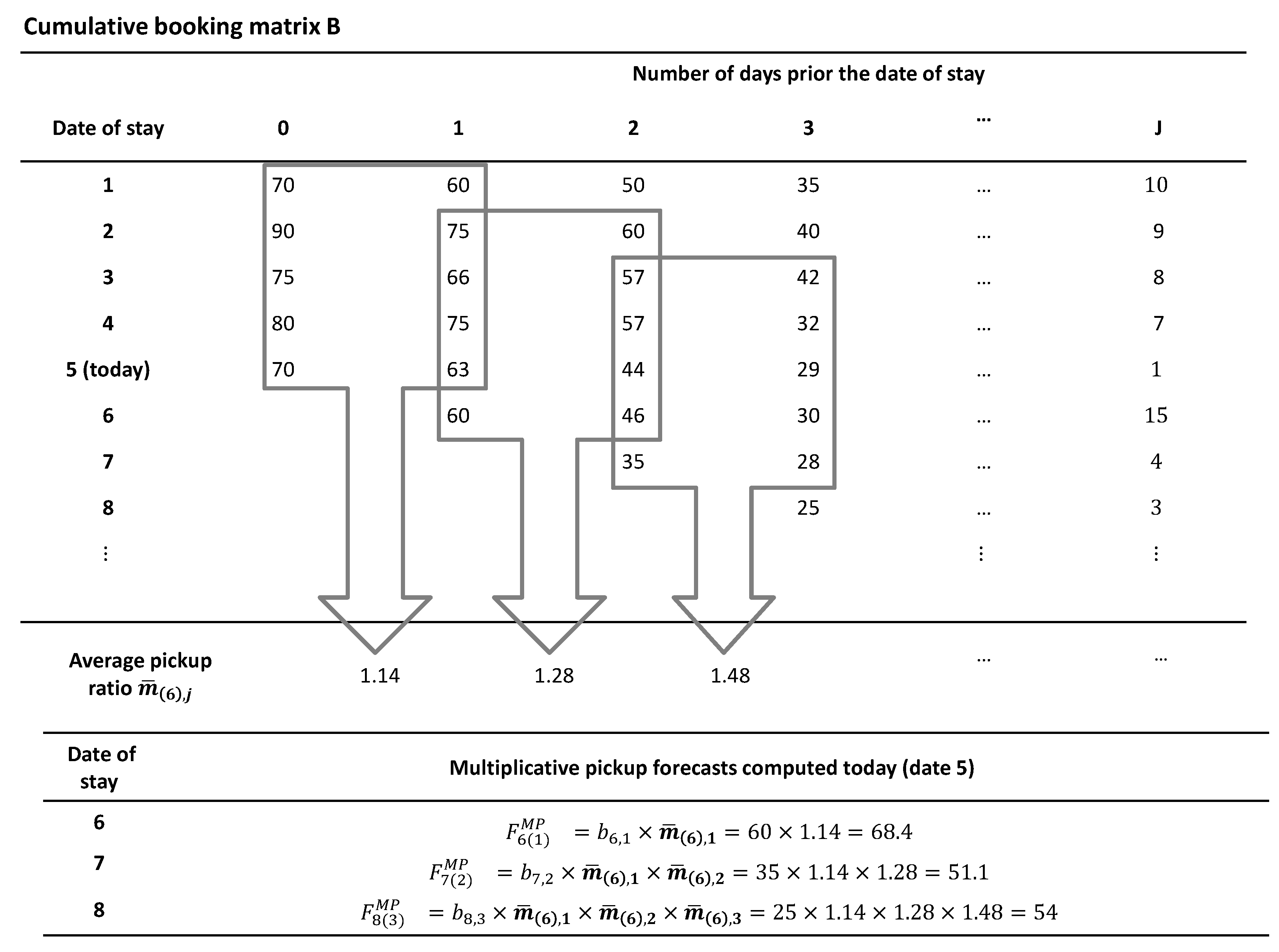
Appendix A.1. The Cumulative Booking Matrix
Let denote the number of reservations received for the i-th check-in day at least j periods (days or weeks) in advance, with indicating the reservation “lead time” (in particular, identifies the “walk-ins”, i.e., customers who check-in without reserving in advance). This information can be summarized into a cumulative booking matrix . The structure of this matrix is illustrated by a numerical example in the following table, where today is represented by row and future dates have to be forecast.
The information contained in Table A1 can be read as follows. On date 5 (today), 70 rooms were reserved by walk-in customers (), 63 rooms were reserved at least one period in advance , 44 rooms were reserved at least two periods in advance , and so on. For tomorrow , information is available for rooms that have been reserved at least one period in advance, for information is available for rooms that have been reserved at least two periods in advance, and so on. Advanced booking models use reservation data from the cumulative matrix B both for completed stay nights and for stay nights which have not yet occurred , since partially accumulated bookings are nonetheless available.

Table A1.
Cumulative booking matrix, a numerical example.
| Number of Days Prior to Date of Stay | ||||||
|---|---|---|---|---|---|---|
| Date of Stay | 0 | 1 | 2 | 3 | ⋯ | J |
| 1 | 70 | 60 | 50 | 35 | 10 | |
| 2 | 90 | 75 | 60 | 40 | 9 | |
| 3 | 75 | 66 | 57 | 42 | 8 | |
| 4 | 80 | 75 | 57 | 32 | 7 | |
| 5 (today) | 70 | 63 | 44 | 29 | ⋯ | 1 |
| 6 | − | 60 | 46 | 30 | 15 | |
| 7 | − | − | 35 | 28 | 1 | |
| 8 | − | − | − | 25 | ⋯ | 3 |
Appendix A.2. Multiplicative Pickup (MP)
For multiplicative pickup (MP), the information given in consecutive columns of B is used to compute the average pickup ratio between consecutive booking periods, according to Equation (5). This is illustrated in Figure A1, where the elements in the numerator and denominator of each pickup ratio are included in a gray rectangle. The one-period-ahead pickup ratio, denoted by , is multiplied by 60 (the bookings on hand for day 6) to obtain the MP forecast of rooms for . The product of two consecutive pickup ratios, and , is multiplied by 35 to obtain the MP forecast of rooms for (two-period-ahead). Finally, the product , and is multiplied by 25 to derive the MP forecast of rooms for (three-period-ahead).
Figure A1.
Derivation of MP forecasts for dates , based on (complete and incomplete) booking information available today .
Figure A1.
Derivation of MP forecasts for dates , based on (complete and incomplete) booking information available today .

Appendix A.3. Additive Pickup (AP)
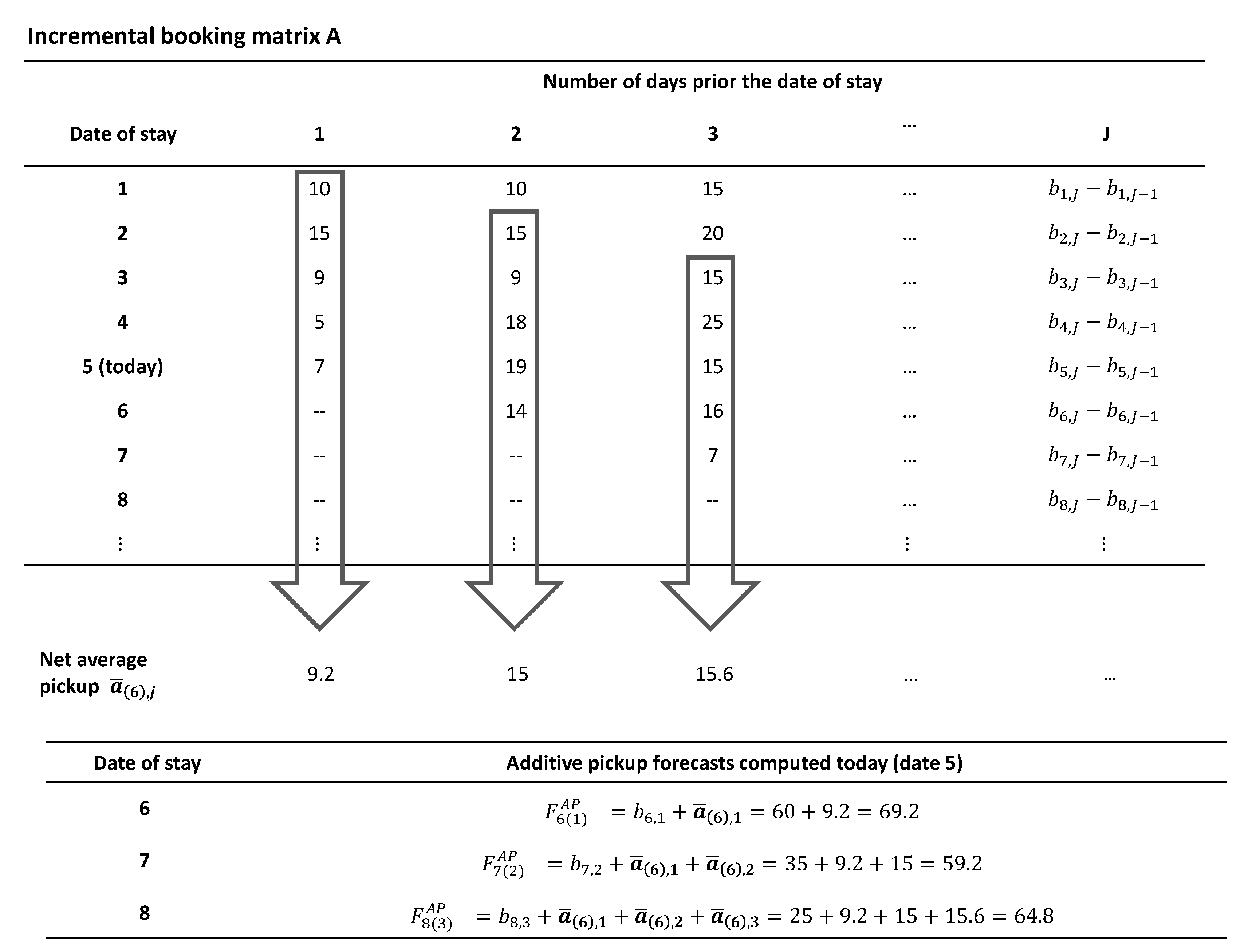
The derivation of additive pickup (AP) forecasts starts from the incremental booking matrix A, which is obtained by subtracting consecutive columns of matrix B as explained in Equation (1) and illustrated here in Figure A2. Simple moving averages of incremental bookings are computed to estimate the expected pickup of rooms between consecutive booking dates, according to Equation (2). The figure illustrates these calculations for a pickup average of length , yielding the net average pickup increments denoted by . Adding these increments to the latest bookings on hand for a particular stay date gives the AP forecast of rooms for the corresponding date, as shown in the figure.
Figure A2.
Derivation of AP forecasts for dates , based on (complete and incomplete) booking information available today .
Figure A2.
Derivation of AP forecasts for dates , based on (complete and incomplete) booking information available today .

References
- UNEP and WTO. Making Tourism More Sustainable: A Guide for Policy Makers; United Nations Environment Programme: Paris, France; World Tourism Organization: Madrid, Spain, 2005. [Google Scholar]
- Svetlačić, R. Aspects of Sustainable Development of Small and Family Hotels. In Economic and Social Development: Book of Proceedings; Varazdin Development and Entrepreneurship Agency: Varazdin, Croatia, 2016; pp. 2–11. [Google Scholar]
- Mihalič, T.; Žabkar, V.; Cvelbar, L.K. A hotel sustainability business model: Evidence from Slovenia. J. Sustain. Tour. 2012, 20, 701–719. [Google Scholar] [CrossRef]
- European Commission. Yield Management in Small and Medium-Sized Enterprises in the Tourism Industry: General Report; Office for Official Publications of the European Communities: Luxembourg, 1997. [Google Scholar]
- Cucculelli, M.; Goffi, G. Does sustainability enhance tourism destination competitiveness? Evidence from Italian Destinations of Excellence. J. Clean. Prod. 2016, 111, 370–382. [Google Scholar] [CrossRef]
- Liu, Z. Sustainable tourism development: A critique. J. Sustain. Tour. 2003, 11, 459–475. [Google Scholar] [CrossRef]
- Liu, Z. Tourism development—A system analysis. In Tourism: The State of the Art; Seaton, A., Ed.; John Wiley: Chichester, UK, 1994; pp. 20–30. [Google Scholar]
- Talluri, K.T.; Van Ryzin, G.J. The Theory and Practice of Revenue Management; Springer Science & Business Media: Berlin/Heidelberg, Germany, 2006; Volume 68. [Google Scholar]
- Weatherford, L.R.; Kimes, S.E. A comparison of forecasting methods for hotel revenue management. Int. J. Forecast. 2003, 19, 401–415. [Google Scholar] [CrossRef]
- Donaghy, K.; McMahon-Beattie, U.; McDowell, D. Implementing yield management: Lessons from the hotel sector. Int. J. Contemp. Hosp. Manag. 1997, 9, 50–54. [Google Scholar] [CrossRef]
- Koupriouchina, L.; van der Rest, J.P.; Schwartz, Z. On revenue management and the use of occupancy forecasting error measures. Int. J. Hosp. Manag. 2014, 41, 104–114. [Google Scholar] [CrossRef]
- Lee, M. Modeling and forecasting hotel room demand based on advance booking information. Tour. Manag. 2018, 66, 62–71. [Google Scholar] [CrossRef]
- Uysal, M.; Schwartz, Z.; Sirakaya-Turk, E. Management Science Applications in Tourism and Hospitality; CRC Press: Boca Raton, FL, USA, 2017. [Google Scholar]
- Zeni, R.H. Improved Forecast Accuracy in Airline Revenue Management by Unconstraining Demand Estimates from Censored Data; Universal Publishers: Irvine, CA, USA, 2001. [Google Scholar]
- Ellero, A.; Pellegrini, P. Are traditional forecasting models suitable for hotels in Italian cities? Int. J. Contemp. Hosp. Manag. 2014, 26, 383–400. [Google Scholar] [CrossRef]
- Zakhary, A.; Atiya, A.F.; El-Shishiny, H.; Gayar, N.E. Forecasting hotel arrivals and occupancy using Monte Carlo simulation. J. Revenue Pricing Manag. 2011, 10, 344–366. [Google Scholar] [CrossRef]
- Bails, D.; Peppers, L.C. Business Fluctuations: Forecasting Techniques and Applications; Prentice Hall: Upper Saddle River, NJ, USA, 1993. [Google Scholar]
- Croes, R.R. Anatomy of Demand in International Tourism: The Case of Aruba; Uitgeverij Van Gorcum: Assen, The Netherlands, 2000. [Google Scholar]
- Goh, C. Exploring impact of climate on tourism demand. Ann. Tour. Res. 2012, 39, 1859–1883. [Google Scholar] [CrossRef]
- Witt, S.F.; Song, H.; Li, G. The Advanced Econometrics of Tourism Demand; Routledge: London, UK, 2008. [Google Scholar]
- Zakhary, A.; El Gayar, N.; Atiya, A.F. A comparative study of the pickup method and its variations using a simulated hotel reservation data. ICGST Int. J. Artif. Intell. Mach. Learn. 2008, 8, 15–21. [Google Scholar]
- Lim, C.; Chang, C.; McAleer, M. Forecasting h (m) otel guest nights in New Zealand. Int. J. Hosp. Manag. 2009, 28, 228–235. [Google Scholar] [CrossRef]
- Wu, D.C.; Song, H.; Shen, S. New developments in tourism and hotel demand modeling and forecasting. Int. J. Contemp. Hosp. Manag. 2017, 29, 507–529. [Google Scholar] [CrossRef] [Green Version]
- Luciani, S. Implementing yield management in small and medium sized hotels: An investigation of obstacles and success factors in Florence hotels. Int. J. Hosp. Manag. 1999, 18, 129–142. [Google Scholar] [CrossRef]
- Ivanov, S. Hotel Revenue Management: From Theory to Practice; Zangador: Varna, Bulgaria, 2014. [Google Scholar]
- Andrawis, R.R.; Atiya, A.F.; El-Shishiny, H. Combination of long term and short term forecasts, with application to tourism demand forecasting. Int. J. Forecast. 2011, 27, 870–886. [Google Scholar] [CrossRef]
- Rajopadhye, M.; Ghalia, M.B.; Wang, P.P.; Baker, T.; Eister, C.V. Forecasting uncertain hotel room demand. Inf. Sci. 2001, 132, 1–11. [Google Scholar] [CrossRef]
- Pereira, L.N. An introduction to helpful forecasting methods for hotel revenue management. Int. J. Hosp. Manag. 2016, 58, 13–23. [Google Scholar] [CrossRef]
- Phumchusri, N.; Mongkolkul, P. Hotel room demand forecasting via observed reservation information. In Proceedings of the Asia Pacific Industrial Engineering and Management Systems Conference, Phuket, Thailand, 3–5 December 2012; pp. 1978–1985. [Google Scholar]
- Jeffrey, D.; Barden, R.R. An analysis of the nature, causes and marketing implications of seasonality in the occupancy performance of English hotels. Tour. Econ. 1999, 5, 69–91. [Google Scholar] [CrossRef]
- Pappas, N. Achieving competitiveness in Greek accommodation establishments during recession. Int. J. Tour. Res. 2015, 17, 375–387. [Google Scholar] [CrossRef]
- Marasco, A.; De Martino, M.; Magnotti, F.; Morvillo, A. Collaborative innovation in tourism and hospitality: A systematic review of the literature. Int. J. Contemp. Hosp. Manag. 2018, 30, 2364–2395. [Google Scholar] [CrossRef]
Figure 1.
Hotel 1, time series of daily room occupancy for years 2007 (top), 2008 (center), 2009 (bottom).
Figure 1.
Hotel 1, time series of daily room occupancy for years 2007 (top), 2008 (center), 2009 (bottom).

Figure 2.
Hotel 2, time series of daily room occupancy for years 2007 (top), 2008 (center), 2009 (bottom).
Figure 2.
Hotel 2, time series of daily room occupancy for years 2007 (top), 2008 (center), 2009 (bottom).

Figure 3.
Hotel 3, time series of daily room occupancy from 1 January 2011 to 12 November 2014.

Table 1.
Best amount of weekly data to include in pickup averages, respectively for additive pickup (AP) and multiplicative pickup (MP), by forecast horizon s (with s ranging from one to six weeks prior to the date of stay). In brackets: square root of the minimum Mean Square Error (MSE).
Table 1.
Best amount of weekly data to include in pickup averages, respectively for additive pickup (AP) and multiplicative pickup (MP), by forecast horizon s (with s ranging from one to six weeks prior to the date of stay). In brackets: square root of the minimum Mean Square Error (MSE).
| Hotel 1 | Hotel 2 | Hotel 3 | ||||||
|---|---|---|---|---|---|---|---|---|
| s | AP | MP | s | AP | MP | s | AP | MP |
| 1 | 3 (14.93) | 3 (15.93) | 1 | 2 (7.91) | 3 (8.84) | 1 | 16 (16.47) | 16 (20.53) |
| 2 | 2 (25.71) | 2 (27.45) | 2 | 2 (11.81) | 2 (13.37) | 2 | 16 (20.81) | 16 (29.48) |
| 3 | 10 * (36.36) | 10 * (37.02) | 3 | 2 (16.41) | 2 (17.33) | 3 | 16 * (21.93) | 16 (33.43) |
| 4 | 9 * (42.91) | 9 * (45.45) | 4 | 10 * (22.38) | 10 * (24.48) | 4 | 16 * (22.98) | 16 (37.17) |
| 5 | 8 * (47.23) | 8 * (49.90) | 5 | 9 * (24.43) | 9 * (26.94) | 5 | 16 * (23.06) | 16 (39.52) |
| 6 | 7 * (51.99) | 7 * (56.86) | 6 | 8 * (24.99) | 8 * (27.60) | 6 | 16 * (23.18) | 16 (44.99) |
* The MSE was monotonically decreasing as the number of weekly data used in pickup forecasts increased. In these circumstances, the minimum MSE was reached by the longest pickup average compatible with the sample size, given the forecast horizon.
Table 2.
Percentage weights for performance-based combinations of pickup and historical booking (Hist) forecasts, according to the forecast horizon s (from 1 to 6 weeks). AP denotes Additive Pickup, MP denotes Multiplicative Pickup.
Table 2.
Percentage weights for performance-based combinations of pickup and historical booking (Hist) forecasts, according to the forecast horizon s (from 1 to 6 weeks). AP denotes Additive Pickup, MP denotes Multiplicative Pickup.
| Hotel 1 | ||||||
| s | 1 | 2 | 3 | 4 | 5 | 6 |
| AP | 94.49 | 86.35 | 74.58 | 68.09 | 64.61 | 61.07 |
| Hist | 5.51 | 13.65 | 25.42 | 31.91 | 35.39 | 38.93 |
| MP | 91.78 | 83.94 | 69.95 | 61.48 | 58.73 | 54.03 |
| Hist | 8.22 | 16.06 | 30.05 | 38.52 | 41.27 | 45.97 |
| Hotel 2 | ||||||
| s | 1 | 2 | 3 | 4 | 5 | 6 |
| AP | 92.35 | 84.28 | 55.66 | 43.76 | 42.98 | 40.76 |
| Hist | 7.65 | 15.72 | 44.34 | 56.24 | 57.02 | 59.24 |
| MP | 88.94 | 69.95 | 55.08 | 47.97 | 38.66 | 36.31 |
| Hist | 11.06 | 30.05 | 44.92 | 52.03 | 61.34 | 63.69 |
| Hotel 3 | ||||||
| s | 1 | 2 | 3 | 4 | 5 | 6 |
| AP | 74.98 | 65.26 | 62.85 | 60.64 | 60.47 | 60.65 |
| Hist | 25.02 | 34.74 | 37.15 | 39.36 | 39.53 | 39.35 |
| MP | 65.89 | 48.36 | 42.14 | 37.06 | 34.23 | 31.70 |
| Hist | 34.11 | 51.64 | 57.86 | 62.94 | 65.77 | 68.30 |
Table 3.
Hotel 1, forecast accuracy of alternative models evaluated by MAE, MASE and MAPE, separately for each forecast horizon s (from 1 to 6 weeks). MAPE values are expressed as percentages. AP denotes additive pickup, MP multiplicative pickup, AP-S (respectively, MP-S) is the simple combination of Hist and additive (resp. multiplicative) pickup, with equal weights; AP-W (MP-W) is the performance-weighted combination of Hist and additive (multiplicative) pickup, MA(3) denotes a simple moving average of length 3. Bold characters identify the best-performing method according to each metric.
| MAE | |||||||
| s | AP | AP-S | AP-W | MP | MP-S | MP-W | MA(3) |
| 1 | 10.26 | 23.99 | 9.54 | 10.97 | 24.61 | 10.55 | 37.21 |
| 2 | 16.68 | 25.12 | 15.61 | 17.4 | 24.85 | 15.68 | 38.65 |
| 3 | 28.71 | 29.53 | 25.25 | 26.52 | 28.22 | 22.97 | 45.57 |
| 4 | 32.43 | 31.52 | 29.03 | 31.58 | 31.25 | 28.95 | 49.47 |
| 5 | 34.91 | 32.88 | 30.83 | 34.25 | 33.51 | 31.91 | 51.74 |
| 6 | 37.68 | 33.16 | 32.49 | 36.54 | 32.81 | 31.98 | 51.58 |
| MASE | |||||||
| s | AP | AP-S | AP-W | MP | MP-S | MP-W | MA(3) |
| 1 | 0.17 | 0.40 | 0.16 | 0.18 | 0.41 | 0.18 | 0.62 |
| 2 | 0.28 | 0.42 | 0.26 | 0.29 | 0.42 | 0.26 | 0.64 |
| 3 | 0.48 | 0.49 | 0.42 | 0.44 | 0.47 | 0.38 | 0.76 |
| 4 | 0.54 | 0.53 | 0.49 | 0.53 | 0.52 | 0.48 | 0.82 |
| 5 | 0.58 | 0.55 | 0.52 | 0.57 | 0.56 | 0.53 | 0.86 |
| 6 | 0.63 | 0.55 | 0.54 | 0.61 | 0.55 | 0.53 | 0.86 |
| MAPE (%) | |||||||
| s | AP | AP-S | AP-W | MP | MP-S | MP-W | MA(3) |
| 1 | 6.45 | 16.68 | 5.90 | 7.07 | 16.88 | 6.52 | 26.47 |
| 2 | 12.39 | 17.43 | 10.04 | 10.91 | 17.13 | 10.05 | 27.09 |
| 3 | 19.94 | 20.23 | 16.92 | 16.50 | 18.81 | 14.78 | 32.50 |
| 4 | 23.68 | 21.97 | 20.17 | 20.63 | 21.13 | 19.37 | 34.52 |
| 5 | 25.26 | 22.76 | 21.56 | 22.28 | 22.66 | 21.34 | 35.70 |
| 6 | 27.64 | 23.35 | 22.94 | 25.13 | 22.64 | 21.97 | 34.70 |
Table 4.
Hotel 2, forecast accuracy of alternative models evaluated by MAE, MASE and MAPE, separately for each forecast horizon s (from 1 to 6 weeks). Bold characters identify the best-performing method according to each metric. MAPE values are expressed as percentages (cf. Table 3 for notation).
Table 4.
Hotel 2, forecast accuracy of alternative models evaluated by MAE, MASE and MAPE, separately for each forecast horizon s (from 1 to 6 weeks). Bold characters identify the best-performing method according to each metric. MAPE values are expressed as percentages (cf. Table 3 for notation).
| MAE | |||||||
| s | AP | AP-S | AP-W | MP | MP-S | MP-W | MA(3) |
| 1 | 7.45 | 8.99 | 6.91 | 8.4 | 8.69 | 7.46 | 18.18 |
| 2 | 13.64 | 10.90 | 11.55 | 13.52 | 10.81 | 10.53 | 22.57 |
| 3 | 17.94 | 12.64 | 12.78 | 17.94 | 12.84 | 12.97 | 25.33 |
| 4 | 23.90 | 16.54 | 16.02 | 27.09 | 17.16 | 17.22 | 27.97 |
| 5 | 24.60 | 17.77 | 17.00 | 33.61 | 20.93 | 19.09 | 29.11 |
| 6 | 29.95 | 17.78 | 17.39 | 32.85 | 21.51 | 19.86 | 29.14 |
| MASE | |||||||
| s | AP | AP-S | AP-W | MP | MP-S | MP-W | MA(3) |
| 1 | 0.34 | 0.42 | 0.32 | 0.39 | 0.40 | 0.35 | 0.85 |
| 2 | 0.63 | 0.50 | 0.53 | 0.63 | 0.50 | 0.49 | 1.05 |
| 3 | 0.83 | 0.59 | 0.59 | 0.83 | 0.59 | 0.60 | 1.18 |
| 4 | 1.11 | 0.77 | 0.74 | 1.25 | 0.79 | 0.80 | 1.30 |
| 5 | 1.14 | 0.82 | 0.79 | 1.56 | 0.97 | 0.88 | 1.35 |
| 6 | 1.39 | 0.82 | 0.81 | 1.52 | 1.00 | 0.92 | 1.36 |
| MAPE (%) | |||||||
| s | AP | AP-S | AP-W | MP | MP-S | MP-W | MA(3) |
| 1 | 8.80 | 12.33 | 8.26 | 9.71 | 11.90 | 8.85 | 21.88 |
| 2 | 16.72 | 14.48 | 14.21 | 16.14 | 14.14 | 13.02 | 26.76 |
| 3 | 22.16 | 16.92 | 16.95 | 21.46 | 16.60 | 16.46 | 30.63 |
| 4 | 30.56 | 21.64 | 21.02 | 34.65 | 22.60 | 22.64 | 33.13 |
| 5 | 31.54 | 22.94 | 22.22 | 44.55 | 28.27 | 24.88 | 34.54 |
| 6 | 39.41 | 22.94 | 22.53 | 43.34 | 28.98 | 26.88 | 33.97 |
Table 5.
Hotel 3, forecast accuracy of alternative models evaluated by MAE, MASE and MAPE, separately for each forecast horizon s (from 1 to 6 weeks). Bold characters identify the best-performing method according to each metric. MAPE values are expressed as percentages. (cf. Table 3 for notation).
Table 5.
Hotel 3, forecast accuracy of alternative models evaluated by MAE, MASE and MAPE, separately for each forecast horizon s (from 1 to 6 weeks). Bold characters identify the best-performing method according to each metric. MAPE values are expressed as percentages. (cf. Table 3 for notation).
| MAE | |||||||
| s | AP | AP-S | AP-W | MP | MP-S | MP-W | MA(5) |
| 1 | 11.45 | 12.38 | 10.87 | 14.19 | 12.67 | 11.99 | 19.08 |
| 2 | 14.72 | 14.25 | 13.82 | 21.38 | 15.85 | 15.82 | 21.98 |
| 3 | 15.33 | 14.63 | 14.35 | 25.97 | 17.76 | 17.18 | 21.52 |
| 4 | 16.71 | 15.60 | 15.51 | 31.21 | 20.62 | 18.98 | 21.56 |
| 5 | 17.09 | 15.78 | 15.74 | 35.87 | 22.32 | 19.58 | 21.52 |
| 6 | 18.78 | 16.54 | 16.68 | 41.05 | 24.64 | 20.51 | 21.49 |
| MASE | |||||||
| s | AP | AP-S | AP-W | MP | MP-S | MP-W | MA(5) |
| 1 | 0.44 | 0.48 | 0.42 | 0.55 | 0.49 | 0.46 | 0.73 |
| 2 | 0.57 | 0.55 | 0.53 | 0.82 | 0.61 | 0.61 | 0.84 |
| 3 | 0.59 | 0.56 | 0.55 | 0.99 | 0.68 | 0.66 | 0.83 |
| 4 | 0.64 | 0.60 | 0.60 | 1.19 | 0.79 | 0.73 | 0.83 |
| 5 | 0.66 | 0.61 | 0.61 | 1.38 | 0.86 | 0.75 | 0.83 |
| 6 | 0.72 | 0.64 | 0.64 | 1.58 | 0.95 | 0.79 | 0.83 |
| MAPE (%) | |||||||
| s | AP | AP-S | AP-W | MP | MP-S | MP-W | MA(5) |
| 1 | 10.58 | 11.62 | 10.19 | 13.03 | 11.57 | 10.88 | 18.34 |
| 2 | 13.70 | 13.37 | 12.96 | 19.59 | 14.24 | 14.23 | 21.26 |
| 3 | 14.41 | 13.82 | 13.58 | 23.99 | 15.99 | 15.52 | 21.51 |
| 4 | 15.73 | 14.69 | 14.62 | 28.28 | 18.37 | 17.01 | 21.66 |
| 5 | 15.92 | 14.81 | 14.77 | 32.00 | 19.55 | 17.32 | 21.72 |
| 6 | 17.39 | 15.44 | 15.56 | 36.22 | 21.32 | 17.98 | 21.78 |
Table 6.
Forecast accuracy and forecast error correlation. Left side (columns 1 to 4) best and worst forecasting methods by forecast horizon s (1 to 6 weeks ahead), with % improvement in forecast accuracy averaged across all error measures (in brackets: MAPEs). Right side (last two columns): correlation between forecast errors made by historical booking (Hist) and pickup methods (cf. Table 3 for notation).
| Hotel 1 | |||||
| Forecast Accuracy | Error Correlation | ||||
| s | Best | Worst | Improv. | Hist-AP | Hist-MP |
| 1 | AP-W | MP-S | |||
| 2 | AP-W | AP-S | |||
| 3 | MP-W | AP-S | |||
| 4 | MP-W | AP | |||
| 5 | MP-W | AP | |||
| 6 | MP-W | AP | |||
| Hotel 2 | |||||
| Forecast Accuracy | Error Correlation | ||||
| s | Best | Worst | Improv. | Hist-AP | Hist-MP |
| 1 | AP-W | AP-S | |||
| 2 | MP-W | AP | |||
| 3 | MP-W | AP | |||
| 4 | AP-W | MP | |||
| 5 | AP-W | MP | |||
| 6 | AP-W | MP | |||
| Hotel 3 | |||||
| Forecast Accuracy | Error Correlation | ||||
| s | Best | Worst | Improv. | Hist-AP | Hist-MP |
| 1 | AP-W | MP | |||
| 2 | AP-W | MP | |||
| 3 | AP-W | MP | |||
| 4 | AP-W | MP | |||
| 5 | AP-W | MP | |||
| 6 | AP-S | MP | |||
© 2019 by the authors. Licensee MDPI, Basel, Switzerland. This article is an open access article distributed under the terms and conditions of the Creative Commons Attribution (CC BY) license (http://creativecommons.org/licenses/by/4.0/).
Share and Cite
MDPI and ACS Style
Fiori, A.M.; Foroni, I. Reservation Forecasting Models for Hospitality SMEs with a View to Enhance Their Economic Sustainability. Sustainability 2019, 11, 1274. https://doi.org/10.3390/su11051274
AMA Style
Fiori AM, Foroni I. Reservation Forecasting Models for Hospitality SMEs with a View to Enhance Their Economic Sustainability. Sustainability. 2019; 11(5):1274. https://doi.org/10.3390/su11051274
Chicago/Turabian StyleFiori, Anna Maria, and Ilaria Foroni. 2019. "Reservation Forecasting Models for Hospitality SMEs with a View to Enhance Their Economic Sustainability" Sustainability 11, no. 5: 1274. https://doi.org/10.3390/su11051274
Note that from the first issue of 2016, this journal uses article numbers instead of page numbers. See further details here.