The Relationship between Economic Complexity, Energy Consumption Structure and Greenhouse Gas Emission: Heterogeneous Panel Evidence from the EU Countries

Abstract

The aim of the paper is to examine the long-term relationship between economic complexity, energy consumption structure, and greenhouse gas emission, within a panel of European Union countries and two subpanels: (i) European economies with higher economic complexity and (ii) European economies with a lower level of economic complexity. Taking into consideration the heterogeneity among European countries, the heterogeneous panel technique is used, including panel estimation through fully modified least squares (FMOLS) and dynamic ordinary least squares (DOLS). The empirical findings indicate a long-term equilibrium relationship between economic complexity, energy consumption structure and greenhouse gas emission within all three panels. Economic complexity and energy consumption structure have a statistically significant impact on greenhouse gas emission within all panels, but the influence is higher within the subpanel of countries with a lower level of economic complexity, suggesting a higher risk of pollution as the economic complexity grows and as the energy balance inclines in favor of non-renewable energy consumption. Our paper suggests that the economic complexity is a variable that must be taken into consideration when national economic and energy policies are shaped. Finally, policy implications for each panel of countries are discussed.

1. Introduction

The relationship between energy use and economic development has been extensively examined and discussed in several empirical studies, by taking into account the threat of greenhouse gas (GHG) emissions and the scarcity of energy resources.

In order to ensure the sustainability of economic development, the mitigation of GHG emissions has been the focus of policymakers, as well as researchers in recent decades.

At the European Union (EU) level, European energy policy has made efforts to develop coherent strategies for establishing common goals for all countries, including reduction of pollution and increase in the use of renewable energy.

All EU countries have assumed the commitment to sustain the goals of reducing GHG emissions by 20% compared to the 1990 levels, and increasing energy efficiency by 20% within the frame of the Europe 2020 strategy, under the flagship of "Resource Efficient Europe" (decoupling economic growth from the use of resources, supporting the shift towards a low-carbon economy, increasing the use of renewable energy sources, modernizing the transport sector and promoting energy efficiency) [1]. The strategy aims to turn the EU into a so-called ‘low-carbon economy’ based on renewable energy sources and energy efficiency. Improved energy efficiency and more renewable energy sources can reduce energy dependence and save the EU between EUR 175 and 320 billion in energy import costs per year over the next 40 years [2]. A reduction in GHG emissions by 40% below the 1990 levels, together with other goals related to renewable energy and energy efficiency in the EU is included in the Energy Roadmap 2050 initiative [3], which was reinforced in 2014 [4]. This initiative proposes not only to ensure the competitiveness and security of the energy supply, but also to support the transition to a low-carbon economy and the decarbonization of the energy system by boosting innovation in energy technology.

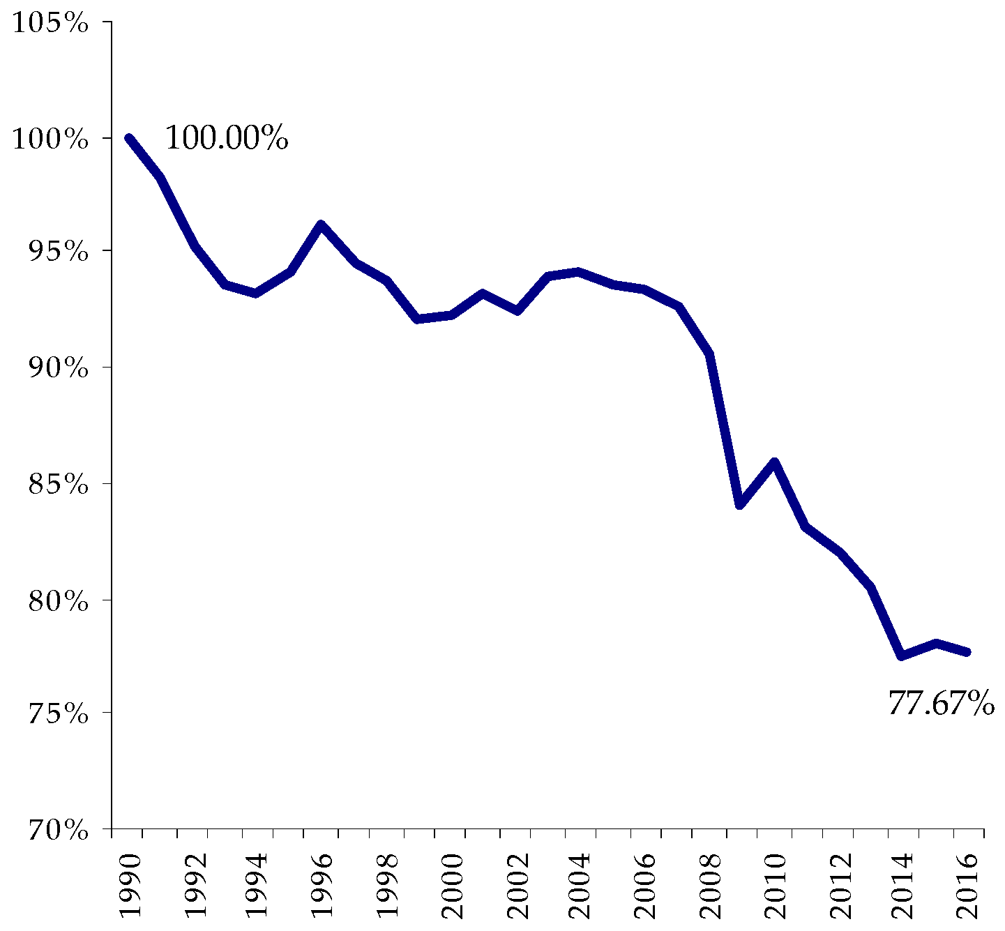
According to EUROSTAT [5] (p. 144), the main producers of GHG emissions in the European countries are: The supply of electricity, gas, steam and air conditioning; manufacturing; agriculture; forestry; and fishing. GHG emissions in 2016 in the EU reached 77.76% of the 1990 levels [6] (Figure 1). GHG emissions saw a downturn trend during the period 1990-1999, mainly due to structural changes (economic and political uncertainty and industrial activities which collapsed in the former communist countries), industrial modernization in Western countries and replacing coal with gas. Emissions increased in 1996, when a cold winter led to an increase in heating requirements [5], but the trend reversed in 1997. From 1998 to 2007 this trend decreased due to a growth in the use of low-carbon fuels, particularly renewable energy sources, offsetting an increase in primary energy consumption, as well as the use of lower-carbon footprints and the decline in livestock and nitrogenous fertilizer use in agriculture [7], (p. 2). The sharpest decline in energy consumption and pollutant emissions occurred between 2007 and 2009, due partly to the financial crisis (decrease in industrial production, demand and volume of transport) and also partly due to the switch from coal- to gas-fired electricity generation as a result of the adoption of the EU GHG Emission Trading Scheme (EU-ETS) [8], (p. 91). The decline observed between 2009 and 2012 can be attributed to larger shares of renewable energy sources in the fuel mix, the economic slowdown and an improvement in the energy intensity of the EU economy [9]. Between 2012 and 2014, the largest share of emissions reductions was achieved in the energy production sector (particularly in the case of electricity generation and heat production). In the last two years, a slight increase was noticeable, as a result of growing energy consumption from all sources, including fossil fuels, higher transport demands, increased economic growth and the increased consumption of gas used for heating in the residential sector [10].

Within the wealthy energy-growth-environment literature, several studies have explored the link between pollutant emissions as a dependent variable and various indicators (economic, social, geographic, demographic and technological) as explanatory variables. The present paper introduces a new explanatory variable in the analysis of the determinants of environmental degradation, namely, the economic complexity. Relevant studies on economic complexity, technological innovation and their relationship with energy consumption structure and pollution are discussed below.

In a general sense, economic complexity refers to a country’s productive structure, which leads to a specific structure of energy consumption and, as result, a specific effect on the environment. It is obvious that a country’s productive structure could influence GHG emissions while the complexity level of products could harm the environment by generating pollution, but it also embeds knowledge and capabilities, research and innovation, which can help to stimulate greener products and environmentally friendly technologies.

The increase in economic complexity is related to structural transformations in economies: Diversification from agriculture and extractive industries to more sophisticated products and services [11,12]. Several studies [13,14,15,16,17,18,19,20,21] in the last decade have dealt with the problem of quantifying a country’s productive structure.

According to the Center for International Development at Harvard University, the Economic Complexity Index (ECI) is an expression of the diversity and complexity of a country’s export basket [20]. The index is calculated for 128 countries, based on data from UN COMTRADE, the International Monetary Fund and World Development Indicators.

A higher value of ECI indicates improved (advanced) capabilities of a country in the production process [22,23]. The process of economic development could be explained as a process of learning how to produce and export more complex products [14,15], in turn requiring capabilities to develop new activities or products and attain a higher level of productivity.

Economic complexity is related to a country’s level of prosperity and there is a tight relationship between economic complexity and GDP per capita. Moreover, countries tend to move towards an income level which is compatible with their overall level of productive knowledge, meaning that their income tends to reflect their embedded knowledge [20]. The income level of countries tends to follow their productive structure [13,14,15]. According to the model developed by Hausmann and Hidalgo (2010) [24], the return to the accumulation of new capabilities increases exponentially with the number of capabilities already available in a country. The export shares of the most complex products could increase with income, while the export share of the less complex products could decrease with income. A more complex productive structure enables countries to engage in high productivity activities which lead to faster development [25].

Economic complexity is associated with income inequality: Increases in economic complexity tend to be accompanied by decreases in income inequality and a country’s productive structure may limit its range of income inequality [26].

As an accurate predictor of income per capita, [24] economic complexity may be used as explanatory variable when testing the validity of the Environmental Kuznetz Curve (EKC). An example is the study developed by Can and Gozgor (2017) [27] which noticed that the economic complexity is a significant indicator for suppressing the level of carbon emissions in France.

As an expression of a country’s innovative output, economic complexity is based on technological innovation and R&D activities in the economy, which generate not only more sophisticated and complex products, but may promote less polluting industrial technologies, efficiency in energy use and less environmental degradation.

The recent literature on energy research provides rich evidence confirming the role of technological innovation in reducing pollutant emissions and the transition to a lower-carbon economy.

The energy production sector is one of the main sources of pollutant emissions. Energy technology innovation could provide solutions which reduce emissions, augment energy resources and enhance the quality of energy services [28]. Energy technology innovation is a process ranging from R&D on new technologies to their diffusion, whose results are reflected in the market share and other aspects related to new technology diffusion [29]. Efforts to promote the deployment of new energy technologies can translate the results of R&D activities into changes in the energy system, with learning-by-doing being an important element of this deployment [30]. Effective policies for energy technology innovation can encourage energy projects and stimulate the development of energy users’ markets [31], as well as the transformation of energy consumption structure [32]. The efficiency of energy use can be improved through technological innovation as Miao et al. (2018) highlighted in the case of strategic emerging industries in China [33].

The gap between the patents in fossil fuel and renewable energy technology can be decreased through policies encouraging the market entrance of companies which are specialized in renewable technologies [34]. The integration degree between different technology classes of environmental patents is important to the environmental productivity performance of companies, as highlighted by Aldieri et al. (2017) in the case of water pollution. These authors proved that specialized environmental technology fields’ spillovers have a positive impact on firms’ productivity [35].

As an alternative in electricity production, the development of photovoltaic technologies and their participation in the renewable energy markets are driven by governments’ incentives (reduction in corporate income tax, subsidies to operators of renewable energy projects, financing lines) and energy efficiency policies. The leading countries involved in these technologies include the USA, China, Japan, Germany and South Korea [36,37].

Renewable energy expansion and the growth of the electric utility infrastructure have stimulated the interest in smart grid systems. A smart grid refers to an electricity network which can integrate, in an intelligent way, the actions of all connected users in order to deliver a sustainable, economical and secure electricity supply [38]. Based on digital technology, smart grids can improve the reliability, security, and efficiency of the electrical system through the delivery network to consumers and a growing number of distributed generation and storage resources [39].

As the chemical industry is one of the most emission-intensive sectors, R&D cooperation between chemical companies, universities and research institutes, as well as firms’ participation in industrial clusters could create knowledge spillover effects and sustainable innovation activities [40]. It is also important to shape policies supporting sustainability, eco-innovation and resource efficiency in this industry [41]. Eco-innovation can contribute to sustainable development [42], while environmentally friendly and socially responsible innovation fosters technological, institutional and organizational changes to the knowledge basis of existing production systems [43]. A number of external and internal factors is enabling eco-innovation and environmental change in companies: Technological, organizational, institutional, economical, market-related and societal [44]. The concept of eco-innovation is explored in the environmental literature in relation to the concept of sustainability transitions, which is defined as a long-term, multidimensional and radical transformation process leading to shifts in socio-technical systems towards more sustainable modes of production and consumption. Studies in this new field of research, which are mainly focused on energy and water supply, urban environment and transport, highlight how different green technologies could be combined in order to create new products, services, organizations and business models [45].

While the literature on the environment and innovation is focused on the contribution of innovation to reduce climate change impact, Su and Moaniba (2017) [46] used a reverse approach and discovered that a country’s propensity to innovate and patent climate change technologies is influenced by the levels of carbon dioxide and other GHG emissions.

External energy dependence in the European countries, increasing energy demand and the decline in conventional hydrocarbon reserves underline the call for other sources of energy (i.e., renewable and nuclear energy), although fossil fuels will remain the main source of available energy [47]. Within this context, carbon capture and storage (CCS) has been highlighted as a viable technology solution to reduce GHG emission and a mitigating strategy for climate change by Rodrigues et al. (2015) [47], Raza et al. (2019) [48], Mc Coy (2014) [49] and IEA (2011) [50]. An extension of carbon capture and storage technology is carbon capture and utilization (CCU) where the captured CO2 emission is also used as feedstock [51]. This is seen as a solution to improve the contradiction between economic development and environmental protection [52]. A detailed review of relevant papers on CCS and CCU technologies is provided by Yan and Zhang (2019) [53].

The energy consumption structure refers to the combination of different energy types (solid fuel, oil, gas, renewable, waste etc) in terms of final consumption. As a non-renewable energy source, fossil fuels are the most polluting component of the energy consumption structure. Due to their depletion and harmful effect on the environment, countries are forced to conceive energy policies from a global perspective on all energy sources and take into account the demand of the socio-economic system [54]. In order to achieve a significant reduction in their share in final consumption, energy considerations should be incorporated within the design phase of products [55]. The diversification of energy types, increasing the share of non-fossil energy and the development of renewable sources became priorities of energy policies in several countries [56,57,58,59]. Furthermore, hybrid renewable energy systems (combining several renewable energy sources) have gained the attention of business and industry in several countries [60,61], as well as micro grids composed of distributed energy resources [62,63].

Energy consumption structure, economic structure and energy efficiency exert a significant impact on pollutant emissions and can be considered as essential factors of low-carbon development [64,65,66]. Several methods have been developed in order to provide appropriate tools to analyse sectoral emission trends [67], simulate energy consumption and GHG emissions under different conditions [68], select economically feasible technologies [69] and models to optimize energy consumption structure [70] or improve energy structure in the industry [71].

An outstanding model of the global energy consumption structure was developed by Hu et al. (2018) in the form of an evolutionary tree, including 144 countries and regions. Developed countries have the most diverse energy consumption structures, while the location of countries in the evolutionary tree can provide a basis for improving these structures [72].

Energy consumption structure is connected with the economic structure. For example, the output of secondary industry has a higher effect on the energy consumption structure [73,74] than the tertiary industry [75].

Within the context of energy policies, energy consumption structure, as a technical term, is replaced with the concept of energy mix, which refers to a combination of various energy sources (coal, natural gas, nuclear, wind, solar power, biofuels) used to meet the energy needs of a country. The energy mix which leads to a reduction in carbon emission depends on the development level of the economy. Following the EKC hypothesis, Kim and Park (2018) [76] found out that the best energy policy mix for OECD countries involves a gradual decrease in their relative reliance on natural gas, nuclear power, biofuels and waste fuels in the short run, while solar and wind power energy sources can decrease carbon emissions in the long run as the economy continues to grow. The effect of energy mix on income depends on democracy level: Less democratic countries tend to become more dependent on oil and natural gas with their own development while more democratic countries tend to move away from oil and geothermal sources and encourage the development of renewable energy sources [77].

Considering the above, it can be noted that the relationship between economic complexity and GHG emissions has not been analysed to date in the relevant literature, except for the aforementioned work of Can and Gozgor (2017) [27] which tests the validity of the EKC hypothesis in the French economy. The aim of the paper is to examine the long-term relationship between economic complexity, energy consumption structure and GHG emissions within a panel of 25 European Union countries. In addition, the analysis is carried out within two subpanels of European economies, in order to reveal country features which could affect the intensity of the relationship between economic complexity, energy consumption structure and GHG emissions.

The first contribution to the literature of this empirical study is that it analyses the long-run dynamics of economic complexity, energy consumption structure and GHG emissions in a panel data approach. The second contribution is related to the fact that a large part of the energy-growth- environment literature, which examines this relationship by employing panel data methods, assumes that panel time-series data are homogeneous and cross-sectionally independent which could cause possible inference and forecasting errors. To fill this gap, our study employs heterogeneous panel estimation techniques with cross-sectional dependence.

To the best of our knowledge, the present study is the first to examine the relationship between the ECI, energy consumption structure and GHG emissions in a panel data model.

The organizational structure of the paper is as follows: Section 2 provides the empirical model for this study, data sources and descriptive statistics; Section 3 presents the econometric modelling outcome; Section 4 discusses the results; and Section 5 concludes the paper with a summary of the main findings and policy implications.

2. Materials and Methods

2.1. Model and Data

According to existing studies [66,78,79], the sectoral structure of the economy and the composition of energy consumption (solid fuels, oil, gas, and renewable energy), as well as the economic complexity [27] influence the level of pollutant emissions. The economic complexity was chosen as the primary explanatory variable because it is considered an accurate predictor of economic growth and expression of a skill-based, knowledge-based and sophisticated production [22], which was not included before in a panel analysis of environmental impact. The reason for including energy consumption structure as the second explanatory variable is related to the fact that the increase of fossil share in energy consumption influences the carbon emissions and environment deterioration [66,78,79] and improvement of the energy consumption structure has a great impact on greening the economy and transitioning to a lower carbon-stage.

In order to explore the relationship between economic complexity, energy consumption structure and GHG emissions in the European Union countries, the panel data methodology is utilized due to its ability to control heterogeneity and serial correlation [80]. Thus, the paper proposes a model including three variables Equation (1):

$$GH{G}_{it}=f(EC{I}_{it},ECS{P}_{it}),$$

(1)

where: $GH{G}_{it}$ denotes the GHG emissions (thousand tones), $ECS{P}_{it}$ is the energy consumption share generating air pollution (GHG emissions), $EC{I}_{it}$ is the Economic Complexity Index, i denotes the country and t the time.

The Economic Complexity Index (ECI) is the expression of a country productive structure by combining information on the diversity (number of products it exports) Equation (2) and the ubiquity (the number of countries that export that product) Equation (3) [15].

A country is able to manufacture a product if has all the available capabilities, hence it is connected with other countries to produce it, resulting in a network of interconnected countries. A product can be exported by several countries and a country exports products made by using capabilities of other countries, resulting bipartite networks in which countries are connected to the products they export. Mathematically, this network is represented using the adjacency matrix ($M_{cp}$). $M_{cp}$ = 1 when the country c is a significant exporter of the product p and 0 otherwise.

$$Diversity=k_{c,0}={\displaystyle \sum _p{M}_{cp}},$$

(2)

$$Ubiquity=k_{p,0}={\displaystyle \sum _c{M}_{cp}},$$

(3)

where: $k_{c,0}$ represent, respectively, the levels of diversification of a country and $k_{p,0}$ the ubiquity of a product.

The Revealed Comparative Advantage ($RC{A}_{cp}$) Equation (4) of a country c in product p is:

$$RC{A}_{cp}=\frac{X_{cp}/{\displaystyle \sum {}_{p^{\prime }}{X}_{c{p}^{\prime }}}}{{\displaystyle \sum {}_{c^{\prime }}{X}_{c^{\prime }p}/{\displaystyle \sum {}_{c^{\prime }{p}^{\prime }}{X}_{c^{\prime }{p}^{\prime }}}}},$$

(4)

where: $X_{cp}$ is the total export of country c in product p. A value of RCA higher than 1, indicates a comparative advantage of the country in a product.

The link between $M_{cp}$ and $RC{A}_{cp}$ Equations (5) and (6) is shown below:

$$M_{cp}=1\mathrm{if}RC{A}_{cp}\ge 1,$$

(5)

$$M_{cp}=0\mathrm{if}RC{A}_{cp}<1.$$

(6)

Countries exporting similar products can be connected defining a new matrix, weighted by the inverse of the ubiquity of a product and normalized by the diversity of a country ${\tilde{M}}_{c{c}^{\prime }}$ Equation (7):

$${\tilde{M}}_{c{c}^{\prime }}=\frac{1}{k_{c,0}}={\displaystyle \sum \frac{M_{cp}{M}_{c^{\prime }p}}{k_{p,0}}}.$$

(7)

The Economic Complexity Index (ECI) Equation (8) is defined as:

$$EC{I}_c=\frac{K_c-(K)}{std(K)},$$

(8)

where: $K_c$ is the eigenvector of ${\tilde{M}}_{c{c}^{\prime }}$ associated with the second largest eigenvalue [16].

Taking into consideration that the share of renewable energy consumption (FREC) in the final energy consumption (FEC) doesn’t harm the environment, the difference to the total final energy consumption (FEC-FREC) will generate air pollution (GHG emissions). Thus, we can express the share of final energy consumption generating pollution (ECSP) Equation (9), as follows:

$$ECS{P}_{it}=\frac{FE{C}_{it}-FRE{C}_{it}}{FE{C}_{it}}.$$

(9)

ECSP reveals the energy consumption structure. A higher level of ECSP indicates a high share of non-renewable (fossil) energy consumption in the total final consumption. The values of final energy consumption and final renewable energy consumption were extracted from EUROSTAT database, Energy Balances, May 2018 Edition [81].

The EUROSTAT database was also the source of data on GHG emissions. The values of ECI were collected from the Centre of International Development at Harvard University [82]. Data used in the study are regarding the period of 1995–2016.

In order to reduce data fluctuation and avoid panel heteroskedasticity, the variable GHG is converted in natural logarithms, expressed as lnGHG.

Equation (1) is re-written Equation (10) as follows:

$$\ln GH{G}_{it}={\beta }_1\cdot EC{I}_{it}+{\beta }_2\cdot ECS{P}_{it}+{\mu }_{it}$$

(10)

where: ${\beta }_1$ and ${\beta }_2$ are elasticities of GHG as regards to ECI and ECSP, respectively ${\mu }_{it}$ is the error.

We use a panel of 25 European Union countries: Austria, Belgium, Bulgaria, Germany, Denmark, Spain, Estonia, Finland, Hungary, Ireland, Italy, United Kingdom, Greece, Poland, Portugal, Slovak Republic, Slovenia, Romania and Sweden. 3 Member States (Cyprus, Malta and Luxembourg) were excluded due to the lack of ECI series.

In order to capture disparities among the EU countries in their influence of economic complexity on GHG emissions, we divided the 25 EU panel members into groups (subpanels) according to the average values of ECI for the period of 1995–2016. The first subpanel consists of 15 EU countries (Sweden, Belgium, the Czech Republic, Germany, Austria, Finland, United Kingdom, France, Slovenia, Italy, Slovak Republic, Denmark, Netherlands, Ireland, Hungary) with average values of ECI between 1.14 (Netherlands) and 2.19 (Germany). The second subpanel includes 10 EU countries (Poland, Spain, Croatia, Estonia, Romania, Portugal, Lithuania, Latvia, Greece, Bulgaria) with average values of ECI between 0.13 (Greece) and 0.99 (Poland). The descriptive statistics of all variables are displayed in

Table 1. Descriptive statistics for all variables.

Panel	Variable	Mean	Median	Max.	Min.	St.dev.	Skewness	Kurtosis
EU panel	lnGHG	11.53999	11.20643	13.96116	9.260405	1.186123	0.163749	2.230939
	ECI	1.202207	1.285350	2.474000	−0.013500	0.554185	−0.095583	2.179843
	ECSP	0.908034	0.926871	0.996845	0.728461	0.064875	−0.616996	2.507284
first panel	lnGHG	11.82719	11.35518	13.96116	9.725573	1.101350	0.350489	2.160422
	ECI	1.578725	1.538700	2.474000	0.772900	0.323709	0.369924	2.806533
	ECSP	0.931705	0.945898	0.996845	0.777919	0.0550467	−0.900467	2.871039
second panel	lnGHG	11.10917	11.15328	13.03083	9.270405	1.180629	0.157199	1.772303
	ECI	0.637431	0.641150	1.208800	−0.013500	0.280068	−0.179867	2.380175
	ECSP	0.872528	0.865493	0.994414	0.728461	0.062341	−0.334846	2.307824

.

2.2. Econometric Specifications

Due to the interdependence of European economies as a result of their integration in the EU internal market and of EU common policies, a cross-sectional dependence across examined panels could exist. Additionally, regarding heterogeneity, when dealing with panel data methodologies, it is assumed that the variations between cross-sectional units are captured by fixed constants. However, some individual variability of the cross-sections may exist (due to differences in economic and productive structure, energy system, pollutant emissions) and if it is not taken into consideration, it may bias the results and cause incorrect inference. Therefore, the causality relationship between the variables under study will be explored by using heterogeneous panel causality and estimation techniques developed by Dumitrescu and Hurlin (2012) [83].

Thus, in our analysis: (i) Cross-sectional dependence will be examined, (ii) stability of data series will be tested with panel unit root test, (iii) long-term relationship between variables will be investigated through the panel cointegration method, (iv) if the cointegration between variables is confirmed, the fully modified ordinary least square (FMOLS) and dynamic ordinary least square (DOLS) will be used to estimate the long-term elasticity between the dependent and the independent variables, and (v) causality relationship between variables will be examined with the Dumitrescu and Hurlin (2012) test [83].

Testing the cross-sectional dependence across panels was used by Dogan and Aslan (2017) [84] when exploring the relationship between carbon emissions, energy consumption and tourism and by Sun et al. (2018) [68] when analysing the link between energy consumption, economic growth, urbanization and carbon emissions. The panel cointegration method is largely employed in empirical studies investigating the link between economic growth and renewable energy [85,86,87,88,89,90,91,92,93,94,95,96,97] and also, in exploring the relationship between carbon emissions, energy consumption and economic development [98]. The estimation of long-run parameters with fully modified ordinary least square (FMOLS) and dynamic ordinary least square (DOLS) methods is also used in almost all above mentioned studies [85,86,87,88,89,90,91,92,93,94,95,96,97,98], as well as by Dogan and Aslan (2017) [84].

2.2.1. Cross-section Dependence in Panel Data

Cross-section dependence in our panel data will be examined by using the following tests: Breusch-Pagan LM (1980) [99], Pesaran scaled LM and Pesaran CD (2004) [100].

Based on Pesaran (2004) [100] considerations, in a panel data model Equation (11):

$$y_{it}={\beta }_{it}\cdot x_{it}+u_{it},$$

(11)

$x_{it}$ is k-dimensional column vector of regressors and ${\beta }_i$ are the corresponding cross-section specific vectors of parameters to be estimated, i = 1, 2, …, N (the number of cross-sections) and t = 1, 2, …, T (time). Under the null hypothesis of no cross-section dependence Equation (12), the correlation of disturbances between different cross-sections is zero:

$$H_0:{\rho }_{ij}=corr(u_{it},u_{jt})=0,\mathrm{for}i\ne j.$$

(12)

While the alternative hypothesis Equation (13) states:

$$H_1:\mathrm{exists}i\ne j\mathrm{making}{\rho }_{ij}=corr(u_{it},u_{jt})\ne 0.$$

(13)

According to Pesaran (2004) [100], in balanced panels ${\rho }_{ij}$ is the product-moment correlation coefficient of the residuals Equation (14):

$${\widehat{\rho }}_{ij}=\frac{{\displaystyle \sum _{t\in i,j}^{T_{kj}}{\widehat{u}}_{it}{\widehat{u}}_{jt}}}{{\left({\displaystyle \sum _{t\in i,j}^{T_{jk}}{\widehat{u}}_{it}^2}\right)}^{1/2}{\left({\displaystyle \sum _{t\in i,j}^{T_{jk}}{\widehat{u}}_{jt}^2}\right)}^{1/2}}.$$

(14)

The notation $t\in i,j$ is used to indicate that we sum over the subset of $T_{ij}$ observations common to i and j to obtain the pairwise mean ${\tilde{u}}_i$ Equation (15), as below:

$${\tilde{u}}_i=\frac{{\displaystyle \sum _{t\in i,j}^{}{\widehat{u}}_{it}}}{T_{ij}}.$$

(15)

The pairwise mean is used to adjust the residuals in pairwise subsets which are not necessarily mean zero.

In the unbalanced panels, Pesaran (2004) [100] proposes the centred correlation coefficient Equation (16) as follows:

$${\widehat{\rho }}_{ij}=\frac{{\displaystyle \sum _{t\in i,j}^{T_{kj}}({\widehat{u}}_{it}-{\tilde{u}}_i)({\widehat{u}}_{jt}-{\tilde{u}}_i)}}{\sqrt{{\displaystyle \sum _{t\in i,j}^{T_{kj}}{({\widehat{u}}_{it}-{\tilde{u}}_i)}^2}}\sqrt{{\displaystyle \sum _{t\in i,j}^{Tkj}{({\widehat{u}}_{jt}-{\tilde{u}}_i)}^2}}}.$$

(16)

According to the Breusch-Pagan (1980) [46] Lagrange Multiplier (LM) test, the LM statistic dependence under the null hypothesis Equation (17) is given by:

$$LM={\displaystyle \sum _{i=1}^{N-1}{\displaystyle \sum _{j=i+1}^N{T}_{ij}{\widehat{\rho }}_{ij}^2\to {\chi }_{\frac{N(N-1)}{2}}^2}},$$

(17)

where: ${\widehat{\rho }}_{ij}$ denotes correlation coefficients obtained from the residuals and ${\chi }^2$ is the asymptotic distribution obtained for N fixed and $T_{ij}\to \infty$ for all $(i,j)$ under a normality assumption of errors.

Recognizing that the Breusch-Pagan test is not appropriate for large N, Pesaran (2004) [100] proposed first a standardized version of LM statistic, the scaled LM Equation (18):

$$L{M}_s=\sqrt{\frac{1}{N(N-1)}}{\displaystyle \sum _{i=1}^N{\displaystyle \sum _{j=i+1}^N\left(T_{ij}{\widehat{\rho }}_{ij}^2-1\right)}}\to N(0,1),$$

(18)

where: first $T_{ij}\to \infty$ and then $N\to \infty$, for an asymptotical normal distribution.

In order to address the shortcomings of the LM test related to the fact that $(T_{ij}{\widehat{\rho }}_{ij}^2-1)$ is not centered at zero for finite $T_{ij}$ and the results are distorted for large N, Pesaran (2004) [100] proposed an alternative based on the average of the pairwise correlation coefficients Equation (19):

$$CD=\sqrt{\frac{2}{N(N-1)}}\left({\displaystyle \sum _{i=1}^{N-1}{\displaystyle \sum _{j=i+1}^N{T}_{ij}{\widehat{\rho }}_{ij}\to N(0,1)}}\right),$$

(19)

for $T_{ij}\to \infty$ and $N\to \infty$ in any order for an asymptotical normal distribution.

When applying these tests, the values of Prob under 0.05 will indicate the rejection of null hypothesis of no cross-section dependence.

2.2.2. Unit Root Tests in Panel Data

In the panel data literature there are some models commonly used for testing stationarity of variables in panel analysis, introduced by Levin, Lin and Chu (LLC) (2002) [101], Im, Pesaran and Shin (IPS) (2003) [102], Madalla and Wu (1999) [103], even in the presence of cross-sectional dependence [104].

When testing stationarity of panel time series, we consider an autoregressive AR (1) process across sections in panel data Equation (20), as follows:

$$y_{it}={\rho }_i{y}_{it-1}+x_{it}{\delta }_i+{\epsilon }_{it},$$

(20)

where: i = 1, 2, …, N denotes the cross-sections, t = 1, 2, …, $T_i$ denotes the periods of time, $x_{it}$ represent the exogenous variables (including any fixed effects or individual trends), ${\rho }_i^{}$ are the autoregressive coefficients and ${\epsilon }_{it}$ represent the errors, assumed to be mutually independent idiosyncratic disturbance. When $|{\rho }_i|=1$, then $y_i$ contains a unit root.

There are two assumptions regarding the ${\rho }_i^{}$. First, we can assume that ${\rho }_i=\rho$ for all i, meaning that the parameters are common across all cross-sections. The Levin, Lin and Chu (LLC) (2002) [101] developed a panel unit root test using this assumption. The alternative assumption is that the parameters can vary across cross-sections. An example of a test using it is developed by Im, Pesaran and Shin (IPS) (2003) [102].

Levin, Lin, and Chu (LLC) [101] test assumes that there is a common and identical unit root process across cross-sections. The following specification Equation (21) is considered:

$$\Delta y_{it}=\alpha \cdot y_{it-1}+{\displaystyle \sum _{j=1}^{p_i}{\beta }_{ij}}\cdot \Delta y_{it-j}+{X^{\prime }}_{it}\cdot \delta +{\epsilon }_{it},$$

(21)

where: $\alpha =\rho -1$ is common for all cross-sections and the lag order for difference terms $p_i$ may vary across cross-sections.

The null hypothesis of a unit root Equation (22) is given by:

$$H_0:\alpha =0,$$

(22)

and the alternative hypothesis (absence of a unit root) Equation (23) is written as follows:

$$H_1:\alpha <0.$$

(23)

The Im, Pesaran, and Shin (IPS) (2003) [102] test allows for individual unit root processes, so ${\rho }_i$ may vary across cross-sections. Within this test a separate Equation regression (21) is conducted in each cross-section.

The null hypothesis Equation (24) is written as follows:

$$H_0:\alpha =0\mathrm{for}\mathrm{all}i.$$

(24)

The alternative hypothesis (of stationarity) Equation (25) is given by:

$$H_1:{\alpha }_i=0\mathrm{for}\mathrm{i}=1,2,\dots ,N_1;{\alpha }_i<0\mathrm{for}\mathrm{i}=\mathrm{N}+1,\mathrm{N}+2,\dots ,\mathrm{N}.$$

(25)

2.2.3. Panel Cointegration Test

It is well known that many economic time series are not stationary, but a stationary process could be identified in their first difference series. Engel and Granger (1987) [105] noted that a linear combination of two or more such series may be stationary, in which case we say that they are cointegrated and the linear combination defines the cointegration equation with cointegrating vectors of weights, reflecting the long-run relationship between the variables.

Given the results of the panel unit root tests the next decision is regarding the estimation of regression Equation (3). If the variables are not stationary at their level value, but integrated of the first order, the cointegration relation can be examined.

We use the panel cointegration test developed by Pedroni [106,107]. Within this test, seven different test statistics are run: Four of them consist of in-group statistics (panel-v, panel-$\rho$, semiparametric panel-t and parametric panel-t) and other three consist of intergroup (group-$\rho$ statistics, semiparametric group-t and parametric group-t) statistics. The interpretation of test results is as follows. The values of Prob for each statistic are compared with the selected significance level (1% or 5%). If the number of statistics with values of Prob below the significance level is at least 4, the null hypothesis (of no cointegration for all i) is rejected meaning that there is a long-term relationship between the variables.

2.2.4. Estimation of Long-Run Parameters

The cointegration coefficients can be estimated through the panel fully modified ordinary least squares (FMOLS) and the panel dynamic ordinary least squares (DOLS) methods developed by Pedroni [108,109].

The panel FMOLS equation Equations (26) and (27) can be written as follows:

$$y_{it}={\alpha }_{it}+{\delta }_{it}t+\beta x_{it}+{\mu }_{it},$$

(26)

$$x_{it}=x_{it-1}+e_i,$$

(27)

where: $y_{it}$ is the dependent variable and $x_{it}$ is the independent variable, ${\alpha }_{it}$ denotes the constant effects, $\beta$ is the long-term cointegration coefficient/vector that should be estimated if we assume that there is no dependence between panel sections.

The panel FMOLS estimator Equation (28) is specified as below:

$${\widehat{\beta }}_{FM}^{*}=n^{-1}{\displaystyle \sum _{i=1}^n{\widehat{\beta }}_{FM,i}^{*}},$$

(28)

where: ${\widehat{\beta }}_{FM}^{*}$ is the FMOLS estimation result for a cross-section that forms each i-th section.

The cointegration coefficient for the overall panel is estimated with the average of FMOLS coefficients in the cross-sections.

T-statistic for the panel cointegration coefficient ($t_{{\widehat{\beta }}_{FM}^{*}}^{*}$) Equation (29) is calculated as below:

$$t_{{\widehat{\beta }}_{FM}^{*}}^{*}=n^{-1}{\displaystyle \sum _{i=1}^n{t}_{{\widehat{\beta }}_{FM,i}^{*}}}.$$

(29)

The panel DOLS method introduced by Pedroni [55] is specified Equation (30) as follows:

$$y_{it}={\alpha }_i+{\beta }_i{x}_{it}+{\displaystyle \sum _{k=-K_i}^{K_i}{\gamma }_{it}}\Delta x_{it-K}+{\epsilon }_{it}.$$

(30)

This equation is estimated for each cross-section of the panel and then the cointegration coefficient for the overall panel is calculated as the average of the DOLS coefficients for each section.

The panel DOLS estimator Equation (31) is calculated as below:

$${\widehat{\beta }}_D^{*}=n^{-1}{\displaystyle \sum _{i=1}^n{\widehat{\beta }}_{D,i}^{*}},$$

(31)

and the t-statistic for the panel cointegration coefficient Equation (32):

$$t_{{\widehat{\beta }}_D^{*}}^{*}=n^{-1}{\displaystyle \sum _{i=1}^n{t}_{{\widehat{\beta }}_{D,i}^{*}}}.$$

(32)

2.2.5. Panel Causality Test

We intend to find the direction of causality between the variables by using the test developed by Dumitrescu and Hurlin (2012) [83].

In this test the null hypothesis (of no causality from x to y) Equation (33) is defined as follows:

$$H_0:{\beta }_i=0\mathrm{for}\forall i=1,\dots ,n;{\beta }_i=({\beta }_i^{(1)},{\beta }_i^{(2)},\dots ,{\beta }_i^{(k)}).$$

(33)

Under the alternative hypothesis Equation (34), we assume that there are $n_1$ < n individual processes with no causality from x to y:

$$H_1:{\beta }_i=0\mathrm{for}\forall i=1,\dots ,n_1;{\beta }_i\ne 0\mathrm{for}\forall i=n_1,n_1+1,n_1+2,\dots ,n,$$

(34)

where: $n_1$ is unknown and $0\le \frac{n_1}{n}$ < 1. If $n_1=n$, then it is no causality for any sections in the panel.

If $n_1=0$, there is causality for all sections in the panel. If $n_1>0$, the causality relationship is heterogeneous, meaning that the regression model and causality relations are different from one section to another. In this context, Dumitrescu and Hurlin (2012) [56] proposed to use the average Wald statistic in association with the test of non-causality hypothesis for $i=1,\dots ,n$.

In order to reveal the causality relationship in each section of the panel, individual Wald statistics for each section are computed and then the Wald statistic for the overall panel is obtained as the average of the individual Wald statistics Equation (35):

$$W_{n,T}=\frac{1}{n}{\displaystyle \sum _{i=1}^n{W}_{i,T}}.$$

(35)

Each individual Wald statistic converges to a chi-squared distribution with K degrees of freedom under the null hypothesis of non-causality Equation (36):

$$W_{i,T}\stackrel{d}{\to }{\chi }^2(K),\forall i=1,\dots ,n;T\to \infty .$$

(36)

When T tends to infinity, the individual Wald statistics are identically distributed, under the assumption that individual residuals ${\epsilon }_i$ are independently distributed across groups.

When $T\to \infty$ first and then $n\to \infty$, meaning that $T<n$, the standardized test under this condition Equation (37) is shown below:

$$Z_{n,T}=\sqrt{\frac{n}{2K}}\left(W_{n,T}-k\right)\to n\left(0,1\right).$$

(37)

When Z-statistic is higher than the corresponding critical value for a given level of risk, the homogenous non-causality hypothesis is rejected.

3. Results

3.1. Cross-Section Dependence Test

Table 2. Cross-sectional dependence test results.

Test	EU Panel		First Subpanel		Second Subpanel
	Statistic	Prob	Statistic	Prob	Statistic	Prob
Breusch-Pagan LM	1365.742	0.000	474.614	0.000	233.799	0.000
Pesaran scaled LM	43.508	0.000	25.505	0.000	19.901	0.000
Pesaran CD	16.713	0.000	9.611	0.000	5.83	0.000

presents the results of cross-sectional dependence examination for all 3 types of tests (Breusch-Pagan LM, Pesaran scaled LM and Pesaran CD) in the EU panel and the two subpanels.

We notice from the Table 2 that for all tests, the value of Prob is 0.000, indicating the rejection of the null hypothesis at 1% significance level in all panels and revealing the presence of cross-sectional dependence.

3.2. Panel Unit Root Test

As described above, because of the existence of cross-sectional dependence, in this section, the stationarity of lnGHG, ECI and ECSP will be inspected in all panels.

Due to the cross-sectional dependence identified above, we run the LLC and IPS test for all variables in all panels.

Table 3. Panel unit root test results.

Panel	Variable		LLC Test		IPS Test
			t-Statistic	Prob	t-Statistic	Prob
EU panel	lnGHG	level	0.86198	0.8195	2.03363	0.9790
		first difference	−6.42057	0.0000	−9.35709	0.0000
	ECI	level	−1.97219	0.0243	0.89888	0.8156
		first difference	−9.25390	0.0000	−13.9851	0.0000
	ECSP	level	2.11793	0.9829	3.85146	0.9999
		first difference	−4.55741	0.0000	−7.11993	0.0000
first subpanel	lnGHG	level	2.30866	0.9895	4.40923	1.0000
		first difference	−2.28777	0.0111	−7.23937	0.0000
	ECI	level	−1.82967	0.0336	0.56182	0.7129
		first difference	−4.28416	0.0000	−10.8874	0.0000
	ECSP	level	3.35665	0.9996	6.24111	1.0000
		first difference	−3.46770	0.0003	−5.50786	0.0000
second subpanel	lnGHG	level	−1.87786	0.0302	−2.18474	0.0145
		first difference	−6.56538	0.0000	−5.92847	0.0000
	ECI	level	−0.79200	0.2142	0.73316	0.7683
		first difference	−9.11976	0.0000	−8.77809	0.0000
	ECSP	level	−1.48278	0.0691	−1.55408	0.0601
		first difference	−2.96510	0.0015	−4.51188	0.0000

displays the results of LLC and IPS test in all panels. We notice that the series of variables at level value are not stationary, except ECI within the EU panel and first subpanel (LLC test) and lnGHG in the second subpanel (LLC test and IPS test). All variables are stationary in their first difference series, that is, they are integrated at the first order.

3.3. Panel Cointegration Test

Table 4. Cointegration results (Pedroni test).

Test	EU Panel		First Subpanel		Second Subpanel
	Statistic	Prob.	Statistic	Prob.	Statistic	Prob.
Panel v-statistic	−1.628482	0.9483	0.300148	0.3820	−2.123516	0.9831
Panel rho-statistic	−1.385798	0.0829	−2.033569	0.0210	−0.204069	0.4191
Panel PP-statistic	−6.757617	0.0000	−7.359821	0.0000	−2.781790	0.0027
Panel ADF-statistic	−6.844862	0.0000	−7.809627	0.0000	−2.473985	0.0067
Panel rho-statistic	0.27580	0.6085	−0.587692	0.2784	1.55345	0.8760
Panel PP-statistic	−7.321569	0.0000	−7.603096	0.0000	−2.264564	0.0118
Panel ADF-statistic	−7.266844	0.0000	−7.799332	0.0000	−1.937699	0.0263

Note: Newey-West Bandwidth selection with Bartlett Kernel is used, under the assumption of deterministic intercept and trend and selection of Schwarz Info criterion.

exhibits the panel cointegration results. In the EU panel we have 4 out of 7 statistics with their corresponding value of Prob. under 0.5, in the first subpanel there are 5 and in the second subpanel there are 4. This indicates a cointegration relationship between lnGHG, ECI and ECSP in all three panels.

3.4. Estimation of Long-Run Coefficients

The FMOLS and DMOLS techniques are used to estimate elasticities of lnGHG with respect to ECI and ECSP. The estimation results of FMOLS and DMOLS equations are shown in

Table 5. Estimation of long-run coefficients

EU Panel
Variable	Panel FMOLS			Panel DMOLS
	Coefficient	t-Statistic	Prob.	Coefficient	t-Statistic	Prob.
ECI	0.151272	3.287310	0.0011	0.085603	2.478900	0.0136
ECSP	3.364968	10.06761	0.0000	3.379910	14.23777	0.0000
R-squared	0.998093			0.998754
First Subpanel
Variable	Panel FMOLS			Panel DMOLS
	Coefficient	t-Statistic	Prob.	Coefficient	t-Statistic	Prob.
ECI	0.109915	2.050873	0.0412	0.076564	2.244909	0.0257
ECSP	2.943705	7.299848	0.0000	2.974979	12.68415	0.0000
R-squared	0.998528			0.998894
Second Subpanel
Variable	Panel FMOLS			Panel DMOLS
	Coefficient	t-Statistic	Prob.	Coefficient	t-Statistic	Prob.
ECI	0.186747	2.418037	0.0166	0.155283	2.096166	0.0379
ECSP	3.763557	6.922499	0.0000	3.768395	6.660341	0.0000
R-squared	0.997455			0.998323

Notes: (1) Selected options for FMOLS equations estimation: Linear trend, pooled panel method; (2) Selected options for DMOLS equations estimation: Linear trend, Schwarz lag method, weighted pooled panel method.

.

The estimation of FMOLS and DMOLS equations indicate that ECI has a validated statistical influence on lnGHG, for a significance threshold of 5%, in the UE panel and both subpanels. The influence is also validated for the influence of ECSP on lnGHG at a significance level of 1% in all panels.

In the UE panel, the long-run elasticity of GHG emissions with respect to energy consumption structure is 3.36, indicating a positive association between the two variables and, as expected, the increase of the share of activities generating air pollution has, as a consequence, a greater quantity of GHG emissions. According to the FMOLS equation estimation, the GHG emission will increase with 0.15% when ECI increases with 1%, respectively with 3.36% when the share of energy consumption for pollutant activities will increase with one percent. In the DMOLS equation estimation, the influence of ECI on lnGHG is lower than in the FMOLS estimation and the influence of ECSP is similar.

In the first subpanel of EU countries with a high level of products complexity, the elasticity of lnGHG related to ECI is lower than in the EU panel in both estimations (FMOLS and DMOLS). In the FMOLS estimation, when ECI increases with 1%, GHG emissions (as ln) will increase with 0.1% and the increase of ECSP with 1% will generate an increase in lnGHG emissions of 2.94%.

In the second subpanel of EU countries with lower economic complexity of products, the elasticity of ECI related to lnGHG is the highest of all panels (0.18), as well as ECSP (3.76), and likewise in the FMOLS specification, as well as in the DOLS estimation (0.15 for ECI; and 3.76 for ECSP). A 1% increase of ECI will generate an increase of lnGHG of 0.18% and a 1% increase of ECSP will lead to an increase of lnGHG of 3.76%, according to the estimated FMOLS coefficients.

3.5. Panel Causality Test

We used the Dumitrescu-Hurlin test to check the heterogeneous panel causality, but the results are not conclusive for all panels (

Table 6. Panel causality test.

Causality	EU Level	First Subpanel	Second Subpanel
	Prob. of Z-bar Stat
$\Delta ECI\to \Delta \ln GHG$	0.56 (1)	0.21(4)	0.87(1)
$\Delta ECSP\to \Delta \ln GHG$	0.00 (1 to 2)	0.00 (1 to 4)	0.07(1)

Note: In brackets: The number of lags.

).

A validated causality from the ECSP variation to lnGHG variation in the EU panel is identified and also in the first subpanel of countries (with high economic complexity of their products), for a number of maxim 2 lags in the EU panel and for 4 maxim lags in the first subpanel. The causality from economic complexity to greenhouse gas emissions could not be demonstrated.

4. Discussion

4.1. Dynamics of Energy Consumption Structure and GHG Emissions in the EU Countries

There is a decreasing trend in the share of non-renewable energy in the total final consumption (ECSP) in all 25 EU countries. This trend is obvious in the first subpanel of countries (Figure 2a) while in the second subpanel (with lower economic complexity) there are contrasting developments: In Bulgaria and Romania the pollutant activities increased from 1995 to 2016, in Spain and Portugal the extent of oscillations is of 2 to 6 percentage points and an increasing trend in the last years is shown in Croatia, Lithuania, Spain and Portugal (Figure 2b).

The annual average rate of ECSP decrease in the first group of countries is higher than in the second subpanel, even if the share of non-renewable energies in the total final consumption (ECSP) is higher than in the second group of countries; the countries from the second subpanel have lower shares of non-renewable energies but the annual average rate of reduction is only 0.147% compared to 0.2035% in the countries of the first subpanel (Figure 3a,b).

All the countries from the first subpanel registered a noticeable decreasing trend of their share of non-renewable energies in total final energy consumption, as exhibited in Figure 3a. The highest reducing speeds are registered in Sweden, Austria, Slovenia, Slovak Republic and Belgium and low performance in reducing pollutant activities can be noticed in the Czech Republic and Ireland.

In the second group of countries (see Figure 3b), Romania and Bulgaria have a different evolution of the share of fossil energy consumption; the average annual growth of the pollutant activities is 0.22% in Bulgaria and 0.14% in Romania. In the rest of countries, Greece and Poland are standing out with high speeds of ECSP decrease, while low performers are Estonia and Croatia, as well as Portugal with a decrease rate close to zero.

Countries with higher performance in products complexity are countries with a high share of non-renewable energy consumption, tempted to invest in less pollutant industrial technologies and renewable energy sources generating a higher speed of reducing the pollutant activities. Countries with lower performance in their product complexity are experiencing a lower rate of reducing their share of fossil energy consumption.

Among the countries from the first subpanel, Austria registered the deepest decrease of GHG emissions, from 1995, but in 2016 the emissions are higher when compared to 2015. An increasing trend is obvious in several countries in the last years: The United Kingdom, Italy, Sweden, Slovak Republic, Slovenia and Hungary. After the decreasing dynamics in the period of 1995–2014, Finland, Germany and Denmark have a stable evolution in the last years (Figure 4a).

There is a slight decreasing trend of the lnGHG among the countries included in the second subpanel, from 1995 to 2016, but Romania and Estonia registered values above the 1995 level. A slight increasing trend can be identified in the last years in Portugal, Romania, Spain and Latvia (Figure 4b).

The average annual decrease rate of GHG emissions is higher in the first subpanel (0.07%) as in the second subpanel (0.04%). The best performers of the GHG emissions decrease in the first subpanel are: Austria, Netherland, Belgium and Denmark. Average annual growth rates of GHG emissions are registered by the United Kingdom and Italy (Figure 5a). In the second subpanel, Greece stands out with the highest average annual decrease rate of GHG, followed by Poland and Portugal. Romania and Estonia experienced positive rates of GHG variation, in other words, annual increases of GHG (Figure 5b).

4.2. Country Features Affecting the Intensity of the Relationship Between Economic Complexity, Energy Consumption Structure and GHG Emissions

As it can be noticed from the last section, in all panels, the growth of the share of fossil energy in the total final energy consumption (ECSP) and of economic complexity (ECI) has led to increased greenhouse gas emission (lnGHG). The values of elasticity coefficients are statistically significant and higher in the second subpanel of countries with lower economic complexity than in the first subpanel and at the EU level. How can we explain this difference between the two groups of EU countries regarding the impact of economic complexity and energy consumption structure on GHG emissions? We discuss below country features that could affect this impact.

4.2.1. The Subpanel of Countries with Higher Economic Complexity

The increase in income in the last decades in these countries is accompanied by a decline in the fossil fuel share in the energy mix [110]. Coal is the dominant energy source in Germany [111] and the Czech Republic [112] while fossil fuels prevail in the energy consumption in the Netherland [113], oil products and electricity in Austria, Ireland, Denmark, Slovenia and Sweden, oil products, gas and electricity in Belgium, the Czech Republic, Italy, Slovak Republic and United Kingdom) [81], electricity, bio fuels and oil in Finland [114]. The shares of GHG emissions generated in 2017 by the manufacturing sector ranged from 19.87% in the United Kingdom and 49.29% in Austria, while in the energy production sector the values were between 10% in France and 42% in Germany [6].

Almost all these countries are net energy importers and this high dependence on imports led to focusing their energy policies on the security of energy supply and investment in developing renewable energy sources. As an exception, the Netherlands is both a major importer and exporter of energy [113]. The highest shares of renewable energy sources in the final consumption in 2016 are registered in Sweden (53.89%), Finland (38.7%), Austria (33.5%) and Denmark (32.8%). These countries and other three (Italy, United Kingdom and the Czech Republic) have already exceeded the 2020 targets [115]. The first EU countries to introduce renewable energy sources in electricity were Denmark (1979), Germany (1989), United Kingdom (1989/90) [116]. Germany is one of the leading countries in the world in the growth of patents on photovoltaic cells [35]. The highest capacities of biomass electricity are installed in Germany, Italy, Finland and Sweden [117] while the Netherlands and the United Kingdom developed the highest number of projects on smart grids in the last decade [118]. Policy instruments to support renewable energy sources in the form of feed-in tariff (FIT) are applied in Germany (fixed feed-in tariff and target price feed-in tariff),the United Kingdom (target price feed-in tariff), Denmark (target price feed-in tariff, fixed-in premiums) and the Czech Republic (adjusting feed-in tariff and feed-in premiums). Other policy instruments, such as tenders for energy projects are specific for Denmark (tenders for target price feed-in tariff) and France (tenders for fixed feed-in tariffs). Quota obligations with Tradable Green Certificates are used in Sweden and Belgium, Italy and the United Kingdom. Fiscal measures (reduced value-added-tax on sales from eligible technologies) are specific for France. Income tax reliefs are used in the Netherlands, Belgium and the United Kingdom and net metering for own consumption in small houses in Denmark. Leading countries in the use of renewable energy in transport are Germany, followed by France, Italy and the United Kingdom. The use of electricity in transport has also reached the highest levels in France, Germany, Italy and Austria [117].

The high level of energy intensity in industry sectors (chemical, petrochemical, pharmaceutical, iron and steel, paper and printing) and transport [119,120] and the increasing energy demand for higher complexity products led to focus the policy energy on energy saving and energy efficiency goals. Some examples: Ireland has a pro-active energy efficiency policy that includes the National Energy Efficiency Action Plan outlining 90 actions [121], one of the three pillars of Austria’s energy policy is energy efficiency [122] and the Netherlands stimulates energy efficiency and innovation in energy-intensive industries along the whole supply chain (refining, petrochemical and agriculture) [113].

The overall energy intensity in 2016, as energy per output (toe/1000 2010USD), is lower than in the second group (0.16 in Finland and the Slovak Republic, 0.13 in Slovenia and the Czech Republic, 0.13 in Belgium and under 0.1 in the rest of countries [123].

The public funding for Energy Technology Research, Development and Demonstration (ETRDD) (as ratio of GDP) is the highest in Finland, Denmark, France, Belgium, Austria, Sweden, Slovak Republic, Italy, Germany and the United Kingdom [124].

The energy policy mix in these countries contains a diverse range of instruments aiming to reduce energy intensity through improvements in energy efficiency and conservation and to shift energy consumption away from fossil fuels (i.e., the EU Emission Trading Scheme, tax credit, social energy tariffs, and subsidies for low income households living in less energy-efficient dwellings, incentive for households to renovate and invest in more efficient buildings and carbon taxes) [111,112,113,122,123,125,126,127,128,129,130,131,132,133,134,135].

4.2.2. The Subpanel of Countries with Lower Economic Complexity

These countries experience high levels of urban air pollution, due to the dependence on old and inefficient households heating infrastructure and heavy reliance on aged car fleet, mainly in Poland, Romania and Bulgaria [136,137,138]. Bulgaria, Estonia, Poland and Romania are the four European countries with the largest greenhouse gas intensity of the economy. This reflects a large share of energy intensive industries in the economy and a lower energy efficiency [138] caused by several factors (institutional, environmental regulation regime, technological, etc).

High shares of GHG emissions are generated by the energy sectors (Estonia, Bulgaria, Greece, Poland, Romania, Portugal and Croatia) [6]. The energy production is more pollutant as the manufacturing sectors (determinants of economic complexity). In 2016, the shares of GHG emissions ranged from 12.59% (Latvia) to 29.89% (Spain) in manufacturing sector while in the energy production they were higher (from 15.85% in Lithuania to 62.72% in Estonia) [6]. The highest levels of energy intensity of 0.16 are registered in 2016 in Estonia and Lithuania (equal with Finland and the Slovak Republic from the first subpanel) followed by Bulgaria (0.15), Poland and Croatia (0.1), Latvia and Greece (0.09) Portugal, Spain and Romania (0.08) [123].

Liquid fuels, followed by electricity, gaseous fuels, renewable energy sources and steam and hot water dominate the energy consumption in Croatia [139], oil products and electricity in Bulgaria, Estonia, Greece, Latvia, Lithuania, Portugal, solid fuels in Poland, oil, gas and electricity in Romania and Spain [114].

Regarding the mix of energy policy instruments, we highlight the case of Portugal [140] where a carbon tax was introduced in 2013 in the non-traded sector (providing incentives to find least-cost ways to reduce emissions among sectors) and the fact that the European Emission Trading Scheme (ETS) as instrument for GHG mitigation has been adopted by four countries of this group (Estonia, Poland, Portugal and Latvia) [125].

The highest shares of renewable energy sources in the final consumption are registered in Latvia 37.5 %, Estonia 28.8% and Portugal 28.5%, seven of the ten countries are already exceeded the 2020 target levels and Latvia is very close to its objective [115]. Among the instruments used in the support of renewable energy we mention: Feed-in tariffs (Bulgaria, Croatia, Portugal, Poland, Lithuania), adjusting feed-in tariffs (Bulgaria), feed-in premiums (Estonia, Spain, Greece, Lithuania), indexed feed-in tariff (Latvia), net metering (Greece, Latvia, Lithuania), loans, subsidies and tax reduction for heating (Greece, Estonia, Romania, Latvia), tax relief (Lithuania), tax exemption (Bulgaria), tenders (Lithuania, Poland), green certificates (Romania, Poland), financial support for renewable energy projects (Romania), tax incentives (Poland), price-regulation system (Spain). Time-depended feed-in tariffs are applied in Spain for hydro sources and electricity tax reliefs are granted in some countries where electricity generators are subject to electricity taxes (as for example in Poland and Latvia [35,141]. Impressive progress was made in Greece in the share of renewable in electricity generation by using feed-in tariffs, decreasing technology costs and competitive auctions for solar photovoltaic and wind power energy projects [142].

A low level of public spending (as ratio of GDP) in energy research, development and demonstration is registered in Poland and Spain while Estonia stands out with the highest level of all EU countries in 2016 [124,143].

Lithuania and Latvia are highly dependent on imports (fossil fuel, natural gas) [144,145], but cooperation with neighboring countries have increased the security of energy (gas and electricity) supply (i.e., construction of the pipeline and terminal of liquefied natural gas, interconnection with Poland and integration into the EU gas market, together with Estonia and Finland).

4.2.3. Concluding Remark

As we can notice from the above discussion, possible explanations of the difference between the two subpanels of countries in the response of GHG emissions to the change of economic complexity and energy consumption structure could be found in specific features related to energy system, mix and policies, import dependence, domestic resources, level of integration into regional energy markets, energy intensity, level of income, as well as institutional, demographic, social and technological factors. Within the subpanel of countries with lower economic complexity the transition from coal towards oil, gas and renewable sources is slower; the levels of CO2 emissions per GDP and energy intensity in economy, as well as in the energy sectors are higher as in the countries with more complex products. In the first subpanel of countries, the energy policy mix includes a larger and more diverse set of instruments focused on energy efficiency, renewable energy and the level R&D funding is higher than in the second subpanel.

5. Conclusions and Policy Implications

Greenhouse gas emission is the most frequently used indicator in monitoring environmental pollution and energy policies effectiveness, as well as assessing the progress of achieving the established energy strategy goals at national and EU level.

Within this context, the paper’s main contribution consists of the use of a new variable (ECI) to analyse the determinants of environmental degradation due to greenhouse gas emission. For this purpose, our paper investigates the effects of economic complexity on greenhouse gas emission in 25 EU countries and, additionally, in two subpanels of countries with higher respectively lower level of economic complexity, over the period 1995–2016. To this end, energy consumption structure is also included in the empirical model.

The main findings of the paper are summarized as follows.

First, the speed of reducing pollutant activities is higher in the first subpanel of 15 EU countries with higher economic complexity, suggesting differences in energy efficiency and effectiveness of energy policy mix between the two subpanels.

Secondly, a positive and significant association in the long run between energy consumption structure and greenhouse gas emission was identified within the EU panel and both two subpanels, indicating that, over time, higher energy consumption in the EU countries give rise to more greenhouse gas emissions. These findings are in line with other existing studies on the relationship between energy consumption and pollutant emissions [68]. The impact of energy consumption structure on air emissions is higher in the ten EU countries with lower economic complexity, suggesting the need to give greater priority on policies aiming to mitigate the use of energy derived from fossil fuels.

Thirdly, more economic complexity is positively associated with greenhouse gas emissions growth in the long run within all panels and this evidence is the novel contribution of our paper to the existing literature on the impact of economy on environment. The effect of economic complexity in the two subpanels is different. Within the subpanel of countries with less complex products, the effect of both variables (ECI and ECSP) is stronger as in the other group of countries, suggesting a higher risk of pollution as the economic complexity grows and the energy balance inclined in the favor of fossil energy.

The paper also suggests that complex and sophisticated products can incorporate industrial technologies that may be more pollutant. Consequently, companies and policymakers should focus on integrating energy considerations within the design stage of products and promoting environmentally friendly investments when they decide to include products with higher complexity in the export baskets. In other words, if products complexity creates more greenhouse gas emission, the import can be an alternative. However, as Can and Gozgor (2017) [27] stated, a detailed analysis of the scale of environmental degradation in each industry is needed.

Fourthly, the results of panel causality test are not conclusive. Only within the EU panel and the first subpanel it was identified a validated causal relationship from the energy consumption structure to the GHG emissions. This leads us to the expected conclusion that the share of fossil energy consumption should be reduced in favor of other energy types within the energy mix (i.e., renewable sources) in all European countries in order to prevent extended pollution associated with the growth of products complexity.

As policy implications at the EU level, we point out the importance of adapted national actions targeting the implementation of “The Energy Roadmap 2050” initiative [3] and European Strategic Energy Technology Plan (SET-Plan) [146], as well as the 2030 EU energy strategy [147] which states three key targets for 2030: At least 40% reduction in greenhouse gas emissions with respect to 1990 levels, at least 27% of final energy from renewable resources and at least 27% increase in energy efficiency. The 2030 EU climate and energy framework was amended in 2018 by a regulation applying to greenhouse gas emissions and removals from land use, land use change and forestry and setting out commitments of Member States in this regard [148]. It should be also mentioned the European energy efficiency framework, consisting of the three EU key Directives: Ecodesign (2009/125/EC) which covers the energy efficiency of products, Energy Performance of Buildings (EPBD-2010/31/EU) and Energy Efficiency Directive (EED-2012/27/EU) [149,150,151].

In addition, our paper suggests that a careful monitoring of fulfilment of the above-mentioned EU Directives specifications and regulations is required in all examined countries, as well as consideration and implementation of energy taxes combined with policies concerning innovative technologies to increase production while reducing energy consumption. Specific measures promoting financial support for the development of carbon capture and storage (CCS) and carbon capture and utilization (CCU) and zero-emissions technologies (ZETs), hybrid and electric vehicles, clean-energy large-scale production and use, as well as diversifying the range of funding instruments of R&D activities (public-private, grants, Horizon 2020 Programme) must also be considered.

As the countries of the first subpanel with higher economic complexity already have a knowledge basis, a strategic decision could be related to the development of new products by using the existing capabilities, as well as using environmentally friendly technologies. In their case, specific suggested policy measures can be referring to developing an energy policy mix that aims to reduce energy intensity through improvements in energy efficiency and conservation and to shift energy consumption away from fossil fuels (i.e., the Netherlands), inclusively by an extensive use of CC and CCU technologies. It is needed to give a high priority to the abatement of the reliance on natural gas, bio and waste fuels, and nuclear power on the short term and increase the use of eco-friendly renewable energy (solar and wind power) on the long term as suggested by Kim and Park (2018) [76]. Policies which focus on energy efficient infrastructure and use clean energy and smart grids, such as smart home appliances, smart transportation, and smart renewable, further deployment of electric vehicles in France, Germany, Italy, Austria and the United Kingdom, as well as further support for development of photovoltaic and wind sectors in the renewable electricity production need also to be taken into account. Biomass use in households heating can be increased in France, Germany, Italy, Finland, Sweden and the Netherlands. Taking into consideration that the use of biomass for bio energy and for bio-based products creates new business opportunities in agriculture, forestry and manufacturing sectors [117], introduction of appropriate policy instruments (i.e.certifications schemes for organic agriculture, fair trade, environmentally fair cultivation, bio fuel production) would contribute to building a green and low-carbon economy. Greater attention also needs to be paid to the diversification of R&D funding sources, by extending the share of private sources and greater involvement in the European Energy Research Alliance and ERA-NETs (European Research Area Networks), in order to offer support for development of R&D and technological diffusion within countries with less research resources (i.e., common research projects and actions under the Horizon 2020 Programme).

Regarding the countries from the second subpanel, a strategic direction may be the extension of the knowledge basis and creation of opportunities for highly skilled human capital accumulation, absorption of innovation and creating new capabilities for green products and technologies. It is important also to stimulate the shift to a green consumption through educating consumers to ask for greener and environmentally friendly products and services. An appropriate policy mix can reduce the carbon intensity in the energy consumption mix (mainly in Poland, Estonia, Romania, Lithuania, Latvia and Bugaria), speed-up the transition from coal to oil, gas and renewable and reduce the energy intensity of economic activities. Greater investments in energy efficiency can reduce emissions from the non-traded sector, power sectors and lead to a cleaner domestic heating (in Poland, Estonia, Romania, Bulgaria, Portugal and Croatia). In order to ensure a sustainable energy supply, reducing the dependence of imports from Russia (i.e., Poland, Latvia, Lithuania and Romania) should be accompanied by the diversification of energy sources and supply routes, focus on the use of existing energy resources, significant investment in infrastructure and development of electricity transmission grids. Optimal utilization of energy markets interconnections (i.e., connection between Spain, Portugal and France) and energy market integration with neighboring EU Member States, strengthening the Baltic electricity market and integration with the Nordic market would be also beneficial. The extension of the public support to clean energy technologies will increase the economic gains in the early progress of challenging abatement targets regarding GHG emission [152]. The increase of public and private funding of R&D activities, as well as taking advantage of available EU funding sources (i.e., Horizon 2020) for infrastructure development and further research will improve energy saving and efficiency. Increased participation in ERA-NETs (European Research Area Networks) and European Energy Research Alliance mostly in the areas of renewable energy and energy efficiency would contribute also to this goal. Diversification of the mix of energy policy instruments, through introducing additional components, such as: Tenders, investment grants, fiscal measures (reduced VAT, refunds, energy tax allowance, energy tax exemptions, revenue-neutral fiscal incentives) will encourage GHG reduction and energy saving.

As a final remark, the paper highlights that economic complexity must be taken into consideration when energy and economic policies are shaped and national targets are set out by the Member States, according to their general policy commitments regarding fostering low greenhouse gas emissions development.

A possible extension of the present study could be the examination of the EKC hypothesis regarding the effect of economic complexity on the environment in a panel of EU countries.

References

1. European Commission. Communication from the Commission—Europe 2020. A Strategy for Smart, Sustainable and Inclusive Growth. 2010. Available online: http://eur-lex.europa.eu/LexUriServ/LexUriServ.do?uri=COM:2010:2020: FIN:EN:PDF (accessed on 15 September 2018).
2. European Commission. Climate Action: Benefits of Climate Action. 2016. Available online: https://ec.europa.eu/clima/citizens/benefits_en (accessed on 2 October 2018).
3. European Commission. Energy Roadmap 2050. Brussels. 2011. Available online: http://ec.europa.eu/energy/energy2020/roadmap/doc/com_2011_8852_en.pdf (accessed on 5 December 2018).
4. European Commission. Communication from the Commission to the European Parliament, the Council, the European Economic and Social Committee and the Committee of the Regions. A Policy Framework for Climate and Energy in the Period from 2020 to 2030. 2014. Available online: http://eur-lex.europa.eu/LexUriServ/LexUriServ.do?uri=COM:2014:0015:FIN:EN:PDF (accessed on 19 October 2018).
5. Eurostat. Energy, Transport and Environment Indicators, 2017 ed.; Publications Office of the European Union: Luxembourg, 2017. [Google Scholar]
6. Eurostat. Greenhouse Gas Emissions by Sources Sector. 2016. Available online: http://appsso.eurostat.ec.europa.eu/nui/show.do?dataset=env_air_gge&lang=en (accessed on 2 October 2018).
7. Bolla, V.; Pendolovska, V. Driving Forces Behind EU-27 Greenhouse Gas Emissions over the Decade 1999–2008; Statistics in Focus 10/2011; Eurostat: Luxembourg, 2011; Available online: https://ec.europa.eu/eurostat/en/web/products-statistics-in-focus/-/KS-SF-11-010 (accessed on 28 September 2018).
8. Eurostat. Smarter, Greener, More Inclusive? Indicators to Support EU2020 Strategy, 2016 ed.; Publications Office of the European Union: Luxembourg, 2016. [Google Scholar]
9. EEA. Why Did Greenhouse Gas Emissions Decreased in the EU between 1990 and 2012? European Environment Agency: Copenhagen, Denmark, 2014; Available online: https://www.eea.europa.eu/publications/why-are-greenhouse-gases-decreasing (accessed on 20 December 2018).
10. EEA. Greenhouse Gas Emissions; European Environment Agency: Copenhagen, Denmark, 2018; Available online: https://www.eea.europa.eu/airs/2018/resource-efficiency-and-lowcarbon-economy/greenhouse-gas-emission (accessed on 20 December 2018).
11. Rosenstein-Rodan, P.N. Problems of industrialisation of eastern and south-eastern Europe. Econ. J. 1943, 53, 202–211. [Google Scholar] [CrossRef]
12. Singer, H.W. The distribution of gains between investing and borrowing countries. Am. Econ. Rev. 1950, 40, 473–485. Available online: https://www.jstor.org/stable/1818065 (accessed on 15 November 2018).
13. Hausmann, R.; Hwang, J.; Rodrik, D. What you export matters. J. Econ. Growth 2006, 12, 1–25. [Google Scholar] [CrossRef]
14. Hidalgo, C.A.; Klinger, B.; Barabasi, A.L.; Hausmann, R. The product space conditions the development of nations. Science 2007, 317, 482–487. [Google Scholar] [CrossRef]
15. Hidalgo, C.A.; Hausmann, R. The building blocks of economic complexity. Proc. Natl. Acad. Sci. USA 2009, 106, 10570–10575. [Google Scholar] [CrossRef] [Green Version]
16. Abdon, A.; Felipe, J. The Product Space. What Does It Say about the Opportunities for Growth and Structural Transformation of Sub-Saharan Africa? Economics Working Paper Archive No. wp_670; Levy Economics Institute: New York, NY, USA, 2011; Available online: https://ideas.repec.org/p/lev/wrkpap/wp_670.html (accessed on 18 October 2018).
17. Bustos, S.; Gomez, C.; Hausmann, R.; Hidalgo, C.A. The dynamics of nestedness predicts the evolution of industrial ecosystems. PLoS ONE 2012, 7, e49393. [Google Scholar] [CrossRef]
18. Caldarelli, G.; Cristelli, M.; Gabrielli, A.; Pietronero, L.; Scala, A.; Tacchella, A. A network analysis of countries’ export flows: Firm grounds for the building blocks of the economy. PLoS ONE 2012, 7, e47278. [Google Scholar] [CrossRef]
19. Cristelli, M.; Gabrielli, A.; Tacchella, A.; Caldarelli, G.; Pietronero, L. Measuring the intangibles: A metrics for the economic complexity of countries and products. PLoS ONE 2013, 8, e70726. [Google Scholar] [CrossRef]
20. Hausmann, R.; Hidalgo, C.A.; Bustos, S.; Coscia, M.; Simoes, A.; Yildirim, M.A. The Atlas of Economic Complexity: Mapping Paths to Prosperity; MIT Press: Cambridge, MA, USA, 2014; Available online: https://s3.amazonaws.com/academia.edu.documents/30678659/HarvardMIT_AtlasOfEconomicComplexity_Part_I.pdf?A (accessed on 1 October 2018).
21. Cristelli, M.; Tacchella, A.; Pietronero, L. The heterogeneous dynamics of economic complexity. PLoS ONE 2015, 10, e0117174. [Google Scholar] [CrossRef]
22. Hausmann, R.; Hidalgo, C.A.; Bustos, S.; Coscia, M.; Chung, S.; Jimenez, J.; Simoes, A.; Yildirim, M. The Atlas of Economic Complexity; Puritan Press: Cambridge, MA, USA, 2011; Available online: https://atlas.media.mit.edu/publications/ (accessed on 1 October 2018).
23. Sweet, C.M.; Maggio, D.S.E. Do stronger intellectual property rights increase innovation? World Dev. 2015, 66, 665–677. [Google Scholar] [CrossRef]
24. Hausmann, R.; Hidalgo, C.A. Country Diversification, Product Ubiquity, and Economic Divergence; HKS Faculty Research Working Paper Series RWP 10-45; John F. Kennedy School of Government, Harvard University: Cambridge, MA, USA, 2010; Available online: http://nrs.harvard.edu/urn-3:HUL.InstRepos:4554740 (accessed on 2 October 2018).
25. Felipe, J.; Kumar, U.; Abdon, A.; Bacate, M. Product complexity and economic development. Struct. Chang. Econ. Dyn. 2012, 23, 36–68. [Google Scholar] [CrossRef] [Green Version]
26. Hartmann, D.; Guevara, M.R.; Jara-Figueroa, C.; Aristar, M.; Hidalgo, C.A. Linking economic complexity, institutions, and income inequality. World Dev. 2017, 93, 75–93. [Google Scholar] [CrossRef]
27. Can, M.; Gozgor, G. The impact of economic complexity on carbon emission: Evidence from France. Environ. Sci. Pollut. Res. 2017, 24, 6364–16370. [Google Scholar] [CrossRef]
28. Gallagher, K.S.; Holdren, J.P.; Sagar, A.D. Energy technology innovation. Ann. Rev. Environ. Res. 2006, 1, 193–237. [Google Scholar] [CrossRef]
29. Sagar, A.; Gallagher, K.S. Energy Technology Demonstration and Deployment; Energy Technology Innovation Project; Harvard University: Cambridge, MA, USA, 2006; pp. 1–16. Available online: https://www.belfercenter.org/sites/default/files/legacy/files/energytechdd.pdf (accessed on 17 December 2018).
30. Sagar, A.D.; der Zwaan, B. Technological innovation on energy sector: R&D, deployment and learning-by-doing. Energy Policy 2006, 34, 2601–2608. [Google Scholar] [CrossRef]
31. Dalton, G.; Gallachoir, B.P. Building a wave energy policy focusing on innovation, manufacturing and deployment. Renew. Sustain. Energy Rev. 2010, 14, 2339–2358. [Google Scholar] [CrossRef]
32. Guo, P.; Wang, T.; Li, D.; Xijun, Z. How energy technology innovation affects transition of coal resource-based economy in China. Energy Policy 2016, 92, 1–6. [Google Scholar] [CrossRef]
33. Miao, C.; Fang, D.; Sun, L.; Luo, Q.; Yu, Q. Driving effect of technology innovation on energy utilization efficiency in strategic emerging industries. J. Clean. Prod. 2018, 170, 1177–1184. [Google Scholar] [CrossRef]
34. Noailly, J.; Smeets, R. Directing technical change from fossil-fuel to renewable energy innovation: An application using firm-level patent data. J. Environ. Econ. Manag. 2015, 72, 15–37. [Google Scholar] [CrossRef]
35. Aldieri, L.; Vinci, C.P. The Role of Technology Spillover in the Process of Water Pollution Abatement for large International Firms. Sustainability 2017, 9, 868. [Google Scholar] [CrossRef]
36. Sampaio, P.G.V.; González, M.O.A. Photovoltaic solar energy: Conceptual framework. Renew. Sustain. Energy Rev. 2017, 74, 590–601. [Google Scholar] [CrossRef]
37. Sampaio, P.G.V.; González, M.O.A.; de Vasconcelos, R.M.; dos Santos, M.A.T.; de Toledo, J.C.; Pereira, J.P.P. Photovoltaic technologies: Mapping from patent analysis. Renew. Sustain. Energy Rev. 2018, 93, 215–224. [Google Scholar] [CrossRef]
38. Mutoh, N.; Ohno, M.; Inoue, T. A method for MPPT control while searching parameters corresponding to weather conditions for PV generation systems. IEEE Trans. Ind. Electron. 2006, 53, 1055–1065. [Google Scholar] [CrossRef]
39. Fang, X.; Misra, S.; Xue, G.; Yang, D. Smart grid—The new and improved Power grid: A survey. IEEE Commun. Surv. Tutor. 2012, 14, 944–980. [Google Scholar] [CrossRef]
40. Hájek, P.; Stejskal, J. R&D Cooperation and Knowledge Spillover Effects for Sustainable Business Innovation in the Chemical Industry. Sustainability 2018, 10, 1064. [Google Scholar] [CrossRef]
41. Lopez, F.D.; Montalvo, C. A comprehensive review of the evolving and cumulative nature of eco-innovation in the chemical industry. J. Clean. Prod. 2015, 102, 30–42. [Google Scholar] [CrossRef]
42. Rennings, K. Redefining innovation e eco-innovation research and the contribution from ecological economics. Ecol. Econ. 2000, 32, 319–332. [Google Scholar] [CrossRef]
43. Coenen, L.; Díaz Lopez, F.J. Comparing systems approaches to innovation and technological change for sustainable and competitive economies: An explorative study into conceptual commonalities, differences and complementarities. J. Clean. Prod. 2010, 18, 1149–1160. [Google Scholar] [CrossRef]
44. Montalvo, C. General wisdom concerning the factors affecting the adoption of cleaner technologies: A survey 1990–2007. J. Clean. Prod. 2008, 16 (Suppl. 1), S7–S13. [Google Scholar] [CrossRef]
45. Markard, J.; Raven, R.; Truffer, B. Sustainability transitions: An emerging field of research and its prospects. Res. Policy 2012, 41, 955–967. [Google Scholar] [CrossRef]
46. Su, H.-N.; Moaniba, I.M. Does innovation respond to climate change? Empirical evidence from patents and greenhouse gas emissions. Technol. Forecast. Soc. Chang. 2017, 122, 49–62. [Google Scholar] [CrossRef]
47. Rodrigues, C.F.A.; Dinis, M.A.P.; Lemos de Sousa, M.J. Review of European energy policies regarding the recent “carbon capture, utilization and storage” technologies scenario and the role of coal seams. Environ. Earth Sci. 2015, 74, 2553–2561. [Google Scholar] [CrossRef]
48. Raza, A.; Gholami, R.; Rezaee, R.; Rasouli, V.; Rabiei, M. Significant aspects of carbon capture and storage—A review. Petroleum 2019. [Google Scholar] [CrossRef]
49. McCoy, S. Carbon Capture and Storage: Legal and Regulatory Review; International Energy Agency: Paris, France, 2014; Available online: http://www.iea.org/publications/insights/insightpublications/CCSReview_4thEd_FINAL.pdf (accessed on 20 December 2018).
50. IEA. Carbon Capture and Storage. Legal and Regulatory Review, 2nd ed.; IEA-International Energy Agency: Paris, France, 2011; p. 108. Available online: http://www.iea.org/publications/freepublications/publication/ccs_legal (accessed on 18 December 2018).
51. Markewitz, P.; Kuckshinrichs, W.; Leitner, W.; Linssen, J.; Zapp, P.; Bongartz, R.; Schreiber, A.; Muller, T.E. Worldwide innovations in the development of carbon capture technologies and the utilization of CO2. Energy Environ. Sci. 2012, 5, 7281–7305. [Google Scholar] [CrossRef]
52. Sun, L.; Dou, H.; Li, Z.; Hu, Y.; Hao, X. Assessment of CO2 storage potential and carbon capture, utilization and storage prospect in China. J. Energy Inst. 2018, 91, 970–977. [Google Scholar] [CrossRef]
53. Yan, J.; Zhang, Z. Carbon capture, utilization and storage. Appl. Energy 2019, 235, 1289–1299. [Google Scholar] [CrossRef]
54. Capellan-Perez, I.; Mediavilla, M.; de Castro, C.; Carpintero, O.; Miguel, L.J. Fossil fuel depletion and socio-economic scenarios: An integrated approach. Energy 2014, 77, 641–666. [Google Scholar] [CrossRef]
55. Seow, Y.; Goffin, N.; Rahimifard, S.; Woolley, E.A. Design for Energy Minimization approach to reduce energy consumption during the manufacturing phase. Energy 2016, 109, 894–905. [Google Scholar] [CrossRef]
56. Kahia, M.; Aissa, M.S.B.; Charfeddine, L. Impact of renewable and non-renewable energy consumption on economic growth: New evidence from the MENA Net Oil Exporting Countries (NOECs). Energy 2016, 116, 102–115. [Google Scholar] [CrossRef]
57. Celikbilek, Y.; Tuysuz, F. An integrated grey based multi-criteria decision making approach for the evaluation of renewable energy sources. Energy 2016, 115, 1246–1258. [Google Scholar] [CrossRef]
58. BP. BP Statistical Review of World Energy. June 2018. Available online: https://www.bp.com/en/global/corporate/energy-economics/statistical-review-of-world-nergy.html (accessed on 15 November 2018).
59. Wu, Z.B.; Xu, J.P. Predicting and optimization of energy consumption using system dynamics-fuzzy multiple objective programming in world heritage areas. Energy 2013, 49, 19–31. [Google Scholar] [CrossRef]
60. Ou, T.C.; Hong, C.M. Dynamic operation and control of micro grid hybrid power systems. Energy 2014, 66, 314–323. [Google Scholar] [CrossRef]
61. Vishnupriyan, J.; Manoharan, P.S. Demand side management approach to rural electrification of different climate zones in Indian state of Tamil Nadu. Energy 2017, 138, 799–815. [Google Scholar] [CrossRef]
62. Ou, T.C. Ground fault current analysis with a direct building algorithm for micro grid distribution. Int. J. Electr. Power Energy Syst. 2013, 53, 867–875. [Google Scholar] [CrossRef]
63. Ou, T.C.; Lu, K.H.; Huang, C.J. Improvement of transient stability in a hybrid power multi-system using a designed NIDC (novel intelligent damping controller). Energies 2017, 10, 488. [Google Scholar] [CrossRef]
64. Yin, J.; Zheng, M.; Chen, J. The effects of environmental regulation and technical progress on CO2 Kuznets curve: An evidence from China. Energy Policy 2015, 77, 97–108. [Google Scholar] [CrossRef]
65. Chen, J.; Zhou, C.; Wang, S.; Li, S. Impacts of energy consumption structure, energy intensity, economic growth, urbanization on PM2.5 concentrations in countries globally. Appl. Energy 2018, 230, 94–105. [Google Scholar] [CrossRef]
66. Yan, Q.; Yin, J.; Balezentis, T.; Makuteniene, D.; Streimikiene, D. Energy-related GHG emission in agriculture of the European countries: An application of the Generalized Divisia Index. J. Clean. Prod. 2017, 164, 686–694. [Google Scholar] [CrossRef]
67. Li, J.; Liu, G.; Zang, Y.; Zeng, H. Analysis of Energy Consumption Structure in Shanxi Province Based on Carbon Emissions. J. Environ. Account. Manag. 2016, 4, 23–36. [Google Scholar] [CrossRef]
68. Porzio, G.F.; Fornai, B.; Amato, A.; Matarese, N.; Vannucci, M.; Chiapelli, M.; Colla, V. Reducing the energy consumption and CO2 emissions of energy intensive industries through decision support systems—An example of application to the steel industry. Appl. Energy 2013, 112, 818–833. [Google Scholar] [CrossRef]
69. Liu, S.; Wang, S.; Wang, K.; Yue, H.; Liu, L.; Yang, S.; Zhang, P.; Zhang, R. Energy consumption and GHG emission for regional aluminium industry: A case of Henan province, China. Energy Procedia 2017, 105, 3391–3396. [Google Scholar] [CrossRef]
70. Sun, J.; Li, G.; Wang, Z. Optimizing China’s energy consumption structure under energy and carbon constraints. Struct. Chang. Econ. Dyn. 2018, 47, 57–72. [Google Scholar] [CrossRef]
71. Yang, Z.; Shao, S.; Yang, L.; Miao, Z. Improvement pathway of energy consumption structure in China’s industrial sector: From the perspective of directed technical change. Energy Econ. 2018, 72, 166–176. [Google Scholar] [CrossRef]
72. Hu, Y.; Peng, L.; Li, X.; Yao, X.; Lin, H.; Chi, T. A novel evolution tree for analyzing the global energy consumption structure. Energy 2018, 147, 1177–1187. [Google Scholar] [CrossRef]
73. Feng, T.W.; Sun, L.Y.; Zhang, Y. The relationship between energy consumption structure, economic structure and energy intensity in China. Energy Policy 2009, 37, 5475–5483. [Google Scholar] [CrossRef]
74. Zhang, M.; Song, Y. Exploring influence factors governing the changes in China’s final energy consumption under a new framework. Nat. Hazards 2015, 78, 653–668. [Google Scholar] [CrossRef]
75. Chunbo, M.; David, I. China’s changing energy intensity trend: A decomposition analysis. Energy Econ. 2008, 30, 1037–1053. [Google Scholar] [CrossRef]
76. Kim, J.; Park, S. A contingent approach to energy policy mix. Energy Policy 2018, 123, 749–758. [Google Scholar] [CrossRef]
77. Ramalho, E.A.; Sequeira, T.N.; Santos, M.S. The effect of income on the energy mix: Are democracies more sustainable? Glob. Environ. Chang. 2018, 51, 10–21. [Google Scholar] [CrossRef]
78. Lotfalipour, M.R.; Falahi, M.A.; Ashena, M. Economic growth, CO2 emissions, and fossil fuels consumption in Iran. Energy 2010, 35, 5115–5120. [Google Scholar] [CrossRef]
79. Sun, J.; Shi, J.; Shen, B.; Li, D.; Wang, Y. Nexus among Energy Consumption, Economic Growth, Urbanization and Carbon Emissions: Heterogeneous Panel Evidence considering China’s Regional Differences. Sustainability 2018, 10, 2383. [Google Scholar] [CrossRef]
80. Baltagi, B. Econometric Analysis of Panel Data; John Wiley & Sons Ltd.: West Sussex, UK, 2005. [Google Scholar]
81. Eurostat. Energy Balances May 2018 Edition. 2018. Available online: https://ec.europa.eu/eurostat/web/energy/data/energy-balances (accessed on 2 October 2018).
82. MIT’s Observatory of Economic Complexity: Country Ranking. Available online: https://atlas.media.mit.edu/en/rankings/country/eci/ (accessed on 28 June 2018).
83. Dumitrescu, E.I.; Hurlin, C. Testing for Granger non-causality in heterogeneous panels. Econ. Modell. 2012, 29, 1450–1460. [Google Scholar] [CrossRef] [Green Version]
84. Dogan, E.; Aslan, A. Exploring the relationship among CO2 emissions, real GDP, energy consumption and tourism in the EU and candidate countries: Evidence from panel models robust to heterogeneity and cross-sectional dependence. Renew. Sustain. Energy Rev. 2017, 77, 239–245. [Google Scholar] [CrossRef]
85. Sadorsky, P. Renewable energy consumption and income in emerging economies. Energy Policy 2009, 37, 4021–4028. [Google Scholar] [CrossRef]
86. Al-mulali, U.; Fereidouni, H.G.; Lee, J.Y.; Sab, C.N.B.C. Examining the bidirectional long run relationship between renewable energy consumption and GDP growth. Renew. Sustain. Energy Rev. 2013, 22, 209–222. [Google Scholar] [CrossRef]
87. Apergis, N.; Payne, J.E. Renewable energy consumption and economic growth: Evidence from a panel of OECD countries. Energy Policy 2010, 38, 656–660. [Google Scholar] [CrossRef]
88. Apergis, N.; Payne, J.E. The renewable energy consumption–growth nexus in Central America. Appl. Energy 2011, 88, 343–347. [Google Scholar] [CrossRef]
89. Apergis, N.; Payne, J.E. Renewable and non-renewable energy consumption growth nexus: Evidence from a panel error correction model. Energy Econ. 2012, 34, 733–738. [Google Scholar] [CrossRef]
90. Salim, R.A.; Rafiq, S. Why do some emerging economies proactively accelerate the adoption of renewable energy? Energy Econ. 2012, 34, 1051–1057. [Google Scholar] [CrossRef]
91. Hamit-Haggar, M. Greenhouse gas emissions, energy consumption and economic growth: A panel co integration analysis from Canadian industrial sector perspective. Energy Econ. 2012, 34, 358–364. [Google Scholar] [CrossRef]
92. Dogan, E. The relationship between economic growth and electricity consumption from renewable and non-renewable sources: A study of Turkey. Renew. Sustain. Energy. Rev. 2015, 52, 534–546. [Google Scholar] [CrossRef]
93. Ozturk, I.; Bilgili, F. Economic growth and biomass consumption nexus: Dynamic panel analysis for Sub-Sahara African countries. Appl. Energy 2015, 137, 110–116. [Google Scholar] [CrossRef]
94. Inglesi-Lotz, R. The impact of renewable energy consumption to economic growth: A panel data application. Energy Econ. 2016, 53, 58–63. [Google Scholar] [CrossRef] [Green Version]
95. Hamit-Haggar, M. Clean energy-growth nexus in sub-Saharan Africa: Evidence from cross-sectionally dependent heterogeneous panel with structural breaks. Renew. Sustain. Energy. Rev. 2016, 57, 1237–1244. [Google Scholar] [CrossRef]
96. Bhattacharya, M.; Paramati, S.R.; Ozturk, I.; Bhattacharya, S. The effect of renewable energy consumption on economic growth: Evidence from top 38 countries. Appl. Energy 2016, 162, 733–741. [Google Scholar] [CrossRef]
97. Koçak, E.; Șargüneși, A. The renewable energy and economic growth nexus in Black Sea and Balkan countries. Energy Policy 2017, 100, 51–57. [Google Scholar] [CrossRef]
98. Liu, Y.; Hao, Y. The dynamic links between CO2 emissions, energy consumption and economic development in the countries along “the Belt and Road”. Sci. Total Environ. 2018, 645, 674–683. [Google Scholar] [CrossRef]
99. Breusch, T.; Pagan, A. The Lagrange Multiplier Test and its Application to Model Specification in Econometrics. Rev. Econ. Stud. 1980, 47, 239–253. [Google Scholar] [CrossRef]
100. Pesaran, M.H. General Diagnostic Tests for Cross Section Dependence in Panels; Cambridge Working Papers in Economics No. 0435; University of Cambridge, Faculty of Economics: Cambridge, MA, USA, 2004; Available online: https://www.repository.cam.ac.uk/handle/1810/446 (accessed on 2 November 2018).
101. Levin, A.; Lin, C.F.; Chu, C. Unit Root Tests in Panel Data: Asymptotic and Finite-Sample Properties. J. Econom. 2002, 108, 1–24. [Google Scholar] [CrossRef]
102. Im, K.S.; Pesaran, M.H.; Shin, Y. Testing for Unit Roots in Heterogeneous Panels. J. Econom. 2003, 115, 53–74. [Google Scholar] [CrossRef]
103. Maddala, G.S.; Wu, S. A comparative study of unit root tests with panel data and a new simple test. Oxford Bull. Econ. Stat. 1999, 61, 631–652. [Google Scholar] [CrossRef]
104. Pesaran, M.H. A simple panel unit root test in the presence of cross-section dependence. J. Appl. Econ. 2007, 22, 265–312. [Google Scholar] [CrossRef] [Green Version]
105. Engle, R.F.; Granger, C.W.J. Co-integration and Error Correction: Representation, Estimation, and Testing. Econometrica 1987, 55, 251–276. [Google Scholar] [CrossRef]
106. Pedroni, P. Critical Values for Cointegration Tests in Heterogeneous Panels with Multiple Regressors. Oxford Bull. Econ. Stat. 1999, 61, 653–670. [Google Scholar] [CrossRef]
107. Pedroni, P. Panel cointegration: Asymptotic and finite sample properties of pooled time series tests with an application to the PPP hypothesis. Econ. Theory 2004, 20, 597–625. [Google Scholar] [CrossRef]
108. Pedroni, P. Fully modified OLS for heterogeneous cointegrated panels. In Advances in Econometrics, Volume 15: Nonstationary Panels, Panel Cointegration and Dynamic Panels; Badi, H., Baltagi, T.B., Fomby, R., Carter, H., Eds.; Emerald Group Publishing Limited: Bingley, UK, 2001; pp. 93–130. Available online: https://www.emeraldinsight.com/doi/abs/10.1016/S0731-9053(00)15004-2 (accessed on 15 November 2018).
109. Pedroni, P. Purchasing power parity tests in cointegrated panels. Rev. Econ. Stat. 2001, 83, 727–731. Available online: https://EconPapers.repec.org/RePEc:wil:wileco:2001-01 (accessed on 15 November 2018). [CrossRef]
110. Kibria, A.; Akhundjanov, S.B.; Oladi, R. Fossil fuel share in the energy mix and economic growth. Int. Rev. Econ. Financ. 2019, 59, 253–264. [Google Scholar] [CrossRef]
111. IEA. Energy Policies of IEA Countries: Germany 2013 Review; IEA: Paris, France, 2013; Available online: https://webstore.iea.org/energy-policies-of-iea-countries-germany-2013-review (accessed on 18 December 2018).
112. IEA. Energy Policies of IEA Countries: Czech Republic 2016 Review; IEA: Paris, France, 2016; Available online: https://webstore.iea.org/energy-policies-of-iea-countries-czech-republic-2016-review (accessed on 18 December 2018).
113. IEA. Energy Policies of IEA Countries: Netherlands 2014 Review; IEA: Paris, France, 2014; Available online: https://webstore.iea.org/energy-policies-of-iea-countries-netherlands-2014-review (accessed on 18 December 2018).
114. IEA. World Energy Balances; IEA: Paris, France, 2018; Available online: https://webstore.iea.org/world-energy-balances-2018 (accessed on 20 December 2018).
115. Eurostat. Shares of Renewable Energy 2016 Results. 2018. Available online: http://ec.europa.eu/eurostat/web/energy/data/shares (accessed on 22 November 2018).
116. Kitzing, L.; Mitchell, C.; Morthorst, P.E. Renewable energy policies in Europe: Converging or diverging? Energy Policy 2012, 51, 192–201. [Google Scholar] [CrossRef] [Green Version]
117. Scarlat, N.; Dallemand, J.-F.; Monforti-Ferrario, F.; Banja, M.; Motola, V. Renewable energy policy framework and bioenergy contribution in the European Union—An overview from National Renewable Energy Action Plans and Progress Reports. Renew. Sustain. Energy Rev. 2015, 51, 969–985. [Google Scholar] [CrossRef]
118. Gangale, F.; Vasiljevska, J.; Covrig, C.F.; Mengolini, A.; Fulli, G. Smart Grid Projects Outlook 2017: facts, figures and trends in Europe; Publications Office of the European Union: Luxembourg, 2017. [Google Scholar] [CrossRef]
119. Borozan, D. Decomposing the changes in European final energy consumption. Energy Strateg. Rev. 2018, 22, 26–36. [Google Scholar] [CrossRef]
120. IEA. Energy Efficiency Indicators: Highlights; IEA: Paris, France, 2018; Available online: https://webstore.iea.org/energy-efficiency-indicators-2018-highlights (accessed on 22 December 2018).
121. IEA. Energy Policies of IEA Countries: Ireland 2012 Review; IEA: Paris, France, 2012; Available online: https://webstore.iea.org/energy-policies-of-iea-countries-ireland-2012-review (accessed on 20 December 2018).
122. IEA. Energy Policies of IEA Countries: Austria 2014 Review; IEA: Paris, France, 2014; Available online: https://webstore.iea.org/energy-policies-of-iea-countries-austria-2014-review (accessed on 20 December 2018).
123. IEA. Key World Energy Statistics 2018; IEA: Paris, France, 2018; Available online: https://webstore.iea.org/key-world-energy-statistics-2018 (accessed on 20 December 2018).
124. IEA. Energy Technology RD&D Statistics; IEA: Paris, France, 2018; Available online: https://webstore.iea.org/key-world-energy-technology-statistics-2018 (accessed on 19 December 2018).
125. World Bank. State and Trends of Carbon Pricing 2017; International Bank for Reconstruction and Development; The World Bank: Washington, DC, USA, 2017. [Google Scholar]
126. Charlier, D.; Risch, A.; Salmon, C. Energy Burden Alleviation and Greenhouse Gas Emissions Reduction: Can We Reach Two Objectives with One Policy? Ecol. Econ. 2018, 143, 294–313. [Google Scholar] [CrossRef]
127. IEA. Energy Policies of IEA Countries: Belgium 2016 Review; IEA: Paris, France, 2016; Available online: https://webstore.iea.org/energy-policies-of-iea-countries-belgium-2016-review (accessed on 21 December 2018).
128. IEA. Energy Policies of IEA Countries: Denmark 2017 Review; IEA: Paris, France, 2017; Available online: https://webstore.iea.org/energy-policies-of-iea-countries-denmark-2017-review (accessed on 21 December 2018).
129. IEA. Energy Policies of IEA Countries: Finland 2018 Review; IEA: Paris, France, 2018; Available online: https://webstore.iea.org/energy-policies-of-iea-countries-finland-2018-review (accessed on 21 December 2018).
130. IEA. Energy Policies of IEA Countries: France 2017 Review; IEA: Paris, France, 2017; Available online: https://webstore.iea.org/energy-policies-of-iea-countries-france-2017-review (accessed on 21 December 2018).
131. IEA. Energy Policies of IEA Countries: Hungary 2017 Review; IEA: Paris, France, 2017; Available online: https://webstore.iea.org/energy-policies-of-iea-countries-hungary-2017-review (accessed on 21 December 2018).
132. IEA. Energy Policies of IEA Countries: Italy 2016 Review; IEA: Paris, France, 2016; Available online: https://webstore.iea.org/energy-policies-of-iea-countries-italy-2016-review (accessed on 21 December 2018).
133. IEA. Energy Policies of IEA Countries: Slovak Republic 2018 Review; IEA: Paris, France, 2018; Available online: https://webstore.iea.org/energy-policies-of-iea-countries-slovak-republic-2018-review (accessed on 21 December 2018).
134. IEA. Energy Policies of IEA Countries: Sweden 2013 Review; IEA: Paris, France, 2013; Available online: https://webstore.iea.org/energy-policies-of-iea-countries-sweden-2013-review (accessed on 21 December 2018).
135. IEA. Energy Policies of IEA Countries: United Kingdom 2012 Review; IEA: Paris, France, 2012; Available online: https://webstore.iea.org/energy-policies-of-iea-countries-united-kingdom-2012-review (accessed on 21 December 2018).
136. IEA. Energy Policies of IEA Countries: Poland 2016 Review; IEA: Paris, France, 2016; Available online: https://webstore.iea.org/energy-policies-of-iea-countries-poland-2016-review (accessed on 21 December 2018).
137. Shahbaz, M.; Mutascu, M.; Azim, P. Environmental Kuznets curve in Romania and the role of energy consumption. Renew. Sustain. Energy Rev. 2013, 18, 165–173. [Google Scholar] [CrossRef] [Green Version]
138. European Commission. Second Report on the State of the Energy Union; Commission Staff Working Document; Monitoring Progress towards the Energy Union Objectives-Key Indicators; European Commission: Brussels, Belgium, 2017; Available online: https://ec.europa.eu/commission/sites/.../files/swd-energy-union-key-indicators_en.pdf (accessed on 18 December 2018).
139. Bolanča, T.; Strahovnik, T.; Ukić, S.; Stankov, M.N.; Rogošić, M. Modeling of policies for reduction of GHG emissions in energy sector using ANN: Case study—Croatia (EU). Environ. Sci. Pollut. Res. 2017, 24, 16172–16185. [Google Scholar] [CrossRef]
140. IEA. Energy Policies of IEA Countries: Portugal 2016 Review; IEA: Paris, France, 2016; Available online: https://webstore.iea.org/energy-policies-of-iea-countries-portugal-2016-review (accessed on 21 December 2018).
141. Fernandez, R.M. Conflicting energy policy priorities in EU energy governance. J. Environ. Stud. Sci. 2018, 8, 239–248. [Google Scholar] [CrossRef]
142. IEA. Energy Policies of IEA Countries: Greece 2017 Review; IEA: Paris, France, 2017; Available online: https://webstore.iea.org/energy-policies-of-iea-countries-greece-2017-review (accessed on 22 December 2018).
143. IEA. Energy Policies of IEA Countries: Spain 2015 Review; IEA: Paris, France, 2015; Available online: https://webstore.iea.org/energy-policies-of-iea-countries-spain-2015-review (accessed on 21 December 2018).
144. European Commission. Country Report Latvia 2017; Commission Staff Working Document; SWD 79 Final; European Commission: Brussels, Belgium, 2017; Available online: https://ec.europa.eu/info/sites/info/files/2017-european-semester-country-report-latvia-en.pdf (accessed on 19 December 2018).
145. European Commission. Country Report Lithuania 2017; Commission Staff Working Document; SWD 80 Final; European Commission: Brussels, Belgium, 2017; Available online: https://ec.europa.eu/info/sites/info/files/2017-european-semester-country-report-lithuania-en.pdf (accessed on 19 December 2018).
146. European Commission. Towards a European Strategic Energy Technology Plan. 2007. Available online: http://eur-lex.europa.eu/LexUriServ/LexUriServ.do?uri=COM:2007:0723:fin:en:pdf (accessed on 19 December 2018).
147. European Council. Conclusions on 2030 Climate and Energy Policy Framework [EUCO 169/14]. 2014. Available online: https://www.consilium.europa.eu/uedocs/cms_data/docs/pressdata/en/ec/145356.pdf (accessed on 20 December 2018).
148. European Parliament and Council of the European Union. Regulation (EU) 2018/841 of the European Parliament and of the Council of 30 May 2018 on the inclusion of greenhouse gas emissions and removals from land use, land use change and forestry (LULUCF) in the 2030 climate and energy framework, and amending Regulation (EU) No 525/2013 and Decision No 529/2013/EU. Off. J. Eur. Union 2018, 61, 1–26, L156/1. [Google Scholar]
149. European Parliament and Council of the European Union. Directive 2009/125/EC of the European Parliament and of the Council of 21 October 2009 establishing a framework for the setting of ecodesign requirements for energy-related products. Off. J. Eur. Union 2009, 53, 10–35, L285/10. [Google Scholar]
150. European Parliament and Council of the European Union. Directive 2010/31/EU of the European Parliament and of the Council of 19 May 2010 on the energy performance of buildings. Off. J. Eur. Union 2010, 13–35, L153/13. [Google Scholar]
151. European Parliament and Council of the European Union. Directive 2012/27/EU of the European Parliament and of the Council of 25 October 2012 on energy efficiency. Off. J. Eur. Union 2012, 55, 1–56, L315/1. [Google Scholar]
152. Corradini, M.; Costantini, V.; Markandya, A.; Paglialunga, E.; Sforna, G. A dynamic assessment of instrument interaction and timing alternatives in the EU low-carbon policy mix design. Energy Policy 2018, 120, 73–84. [Google Scholar] [CrossRef]
Figure 1. Greenhouse gas emissions, EU-28, 1990–2016 (Index 1990 = 100, based on Eurostat data [6]).
Sustainability 11 00497 g001
Figure 2. Dynamics of energy consumption structure (ECSP), 1995–2016 (Index 1995 = 100) (a) countries with higher economic complexity; (b) countries with lower economic complexity.
Sustainability 11 00497 g002
Figure 3. Average annual rate of ECSP decrease (a) countries with higher economic complexity; (b) countries with lower economic complexity.
Sustainability 11 00497 g003
Figure 4. Dynamics of greenhouse gas emission (lnGHG), 1995–2016 (Index 1995 = 100) (a) countries with higher economic complexity; (b) countries with lower economic complexity.
Sustainability 11 00497 g004
Figure 5. Average annual rate of lnGHG decrease (a) countries with higher economic complexity; (b) countries with lower economic complexity.
Sustainability 11 00497 g005