Simulation of Regulation Policies for Fertilizer and Pesticide Reduction in Arable Land Based on Farmers’ Behavior—Using Jiangxi Province as an Example


1
Ministry of Education and Jiangxi Key Laboratory of Crop Physiology, Ecology and Genetic Breeding, Jiangxi Agricultural University, Nanchang 330045, China
2
Institute of Ecological Civilization, Jiangxi University of Finance and Economics, Nanchang 330013, China
3
School of Economics and Management, Jiangxi Agriculture University, Nanchang 330045, China
*
Author to whom correspondence should be addressed.
Sustainability 2019, 11(1), 136; https://doi.org/10.3390/su11010136
Submission received: 6 November 2018
/
Revised: 20 December 2018
/
Accepted: 21 December 2018
/
Published: 27 December 2018
(This article belongs to the Special Issue Challenges on the Asian Models and Values for the Sustainable Development)
Abstract
:A multi-agent model for the simulation of arable land management based on the complex adaptive system theory and a Swarm platform was constructed. An empirical application of the model was carried out to investigate the pollution of arable land in Jiangxi Province. Two sets of policies—a fertilizer tax and an ecological compensation scheme—were designed and simulated, and the analysis focused on the control of polluting inputs, mainly chemical fertilizers and pesticides. The environmental effects of each policy were evaluated by simulating farmers’ self-adaptive behaviours in response to the policy in the artificial village of the model. The results showed the following: (1) Both the fertilizer tax policy and the ecological compensation policy somewhat alleviated the negative impact of input factors, such as fertilizers and pesticides, on arable land; (2) if the fertilizer tax policy is implemented, the medium tax rate scheme should be given priority—the effect does not necessarily improve as the tax rate increases, and a high-tax policy will threaten food security in the long term; and (3) if an ecological compensation policy is implemented, high-government-compensation scenarios are better than low-government-compensation scenarios, and the differential-government-compensation scenario is better than the equal-government-compensation scenario, and the differential-government-compensation scenario can lighten the burden on the government.
1. Introduction
The use of chemical fertilizers and pesticides has greatly contributed to China’s levels of grain production [1,2] but has had a serious negative impact on the quality of arable land and the rural environment in China [3]. Agricultural non-point source pollution and soil degradation caused by the excessive use of chemical products, such as chemical fertilizers and pesticides, are increasingly becoming a trend [4,5,6,7,8,9]. China already has the highest levels of fertilizer application in the world, and the average amount of fertilizer applied per unit of arable land is excessive, far exceeding the maximum safe amount of fertilizer use (225 kg/hm2) set by developed countries to prevent contamination of water bodies by fertilizer application. Excessive use of fertilizers can easily lead to soil compaction, hinder the transfer of soil water fertilizers, and reduce land production capacity [5,10]. The application rate of pesticides in China has been high for a long time, and the effective utilization rate is low. Less than 20% of pesticides in agricultural production are absorbed by crops; the remaining pesticides enter the atmosphere, soil, and surface and underground water bodies [10,11]. Overuse of pesticides tends to increase the resistance of pests, harm crop yields, destroy soil biodiversity and ecological balance, affect agricultural product quality and safety, etc. [10]. These consequences will seriously affect the sustainable intensive use of arable land in China. Reducing the use of pesticides and fertilizers is an important way to realize the sustainable development of agriculture in China. Therefore, in 2015, the Ministry of Agriculture of China issued the “Action Plan for Zero Growth of Fertilizer Use by 2020” and the “Action Plan for Zero Growth of Pesticides Use by 2020”. As one of the traditional agricultural provinces in China, Jiangxi Province has increased its use of fertilizers and pesticides each year. During 1993–2015, the use of chemical fertilizers increased from 1.032 million tons to 1.436 million tons, and the use of pesticides increased from 39,600 tons to 93,900 tons, far exceeding the worldwide guidelines for safe use levels of chemical fertilizers and pesticides [1]. If the government does not regulate the use of chemical fertilizers and pesticides, their use will continue to grow. The total amount of chemical fertilizers and pesticides used in agricultural production is determined mostly by farmers’ behaviour, the timing of application, the types of chemical fertilizers and pesticides applied, the amount applied per dose, and the location of application, all of which are determined by farmers’ levels of knowledge and environmental awareness. What agricultural policies should be formulated by the government to effectively regulate and control the amount of fertilizer and pesticides applied by farmers not only to increase agricultural production, but also to protect the arable land and rural ecological environment as much as possible? These factors are of great practical relevance for China to promote ecologically sustainable agriculture and rural revitalization.
Research on the reduction of farmers’ use of chemical fertilizers and pesticides on arable land has focused on influential factors and policy recommendations, and in recent years, an increasing number of related studies have been published. In terms of influential factors, the existing research generally analyses the impact of farmers’ culture and knowledge, related support policies, and agricultural technology. For example, Li et al. [12], based on agricultural production survey data of 421 households in four counties of Shanxi Province, used a Cobb-Douglas (C-D) production function and binary logistic regression model to study the fertilizer input and decision-making of farmers in ecologically fragile areas. Among the factors identified, age of the head of a family, the level of farming experience, and the degree of part-time employment had a positive impact on the input of chemical fertilizer reduction. The larger the area of arable land in the available agricultural land resources, the more farmers tended to reduce the application of chemical fertilizer. In contrast, a higher degree of fragmentation of agricultural land was associated with a decreased likelihood of reducing the application of chemical fertilizer reduction. The more fragile the ecological environment, the more likely it was for the amount of chemical fertilizer application to exceed the optimal economic and environmental levels. In addition, farmers with relevant knowledge and training were more likely to minimize the application of chemical fertilizers. Geng et al. [13], based on the questionnaire data of 397 rice growers in the upper reaches of Erhai River basin, analyzed farmers’ willingness to reduce chemical fertilizer and organic fertilizer according to a bivariate-probit model. Age negatively affected farmers’ willingness to reduce chemical fertilizer. Farmers’ perception of the benefits of organic fertilizer positively affected their willingness to reduce chemical fertilizer. Farmers’ willingness to participate in agricultural socialization services had a positive impact on their willingness to reduce the application of chemical fertilizers and organic fertilizers. Guo et al. [14] asserted that descriptive social norms and injunctive social norms not only exerted direct positive impacts on the farmers’ fertilizer reduction measures, but also exerted indirectly promoted farmers’ fertilizer reduction through their internalization of these norms. The greater the belief of a farmer in the idea that more fertilizer is better and the larger the area of arable land which was available to the farmer, the less interested the farmer was in adopting chemical fertilizer reduction measures. However, if a farmer recognized that the agricultural environment had been polluted and the level of their understanding of the fertilizer reduction measures was high, even if their profit motive was high and they owned a sizable area of arable land, they were more likely to take chemical fertilizer reduction measures. Wang et al. [15] reported that the factors affecting the implementation of the “three reductions” (fertilizers, pesticides, and herbicides) were mainly due to insufficient education and knowledge among farmers, lack of support policies for the “three reductions”, the use of outdated agricultural technology, inadequate advancement of agricultural technology, and challenges arising from production and management factors. Zeng [16] used field survey data and regression analysis to analyze the influential factors in reducing fertilizer application by farmers. The greatest impact on farmers’ reduced use of chemical fertilizers was government subsidies and government-run training in agricultural technology, followed by farmers’ understanding of the utilization rate and brand of fertilizers, attitudes towards risk, gender, culture, and unique experiences. These factors were found to have a positive impact on farmers’ reduced use of chemical fertilizers. Ge [17] also empirically analyzed the impact of factors governing agricultural non-point source pollution by constructing a model of economic impact factors of agricultural non-point source pollution in Jiangsu Province. It was concluded that the advancement of formula fertilizer technology and comprehensive control of agricultural non-point source pollution initiated by the government had a positive impact on the reduction in fertilizer and pesticide application by farmers. The scale of the agricultural economy was found to have a negative impact on farmers’ chemical fertilizer and pesticide reduction. Zhang [18] reported that more vertical cooperation, such as vertical integration, could somewhat reduce the amount of fertilizer applied by rice farmers. Concern for the environment, applying organic fertilizer, and participating in agricultural technology training reduced the amount of chemical fertilizer applied by rice farmers. In terms of policy recommendations, most scholars have qualitatively presented policy suggestions or countermeasures after analyzing the application of chemical fertilizers and pesticides in arable land utilization. Most of these scholars propose subsidies, taxation, agricultural technology advancement, monitoring and statistical analysis of chemical applications in agricultural arable land and large-scale agricultural environmental protection, among other suggestions, to control the application of chemical fertilizers and pesticides on arable land. For example, Jin et al. [19] asserted that to control the application of chemical fertilizers and pesticides on arable land, the following four aspects should be emphasized: To perform basic research, improve the monitoring system of chemical fertilizers and pesticides, perform successful experiments and demonstrations, and strengthen relevant efforts towards chemical fertilizer and pesticide reduction. Li et al. [12] proposed to control the input of chemical fertilizers and pesticides on arable land using the following approaches: Developing new agricultural management entities and strengthening agricultural-related technical training, encouraging moderate land circulation, strengthening land remediation and ecological restoration, strengthening publicity and service work, and establishing a “two minus one increase” green production concept. Geng et al. [13] suggested that guiding farmers to participate in agricultural socialization services, strengthening publicity and training, and enhancing farmers’ awareness of the role of organic fertilizer may be effective ways to enhance their willingness to reduce the use of chemical fertilizer and increase the use of organic fertilizer. Guo et al. [14] put forward the following suggestions for reducing fertilizer application: The government should (1) determine the amount of chemical fertilizer application according to the specific situation of agricultural production and provide reference norms for farmers to reduce chemical fertilizer; (2) establish “demonstration households of application of chemical fertilizer reduction measures”; and (3) reduce the degree of fragmentation of arable land. Lou [20] analyzed the production behaviour of farmers in association with the quality and safety of agricultural products. He believed that the most important step in reducing the application of chemical fertilizers and pesticides was to guide and standardize the reasonable production behaviour of farmers; strengthen the supervision of agricultural inputs and products; and, at the three major levels of production, circulation and sales, prohibit banned or highly toxic agricultural inputs from entering the market. These efforts would help consumers to identify and purchase high-quality and safe agricultural products. Li [21] proposed the adoption of corresponding economic incentives, such as government subsidies to subsidize agricultural production practices with positive externalities by means of taxation and other efforts to curb excessive use of chemical fertilizers, highly toxic pesticides, and other agricultural production activities with negative externalities, as well as the establishment and improvement of measures by the agrochemical technical service system for small farmers using decentralized management methods to achieve reduction. Ge [17] proposed the promotion of a formula fertilizer technology policy, the initiation of a comprehensive agricultural management policy for non-point source pollution, and the advancement of agricultural technology to achieve reduction. Zhang [18] proposed the active creation of conditions to encourage and guide farmers to participate in various forms of vertical collaboration, increase propaganda on environmental protection, and provide agricultural production technology training to reduce fertilizer application. However, thus far, there have been few studies on the simulation of regulation policies for fertilizer and pesticide reduction on arable land. While it is uncertain whether the implementation of such a policy can produce the desired effect, once we can define the desired goal, we can quantitatively simulate the effect of policy implementation. Existing research is based on empirical qualitative proposals or countermeasures, which may be greatly biased. Quantitative simulation is more targeted and accurate than qualitative policy recommendations.
In view of this, this paper will use the multi-agent body model (M-ABM) based on a complex system to establish two policy scenarios—fertilizer tax and ecological compensation, including different rates of chemical fertilizer tax—and whether there is an ecological compensation policy scenario under the condition of government intervention. The goals of this paper are to analyze and explain the results of farmers’ adaptations to the policy, to reveal the regulatory effect of the policy on farmers’ agricultural production, and to provide a basis for the government to formulate a reasonable policy to reduce the use of chemical fertilizers, pesticides, and other agricultural chemicals, and ultimately achieve zero growth of chemical fertilizers and pesticides by 2020. This paper provides a reliable reference for the study of the policy for reducing the application of chemical fertilizers and pesticides on arable land in China, providing a theoretical exploration and a pioneering method.
2. Introduction of Model Method
2.1. The Overall Idea of Multi-Agent Modeling
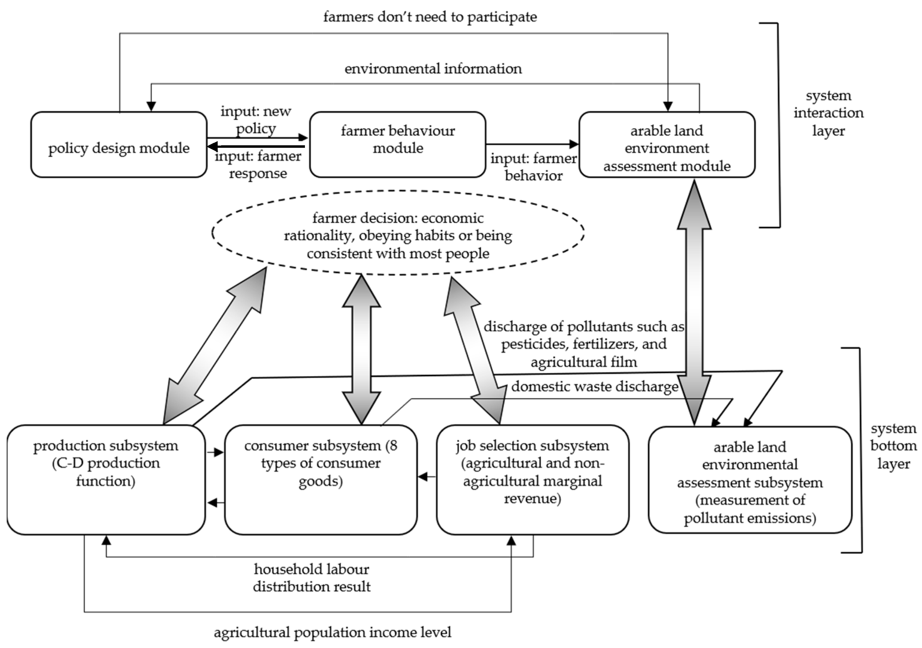
In this paper, Swarm is used as a platform and Java language is used to program the M-ABM model. By simulating the adaptive adjustment process of farmers’ behaviour affected by policy changes, this model can evaluate the impact of policy implementation on farmers and the arable land environment and effectively express the response chain of “policy implementation—farmers’ behavioural change—arable land environment change”. This paper gives a brief description of the basic assumptions, principal rules, system structure, and characteristics of the model.
The M-ABM model employs an “artificial village” of a 60 × 60 grid size (a grid represents one mu of land, totaling 3600 mu of available land, more than half of which is arable) with 200 households, governments, non-agricultural markets, credit institutions, agricultural enterprises, environments, and other subjects living in it. The system can be used to simulate and observe these virtual farmers living in artificial villages. The system includes both the “natural environment” and “social environment”. The farmers grow crops, raise livestock, or go to work and consume. They are affected by policies and environmental factors, and they constantly learn and accumulate from life experiences and the environment. All types of experiences are accumulated, and decision-making and behaviour adapt to achieve the expected higher quality of life. The model includes five preconditions: The boundary condition, diversification assumption of farmers, incomplete rational condition, separability assumption of production, and consumption decision-making and homogeneity assumption of the environment. Farmers’ diversity assumptions are reflected in the family population, age, cultural and educational level, family wealth, income, risk appetite, arable land quality, arable land area, and arable landform characteristics. Incomplete rational conditions mean that every decision of the farmer can be regarded as a choice involving the three directions of economic rationality, obeying habits and obeying most people’s choices. Farmers’ decision-making rules can be summarized as “maximizing income through the rational allocation of resources under various constraints”, and the sum of the behaviours of the farmers’ groups creates the environmental consequences of the model assessment.
The M-ABM model is divided into two parts: The system interaction layer, and the bottom layer of the system, according to the hierarchical structure (see Figure 1). The bottom layer of the system completes the simulation of the behaviour of the farmer and the calculation of the environmental impact. The system interaction layer emphasizes the human-machine using expert knowledge. In the process of integration, this aspect is an important reflection of the feedback of policies on environmental changes in the model. According to the bottom layer of the system, the M-ABM model includes four main subsystems: Farmer production, farmer consumption, employment selection, and arable land environmental assessment. The farmer production subsystem uses the C-D production function to measure the input–output relationship and builds a profit function on this basis. The consumer subsystem uses the extended linear expenditure system model influenced by the additional income class to measure the farmers’ problems and structural changes. The employment selection subsystem comprehensively considers employment probability, outbound cost, management factors, etc. To establish an agricultural–non-agricultural income balance formula to describe the labor distribution of farmers, the environmental assessment subsystem selects typical pollutants of air, water, and solid waste as indicators, and several environmental models are employed, such as a modified model of ammonia emissions from the planting industry based on National Ammonia Reduction Strategy Evaluation System (NARSES), an ammonia emissions inventory from the aquaculture industry based on the material flow method, Intergovernmental Panel on Climate Change (IPCC), Total Nitrogen (TN) estimation formula of the national greenhouse gas inventory guideline catalogue, etc. The simulation starting point of the model is roughly equivalent to 1990, and the monetary values involved are calculated at 1990 prices.
Compared with traditional methods, M-ABM uses multi-agent modeling technology to integrate interdisciplinary methods. By simulating the adaptive response of farmers to policies to assess the environmental impact of policies, it directly connects the whole process from policy implementation to environmental change and solves the problem that the assumptions of pure rationality and homogeneity of farmers commonly used in previous studies do not conform to reality. This approach reduces the dependence on historical information of the rural environment in modelling and analysis and has the ability to perform integrated evaluation that is lacking in the single-subject method.
2.2. Key Formulas and Parameter Descriptions Involved in this Paper
In this paper, the simulation of two policy scenarios of farmland pollution control mainly involves the planting production aspect of the farmer production subsystem and the calculation aspect of farmland environmental pollution in the environmental assessment subsystem. However, the decision-making related to farmer consumption (determining the balance of funds after the farmer meets his or her living expenses in the current period, which will affect the production budget for the next period) and labor distribution (determining the number of laborers invested in crop production in the households during this period) will also have a joint impact on production-related decision-making. Here, the key formulas and parameters of crop production, household consumption, employment choice, and calculation of arable land environmental pollutants are explained.
2.2.1. Production Profit Function of Farmers’ Planting Industries
Based on the total and structural data of main crops in China, this paper designs a virtual crop, which can reflect the relationship between production input and product output of the main crops in China. The basic formula of the profit function of farmers’ planting production is as follows:
where,
Equation (2) is a production function formula, and Equation (1) is a profit function of the planting industry composed of a production function and a cost function; it is the most critical decision-making factor for farmers to make decisions on crop production. Among them, P represents the profit of the farmer’s production, Ps represents the unit price of the sale of the agricultural product, and Ys represents the quantity of the agricultural product. Pfertilizer, Ppesticide, Pagricultural film, Pmachinery, and Pirrigation water respectively represent the purchase price of fertilizer, pesticide, agricultural film, machinery, and irrigation water, which were obtained by actual data processing. xfertilizer, xpesticide, xagricultural film, xmachinery, xirrigation, xarable land, and xlabor represent the inputs of fertilizers, pesticides, agricultural film, machinery, irrigation water, arable land, and labor, respectively. A0 is the agricultural subsidy and net investment value, referring to the current policy and quota of agricultural subsidies in China; the simulation period was shortened to accelerate the accumulation of household wealth. dage is the age of the farmer (the age is divided into five segments: less than or equal to 30 years old, 31–40 years old, 41–50 years old, 51–60 years old, and 60 years old and above; the values of these five segments are included in the model as 2 years, 4 years, 5 years, 4 years, and 3 years, respectively). dedu is the level of cultural education of the farmer households (illiterate, elementary school, junior high school, high school/secondary school, junior college, and above correspond to the cultural education years of 0, 6, 9, 12, and 15 years, respectively). β1–β7 is the output elasticity coefficient corresponding to the seven input factors.
2.2.2. Farmers’ Consumption Function
The design goal of the farmers’ consumption system was to determine how farmers made their own consumption decisions under different income levels, different savings, and the tendency to expand their production inputs. The consumption by farmers of various consumer goods or services will affect the impact of domestic waste on the cultivated environment. Savings and renewable production inputs will have an impact on the changes in the amount of inputs to the arable land in the next phase and will also have an impact on the arable land environment.
At present, there are two types of research on the consumption structure and consumption demand of farmers. One is the extended linear expenditure system, and the other is Linear Approximated/Almost Ideal Demand System (LA/AIDS). Based on the data obtained, this study used a re-expanded linear expenditure system to establish the consumption function of farmers. The specific expression is shown in Equation (3).
Combining the constant term with Equation (3), and then summing up j, the reorganization can describe the basic consumption amount of a consumer’s consumption of the jth consumer goods, as shown in Equation (4).
The farmer’s income is divided into three grades, and the total amount of consumer’s consumption of the jth consumer goods is as shown in Equation (5).
By performing multiple linear regression on Equation (5), we can obtain αj, βj, γj1, and γj2, and we can also obtain the marginal propensity to consume in consideration of income class variables. The basic consumption demand, of the jth type of consumer goods can be calculated and substituted into Formula (4) to obtain the total consumption PjXj of the jth type of consumer goods.
In Equations (3)–(5), αj is a constant and βj is the marginal propensity to consume in excess of the basic consumption needs. The larger the value is, the higher the consumption of farmers and the less funds that can be used for savings and expanded reproduction. Pj is the price of various consumer goods (in this article, according to the “Jiangxi Statistical Yearbook” [22], it mainly includes eight basic consumer goods: food, tobacco, alcohol, clothing, housing, daily necessities and services, transportation and communication, education, culture and entertainment, health care, and other supplies and services). Xj is the consumption of various consumer goods; is the basic consumption demand; is also the basic consumption demand; Y is the income; and Dj is the dummy variable of the income level. In this study, the income level has been divided into three categories: low, medium, and high. When the income is 0 < Y < 1200, the farmer is a low-income household, assuming D1 = 1, D2 = 0; when the income is 1200 ≤ Y ≤ 2500, the farmer is in a middle-income household, assuming D1 = 0, D2 = 0; and when the income is 2500 < Y, the farmer is in a high-income household, assuming D1 = 0, D2 = 1. γjk is the parameter to be evaluated, indicating the correction value of the marginal consumption propensity of j goods or services in addition to the basic consumption expenditures.
This study uses time series data instead of cross-sectional data for calculations, as shown in Appendix A Table A1 (the rightmost two columns in Table A1 are the product of different income groups and their corresponding D1, D2) based on the fact that in recent decades, the changes in farmers’ consumption demand are only related to their income changes and are not influenced by the historical period. Although this assumption is not entirely true, it can basically reflect reality due to the short time span [23,24,25,26,27].
2.2.3. Farmers’ Employment Selection Function
The goal of this part of the design was to determine how farmers choose between agricultural production and non-agricultural production (local odd jobs or field jobs), and it is the marginal benefit of labor that determines the choice of farmers. Generally, the marginal benefit of non-agricultural employment is greater than that of the agricultural sector, which is an important reason for the transfer of a large number of rural workers to cities [28,29,30]. When labor flows to cities, labor in agricultural production is reduced, consumption is reduced, and the pollution of arable land is also reduced. The formulas for determining the labor distribution of farmers in agriculture and non-agricultural employment are as follows:
In Equations (6) and (7), Ragr is the marginal benefit of labor in agricultural production, that is, when the labor in agricultural production is reduced by one, the profit will be reduced; Rnagr is the marginal benefit of the labor force in the non-agricultural employment market; avenagr is the average wage of the non-agricultural employment market; Pnagr is the probability of non-agricultural employment of farmers, affected by age, cultural education level, family-owned arable land area, family wealth, etc.; Ctransport is the transportation cost of non-agricultural employment for farmers; and Cothers is other costs. The greater the gap between Ragr and Rnagr, the more likely it is that farmers will make new employment decisions that are intended to increase income, thus affecting the agricultural production and household income of farmers and further affecting their consumption, and ultimately, the pollution of arable land.
2.2.4. Arable Land Pollution Function
In this part, the main consideration for studying the pollution of arable land was the pollution by agricultural chemicals such as chemical fertilizers and pesticides, with additional considerations of livestock and poultry emissions, crop residues, and living sources in “artificial villages”. Therefore, representative fertilizers, pesticides, livestock and poultry emissions, crop residue sources, and total nitrogen (TN) and total phosphorus (TP) discharged into the water source were indicated. Here, the calculation refers to the N and P emission formulas of the Intergovernmental Panel on Climate Change (IPCC) for domestic sewage. Therefore, the calculation formula for the pollution of nitrogen and phosphorus in arable land in this paper is as follows:
In Equations (8) and (9), N, Ffertilizer, Flivestock, Fcrop residue, and Fsource of life refer to the nitrogen in the leaching and runoff, the amount of nitrogen applied by the virtual fertilizer in the system, the amount of nitrogen emitted by livestock, and the crop, respectively. For the amount of nitrogen in the residue and the amount of nitrogen emitted by farmers, the unit is kilogram N/step, and fN is the rate of nitrogen loss. P, Ffertilizer1, Flivestock1, Fcrop residue1, and Fsource of life1 refer to phosphorus occurring in leaching and runoff during the agricultural process, the amount of phosphorus applied by the virtual fertilizer in the system, the amount of phosphorus emitted by livestock and poultry, the amount of phosphorus in crop residues, and the amount of phosphorus emitted by farmers in their lives, and the unit is kilogram N/step. ffertilizer, flivestock, fcrop residue, and fsource of life are the TP loss rate of chemical fertilizer, the TP loss rate of livestock and poultry, the TP loss rate of crop residues, and the TP loss rate of living sources, respectively. Yang et al. [24] estimated the nitrogen expenditures of the Yangtze River, Yellow River, and Pearl River basin, according to Xing et al. [31], and the overall nitrogen loss rate was 19–23%. Zhu [32] reported that the loss rate of fertilizer nitrogen in arable land is 7%. The research results of the Nanjing Institute of Soil Science of the Chinese Academy of Sciences show that the nitrogen loss rate in the Poyang Lake area is 13.6% to 16.6% [33]. Therefore, the total wastage rate of various types of nitrogen selected in this study was 15%. Ma et al. [34] reported that the loss rate of phosphate fertilizer in arable land is generally less than 5%, and the loss rate of phosphorus runoff is usually much smaller than that of nitrogen. Liu et al. [35] researched the Three Gorges Reservoir Area and showed that the loss of phosphate fertilizer in leaching and runoff is 5.99%. Yang et al. [25] conducted a study on rural non-point source pollution in China. The TP loss rate in this study was 4% for fertilizer and straw sources; livestock and living sources of TP were mainly in the form of organic phosphorus, and their loss rate was relatively high (5%).
2.3. Model Data Description
Two sources of data were used in this section. Chemical fertilizer, pesticide, agricultural film, agricultural diesel, total power of agricultural machinery, irrigation ratio, labor, and per capita net income of rural households were derived from the Jiangxi Statistical Yearbook [22]. The arable land area and multiple cropping index data were derived from the statistical yearbooks of counties and cities in Jiangxi Province, such as the Nanchang Statistical Yearbook [35] and the Ganzhou Statistical Yearbook [36]. The data covers 24 years in Jiangxi Province (1990–2013).
3. Scenario Design of Regulation Policy for Reducing Fertilizer and Pesticide Application on Arable Land
Fertilizer and pesticide sources are the most important sources of nitrogen and phosphorus load on arable land in China [37]. Internationally, the regulation of chemical fertilizers and pesticides mainly adopts economic or market-based measures to guide pollution control by increasing the cost of pollution behaviour or increasing the benefits of environmentally friendly behaviours. The most direct taxation of polluting production involves the method of collecting fertilizer tax, nitrogen tax, phosphorus tax, and adopting subsidies and compensation mechanisms such as ecological compensation [38]. This paper establishes the strategy of arable land pollution control by controlling the application of chemical fertilizers and pesticides. The scenario analysis plan is divided into two sets of scenarios, namely, the collection of fertilizer tax and ecological compensation. The relevant assumptions and sub-scenarios of each scenario are designed as follows.
3.1. Scenario C: Fertilizer Taxation Scenario
This scenario examines the effect of arable land pollution control and the impact on crop production under different tax rates after the levying of a fertilizer tax. The quantitative indicators mainly investigate the application intensity of chemical fertilizer per mu, the loss of arable land pollutants (TN, TP as an indicator), and the scale of planting production (in terms of the number of plots in the planting industry) in artificial villages. We assumed that the cost of the increase in fertilizer tax is borne by the farmers, and a five sub-scenario was designed. They were recorded as the control plan and sub-scenarios C1, C2, C3, and C4. Their corresponding fertilizer tax rates are 0%, 50%, 100%, 150%, and 300%, respectively. Five scenarios of no fertilizer tax, lower tax rate, medium tax rate, higher tax rate, and high tax rate were designed, as shown in Table 1. The purpose was to observe the adaptive response of farmers to policies under different tax rates. That is, when the government implements different levels of fertilizer tax, what agricultural production, consumption, and employment decisions will be made by farmers, and how will these decisions ultimately affect the arable land environment? The current value of the 100-period value is accurate to the actual value of 1990. The control plan and each sub-scenario are executed beginning with simulation phase 101 and run 100 times, that is, run to 200.
In this scenario, the price of virtual crops is still 0.85 yuan/kg. The initial input intensities (1990) of various factors of production in the model were 23.72 kg/mu fertilizer, 1.02 kg/mu pesticide, 0.50 kg/mu plastic film, 0.19 kW/mu agricultural machinery, and 78.2% arable land irrigation. The details are shown in Appendix Table A2.
By calibrating the model 100 to the 2013 situation, we could control the 100-phase. In the benchmark model, 1 yuan is initially used as the stepping scale for farmers to adjust. If the fertilizer, pesticide, and agricultural film application are to be adjusted, the amount corresponding to 1 yuan will increase or decrease each time. While pesticides are the most expensive, the dosage is small. Fertilizers are the cheapest, but the dosage is large. Therefore, the actual situation may vary greatly. Generally, the fertilizer application will be adjusted to be larger than the pesticide application according to the price, and the pesticide application will be larger than the application of agricultural film; for example, if the price of one of these products is low, the tax might be adjusted to 2 yuan, but it might shortly thereafter be adjusted to 0.5 yuan. A certain level will be achieved by repeating the stepping scale of the three elements. Starting from the 101st period, the tax is collected, and the average value of periods 191–200 is calculated.
3.2. Scenario D: Ecological Compensation Scenario
The ecological compensation policy, also referred to herein as the government compensation scenario, refers to the government’s policy of giving certain monetary subsidies to farmers who have a positive effect on the arable land environment.
If farmers reduce the input of fertilizers and pesticides on arable land, it will reduce pollution to arable land and rural environments, which will have positive external effects on the environment but will affect the output of arable land and reduce the income level of farmers. How do we reduce the input of chemical fertilizers and pesticides while ensuring that the income does not decline? This balance requires the government to compensate farmers, and determining the appropriate kind of compensation to achieve the goal of protecting arable land and the environment was the subject of this part of our study.
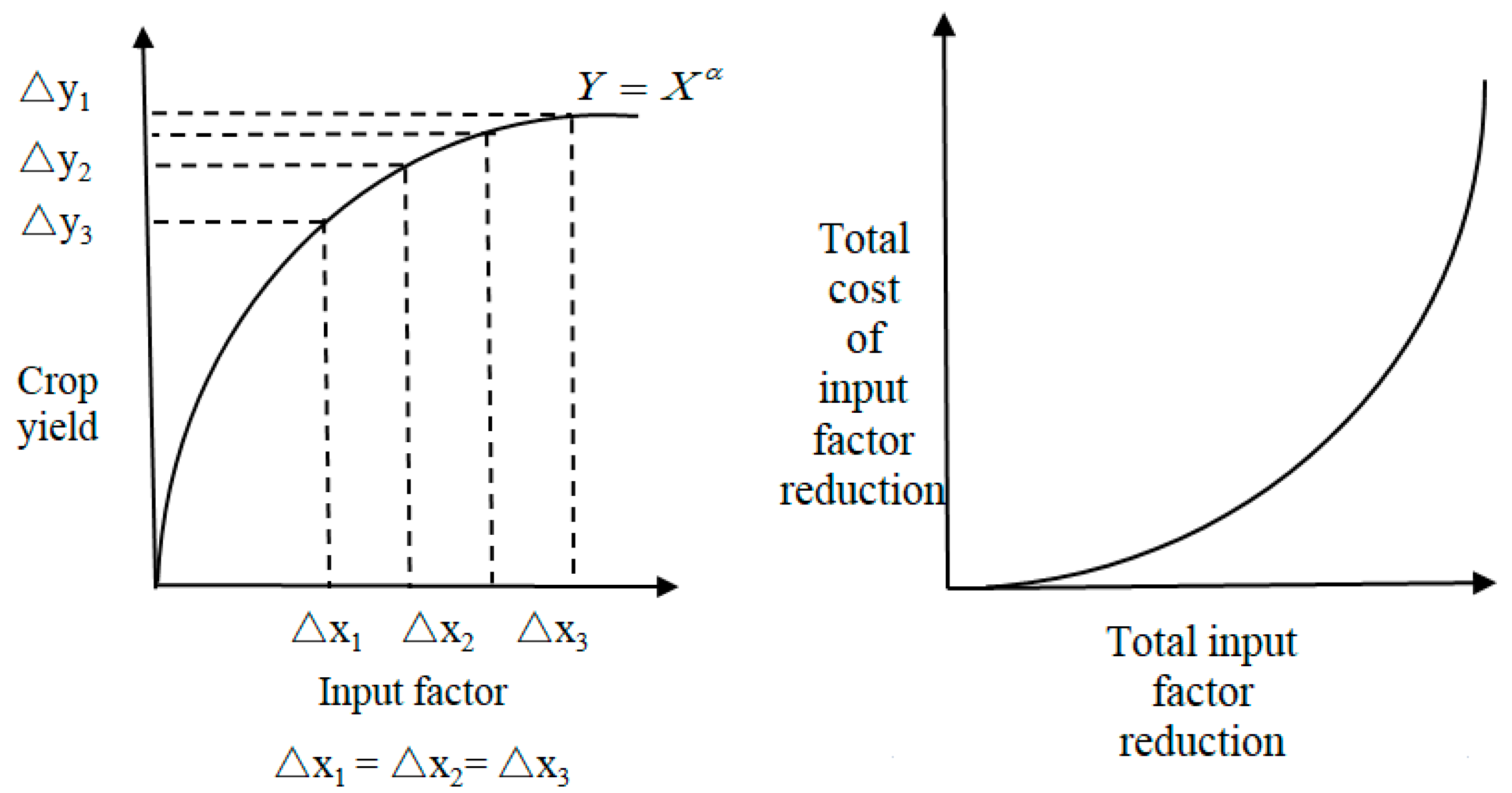
For the input factors of arable land production, if the input of agricultural chemicals such as chemical fertilizers, pesticides, and agricultural film is reduced, the following two results will be produced. On the one hand, the degree of damage to the environment will be reduced, and as the input of these items is reduced, the production costs will also decrease. On the other hand, the reduction in these production-increasing and labor-saving production factors will reduce the output per unit of land and encourage farmers to invest in more labor, which will reduce the income of farmers to a certain extent. The difference between the reduced income of farmers and the input cost of production factors should be compensated by the government to the farmers. The relationship between the cost and the input factors is shown in Figure 2. Because of the reduction in the investment in these agrochemicals, the quality of agricultural products will be improved. In general, high-quality agricultural products will have higher selling unit prices in the market, thus increasing the income of farmers to a certain extent. However, the impact of this aspect complicates the simulation process and is not discussed in this study.
If only the effect of fertilizer and pesticide changes on the output is considered, the farmer’s production function is (where < 1), which is a concave function, as shown in Figure 2. The cost of reducing the input of unit factors is increasing gradually; that is, the decrease in output produced by reducing the input per unit of production factor at a low level is less than the decrease in output caused by reducing the input per unit of production factor at a high level. The marginal cost is rising. The increase in the marginal cost means that from the total reduction of production cost and the total reduction of input factors, as the total amount decreases, the total reduction of production cost also increases, which is a convex function.
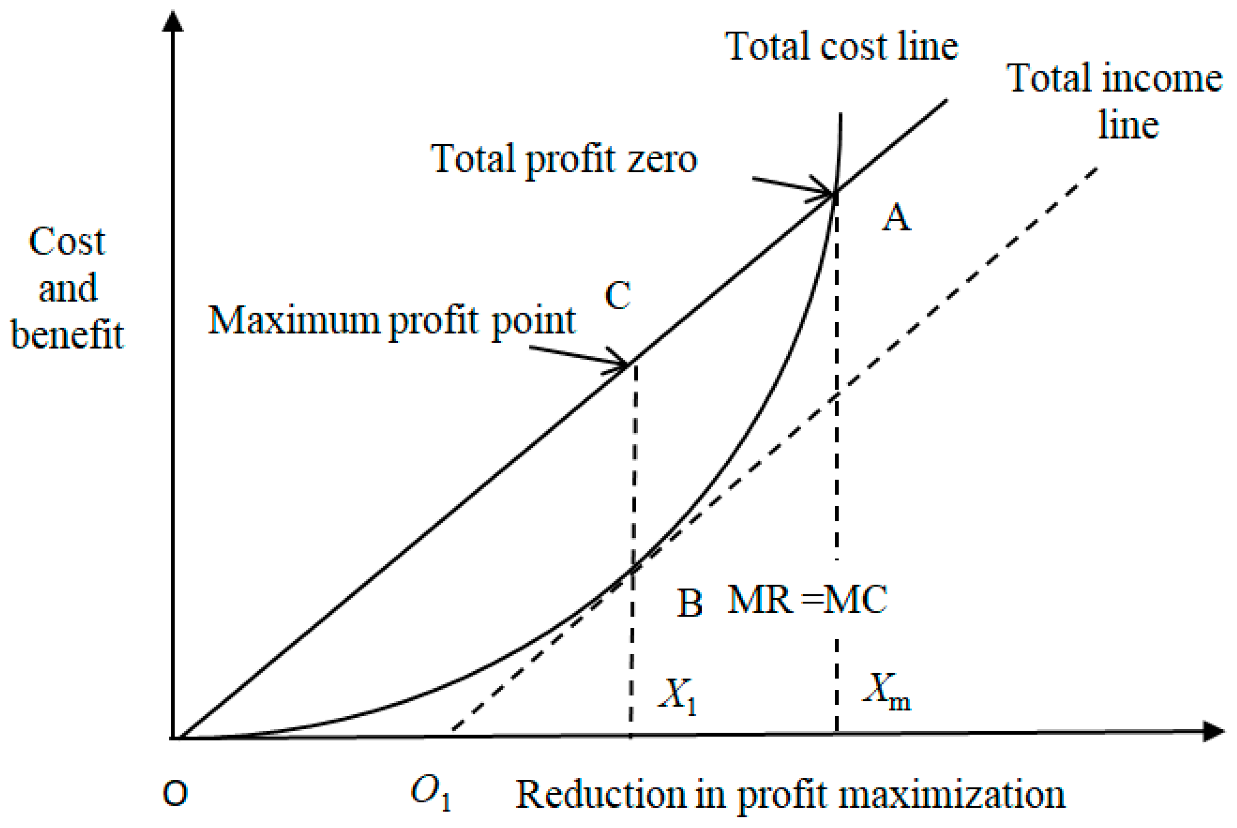
The government will compensate for the loss of, or increase the production cost caused by the reduction of the production factors of the farmer’s household by ecological compensation. This compensation is linear; that is, for every reduction of the input of a unit of production factors, the peasant household will obtain the same subsidy. In this case, the total cost and the total income curves are shown in Figure 3.
In Figure 3, the OA line is the total revenue curve, and the OA arc is the total cost curve. The two lines intersect at point A and are parallel to the vertical axis through point A. The corresponding input factor reduction is , where the parallel line of the OA line is tangent to the total cost curve at point B, parallel to the vertical axis through point B, and intersects with the total income curve at point C; its corresponding input factor reduction is . At point C, farmers will obtain the maximum profit, and point B represents the marginal cost and marginal income being equal; that is, MR = MC. At point A, the total cost is equal to the total income, and farmers obtain the maximum profit at point C.
This paper designs two ecological compensation sub-scenarios: The inertia scenario (anarchic guidance) and government compensation scenario (pure government guidance scenario). Under the pure government guidance scenario, government compensation is divided into two options: Equal compensation (including high compensation and low compensation) and differential compensation. Through scenario analysis, the role of ecological compensation policy in reducing arable land pollution control is illustrated.
Sub-scenario D1: The inertia scenario does not interfere with the production behaviour of farmers and simulates the changing trend of fertilizer and pesticide application levels under the conditions of self-organization and self-adaptation of farmers.
Sub-scenario D2: The government compensation scenario (pure government guidance scenario), in which the government intervenes in fertilizer and pesticide application by farmers through ecological compensation. It is assumed that the sale price of crops is fixed. The farmer’s behaviour of reducing fertilizer and pesticide application is only compensated by the government, and the intensity of fertilizer and application use by farmers is set to X kg/mu and Y kg/mu, respectively. When the amount of fertilizer applied by the farmer and the amount of application are between start-up and moderate, the government will compensate the U1 or V1 for each fertilizer reduction of 1 kg/mu or pesticide reduction of 0.05 kg/mu. When the amount of fertilizer applied by farmers and the amount of application are between moderate and strict, the government will compensate U2 or V2 for each reduction of 1 kg/mu or 0.05 kg/mu, and the compensation for each period will be calculated according to the total amount of reduction. The cost of the reduced application of fertilizer and pesticide by the farmer increases with the amount of application per unit area. Therefore, this scenario considers two cases, namely, equal compensation (U1 = U2, V1 = V2), and differential compensation (U1 < U2, V1 < V2). The equal compensation scenario is implemented to reduce the amount of fertilizers and pesticides used by farmers under the prescribed standards and to purchase the amount of the reduced amount according to the unified standard; that is, the amount of compensation per unit reduction does not change, including high (equal) compensation scenarios and low (equal) compensation scenarios. The former refers to the situation in which under certain environmental management objectives, and in the process of gradual optimization of the scheme, the farmers reduce their use of chemical fertilizers and pesticides under the prescribed standards. The amount of reduction is rewarded at a higher level, while the achievement of a lower standard of reduction is rewarded with a low compensation scenario. The differential compensation scenario refers to the different unit compensation system adopted at different levels due to the difference in the cost (reduced profit) caused by using 1 unit of fertilizer or pesticide per reduction at different levels.
With fertilizer application intensities of 24 kg/mu and 15.33 kg/mu, pesticide application intensities of 1.68 kg/mu and 1.05 kg/mu were used as the control levels and farmers were given subsidies. The changes in fertilizer and pesticide application level and compensation level under the above scenarios were simulated. For the application of chemical fertilizers by farmers at 24–33.403 kg/mu, when the application level is X kg/mu, the farmers are subsidized (33.403 − X) * U1 yuan/mu, which is based on the average level of 33.403 kg/mu. According to the average level of 33.403 kg/mu, for each reduction in the application of 1 kg/mu, U1 is subsidized. For the application of chemical fertilizer by farmers at 15.33–24 kg/mu, when the level of fertilizer application is X kg/mu, the farmers are given a subsidy of (24 − X) * U2 yuan/mu, which is U2 for each reduction of 1 kg/mu according to the average level of 24 kg/mu. For the application of pesticides by farmers at 1.68–2.339 kg/mu, when the level of application is X kg/mu, a subsidy of ((2.339 − X) * V1/0.05) yuan/mu is given; that is, a subsidy of V1 is given for each reduction of 0.05 kg/mu of pesticides applied according to the average level of 2.339 kg/mu. For the application of pesticides by farmers at 1.05–1.68 kg/mu, when the level is X kg/mu, subsidies ((1.68 − X) * V2/0.05) yuan/mu are given. That is, according to the average level of 1.68 kg/mu, every 0.05 kg/mu of pesticides is reduced, and V2 subsidies are given. The model will simulate the two cases of equal subsidy (U1, U2) and differential subsidy (V1, V2).
There are certain common preconditions and assumptions in the two sub-scenarios:
(1) Duration of policy implementation: The starting point of implementing the ecological compensation policy is simulation phase 101. The average application level of fertilizer and pesticide in arable land is 33.4 kg/mu and 2.339 kg/mu, respectively, which is similar to the actual situation in Jiangxi Province in 2013 (the data come from Jiangxi Statistical Yearbook in 2013 [39]). This is defined as the launch level, and each sub-scenario runs to 200.
(2) Simulated expected environmental goals: According to previous studies [40,41], as well as the “Technical Guidelines for Environmental Safety in the Use of Chemical Fertilizers” and “Technical Guidelines for Environmental Safety in the Use of Pesticides” promulgated by China in 2010, the moderate and strict environmental objectives of the models were determined, which corresponded to different levels of fertilizer and pesticide application per unit area. According to the recommended value, the fertilizer application structure of Jiangxi Province (according to the Jiangxi Statistical Yearbook [22], we take the average value from 1990 to 2014) and multiple cropping index (according to the Jiangxi Statistical Yearbook [22], we take the average value from 1990 to 2014) to determine moderate and strict arable land environmental goals, the moderate arable land environment goal is to control the application rate of chemical fertilizers and pesticides to less than or equal to 24 kg/mu and 1.68 kg/mu, respectively; the strict arable land environment goal is to control the application rate of fertilizer and pesticides to less than or equal to 15.33 kg/mu and 1.05 kg/mu, respectively.
3.3. Two Scenarios of Farmers’ Production Decision Formula Transformation
The sub-scenarios C and D mainly interfere with the production process of farmers’ planting industries. This intervention can be expressed as the change of farmers’ profit function and farmers’ marginal income, while the consumption function and labor distribution formula need not be modified and instead respond to the new profit function.
In Scenario C, the profit function of the farmer’s crop production is:
where is the fertilizer tax rate, and is the new price of the virtual crop. It is assumed that in the artificial village, the purchase amount of the virtual crop remains unchanged. The price of the virtual crop was designed according to the supply and demand relationship. When the fertilizer tax policy is implemented, the new price of the virtual crop becomes:
Referring to the current policies and quotas of agricultural subsidies in China, and in order to accelerate the accumulation of household wealth, we shortened the simulation period. In this study, the government compensation for reducing the use of chemical fertilizers and pesticides per mu was set to 10 yuan/mu.
new price of virtual crop = original price of virtual crop × (average of virtual crop yield in artificial village/current crop yield of virtual crop).
In Scenario D, the profit function of farmers’ planting industries was deformed into:
where is the new price of virtual crops, Afertilizer and Apesticide are the government compensation for reducing the use of chemical fertilizers and pesticides per mu, and A0 is set to 10 yuan/mu.
Scenarios C and D both directly influence the farmers’ production decisions through the application of policies, control the intensity of pollution production inputs, and affect the consumption and labor distribution behaviour of farmers, ultimately affecting the reduction of farmland pollution.
4. Simulation Results and Analysis
4.1. Scenario C (Levy Fertilizer Tax) Simulation Results and Analysis
According to the relevant settings of Scenario C, the control plan and sub-scenarios C1, C2, C3, and C4 are trained and simulated for 100 periods each, that is, run to 200 periods, and the simulation results (mean values of periods 191–200) are shown in Table 2.
Compared with the current status of the 100th period, the value of each group of non-levy fertilizer taxes increases significantly. When the fertilizer tax is not levied, the model is allowed to run to the 200th period, and the average of the 191–200 period is calculated. The average fertilizer application intensity per mu, TN loss from fertilizer sources, and TP loss from fertilizer sources were 41.26 kg/mu, 4587.806 kg N/mu, and 293.136 kg P/mu, respectively, which increased by 23.53%, 20.53%, and 20.53% compared with the initial period of taxation. If the input of agricultural chemicals such as fertilizer is not controlled, the average fertilizer application per mu, TN loss from fertilizer sources, and TP loss from fertilizer sources will continue to grow.
The application of chemical fertilizer tax can control arable land pollution to a certain extent compared to the absence of a policy intervention. In sub-scenarios C1 and C2, fertilizer per mu application intensity decreased by 2.91% and 13.04%, TN loss of fertilizer source decreased by 8.49% and 17.60%, and TP loss of fertilizer source decreased by 8.49% and 17.60%, respectively, compared with the initial taxation. Before the 100% tax rate, in sub-scenarios C1 and C2, arable land pollution was sensitive to intensity control, and the planting scale changed randomly. In sub-scenarios C3 and C4, fertilizer per mu application intensity decreased by 10.45% and 7.80%, TN loss of fertilizer source decreased by 19.70% and 29.42%, and TP loss of fertilizer source decreased by 19.70% and 29.42%, respectively, compared with the initial taxation. After the 100% tax rate, in sub-scenarios C3 and C4, arable land pollution was not sensitive to intensity control, and the reduction of planting scale became the main source of TN and TP reduction.
Because the amount of chemical fertilizers, pesticides, and agricultural film has been relatively high at the time of taxation, the taxation is not satisfactory when such high application rates are applied. Even if a 300% tax is levied, the effect is not as good as that of 200% tax, which, in turn, is not as good as a 150% tax, which is not as good as 100% tax. Thus, a higher tax rate does not induce a better effect. When the tax rate is too high, the smaller scale of planting will threaten food security. This is mainly because the fertilizer tax is levied when the fertilizer application rate is high, which will greatly increase the agricultural production cost of the farmers. In particular, with the cost of fertilizer, the burden on farmers will increase greatly, and some farmers with lower marginal output will give up farming and switch employment. Although the control effect of a higher tax rate on the input of chemical fertilizers and pesticides per mu of arable land will be weakened, the control effect on the pollution of arable land in the whole village will be strengthened. The main reason is that some of the farmers withdraw from farming so that the planting area of the whole village is reduced, or the input of production factors such as fertilizer is reduced, ultimately bringing the pollution of arable land under control.
In summary, when the fertilizer tax policy is implemented, as the tax rate increases, the effect may not be better. When the average amount of fertilizer at the initial taxation point is already high, the medium tax rate will be more effective than the high tax-rate option. After exceeding the 100% tax rate, further improvements are not achieved. The reduction in the planting scale becomes the main source of TN and TP reduction. That is, the implementation of a high-tax policy can effectively control TN and TP in arable land pollution, but mainly from reducing the planting scale.
4.2. Scenario D (Ecological Compensation) Results and Analysis
According to scenario D, in contrast to sub-scenario D0 (inertial scenario), sub-scenario D1 simulates the implementation of the government ecological compensation policy from phase 101. According to different environmental objectives, the simulation results are summarized into the following four schemes. The simulation results are shown in Table 3.
Option 0: Sub-scenario D0, which is the inertial scenario without any government action;
Option 1: Sub-scenario D1, which is a government equivalent compensation scenario, and the model reaches the moderate standard when it runs to phase 200;
Option 2: Sub-scenario D1, which is a government equivalent compensation scenario, and the model reaches a strict standard when it runs to phase 200;
Option 3: Sub-scenario D1, which is the government differential compensation scenario, and meets strict standards when the model runs to phase 200.
As shown in Table 3, the government intervention scenarios are obviously more effective than the inertial scenario without any government intervention; that is, sub-scenario D1 is better than sub-scenario D0. When the model was run to the 200th period, the application intensity of arable land fertilizer per mu, the application intensity of pesticide per mu, the loss of TN of the chemical fertilizer source, and the loss of TP were higher than those in option 1, and the high values were 74.10% (17.56 kg/mu), 59.27% (0.99 kg/mu), 114.84% (2452.35 kg), and 18.46% (45.68 kg/mu), respectively.
For the same amount of compensation, the high compensation scenario (option 2) is superior to the low compensation scenario (option 1). When the model is run to the 200th period, option 1 is higher than option 2 in terms of the application intensity of fertilizer, the application intensity of the pesticide, the loss of the fertilizer source TN, and the loss of the chemical fertilizer source TP, and the high values are 55.63% (8.47 kg/mu), 58.87% (0.62 kg/mu), 60.62% (802.96 kg), and 60.26% (93.05 kg), respectively. However, the compensation/income ratio of option 2 is 24.3%, which is 16.2% higher than the 8.1% of option 1.
The differential compensation scenario (option 3) is better than the equal compensation scenario (option 1 and option 2). Because option 2 is superior to option 1, only option 3 and option 2 need to be compared here. When the model is run to the 200th period, the application intensity of the fertilizer and the application intensity of the pesticides in option 3 are lower than that of option 2, and the low values are 0.51% (0.08 kg/mu) and 1.95% (0.02 kg/mu), respectively. The planting area of the 200th period of option 3 (1496 mu) is larger than the planting area of option 2 (1408 mu); although the intensity per unit area of option 3 is slightly lower, the total loss of TN and TP is relatively higher, and the high compensation scenario reduces the planting scale of the artificial villages. Therefore, although the intensity of the unit area under the government scenario is slightly lower, the loss of TN and TP is relatively higher because of the larger planting scale. That is, comparing low government compensation with high government compensation and comparing low government compensation with differential government compensation, the reason why high government compensation has a better control effect on TN and TP is that it reduces the planting scale in artificial villages. In terms of government compensation and income ratio, that of option 3 is 21.4%, which is lower than that of option 2 (24.3%). Option 3 is more effective than option 2 for lightening the government burden.
In summary, the government compensation scenario is superior to the inertia scenario; under the premise of government compensation, the high equal compensation scenario is better than the low equal compensation scenario, and the differential compensation scenario is superior to the high equal compensation scenario. The differential compensation can lighten the government burden.
5. Conclusions and Policy Recommendations
This paper adopted multi-agent modelling technology based on the complex adaptive system theory, and took farmers as the research unit, analyzed the impact of policy implementation on arable land environments by simulating the behaviour of farmers, and established “artificial villages” of 200 households and other simulated agents. In this “artificial village”, farmers had arable land, housing, etc. Through adaptive learning and reactions, the artificial village quantitatively expressed the whole process of farmer production, consumption, and employment and their impact on the arable land environment. This model could effectively reflect changes in farmers’ decision-making and assess the environmental impact on arable land. The model design in this paper followed the model boundary constraints, the diversity of farmers, the incomplete rationality of farmers’ behaviour, the separability of production and consumption, and the assumption of environmental homogeneity. The behaviour of farmers followed the resource allocation rules, production decision rules, consumption decision rules, and employment selection decision rules. Based on the above, this paper simulated a total of nine sub-scenarios of fertilizer tax and ecological compensation policies. The five sub-scenarios under the fertilizer tax policy—the inertia scenario, low tax rate (50% tax rate), medium tax rate (100% tax rate), medium and high tax rate (150% tax rate), and high tax rate (300% tax rate)—and the four sub-scenarios under the ecological compensation policy—the inertial scenarios, government equal compensation scenarios to achieve moderate targets, government equal compensation scenarios to achieve strict targets, and government differential compensation scenarios to achieve strict targets—were included. Under the implementation of the simulation policy, farmers will be able to re-evaluate their production, consumption, and employment selection decisions through the re-allocation of resources to maximize utility and ultimately have a different impact on arable land and the rural environment. The model achieves two management objectives: One is a moderate management goal, and the other is a strict management goal. Based on the above analysis, this paper has the following conclusions:
(1) In agricultural production, farmers allocate resources through repeated adaptation and learning to achieve the proximity of all factor configurations and ideal optimal values. However, the adjustment of the allocation of such resources has led to the use of a large number of modern agricultural production factors, while the rural areas in Jiangxi Province lack the supporting management methods which have had huge negative impact on the arable land environment, causing a serious threat to the environmental security of arable land.
(2) Fertilizer tax policies and ecological compensation policies have alleviated the pollution of fertilizer and pesticide input factors to arable land environments to a certain extent.
(3) When the government implements the chemical fertilizer tax policy, as the tax rate increases, the effect may not be better. When the average amount of fertilizer per mu at the initial tax point is already high, the medium tax rate will be more effective than the high tax rate option. Although the high-tax scheme produces greater reductions in TN and TP than do the low and medium tax rates, the amount of fertilizer and pesticide used per mu is higher in the high-tax scheme than with the low and medium tax rates. The implementation of the high-tax scheme pushes some farmers with lower marginal revenues out of the arable land cultivation industry and into aquaculture or non-agricultural industries. In this case, the reduction of the planting scale becomes the main source of TN and TP reduction. That is, the implementation of a high-tax policy can effectively control TN and TP in arable land pollution but mainly from the shrinkage of the planting scale. This effect will threaten food security in Jiangxi Province, so the medium tax rate is more appropriate.
(4) At the time of implementation of the ecological compensation policy, the amount of arable land per unit area subjected to the application of fertilizers and pesticides by farmers will further increase under the inertia scenario. Through the implementation of ecological compensation policies, farmers’ production behaviour can achieve higher levels of environmental goals. The government compensation scenario is superior to the inertia scenario; the high government compensation scenario is superior to the low government compensation scenario; the differential government compensation scenario is superior to the equal government compensation scenario; and the differential compensation policy can lighten the government burden. Therefore, the government can implement the protection of the arable land environment by implementing a differential compensation option.
Based on the above conclusions, the following policy implications can be drawn:
(1) For increasingly affluent rural areas, although the rural population has been greatly reduced as the labor force has been transferred to cities and towns, arable land has become increasingly threatened by changes in modern life and production methods. It is recommended that the relevant departments establish corresponding modern rural waste disposal methods, publicize the negative impacts of modern agricultural production factors on the arable land environment, and raise environmental awareness among the rural population. Ultimately, our rural environment and arable land environment will be effectively protected.
(2) The results of the scenario analysis show that the reduction in fertilizers and pesticides will reduce the yield per unit area of crops and, at the same time, reduce the scale of crop production, have a greater impact on food production, and further affect food security. It is recommended that relevant departments coordinate environmental safety and food safety objectives and vigorously carry out agricultural technical training. The first need is to establish a broadcasting station for agricultural technology promotion and timely dissemination of agricultural technology in different periods of crop growth. For example, in the growing period of crops with severe pests in previous years, the dissemination of relevant knowledge before the arrival of the same period of the year, the promotion of technical knowledge, and effective prevention of pests and diseases will reduce the input intensity of agrochemicals, protecting the arable land environment while increasing production. The second need is to propose the development of new agricultural technologies and increase the input of new harmless or low-harm production factors to increase production. The third is to implement regional rotation-based production restriction policies and control arable land pollution through regional food production and consumption accounting.
Author Contributions
H.X. and G.L. had the original idea for the study; G.L. was responsible for data collecting, and carried out the analyses; H.X. and G.L. drafted the manuscript.
Funding
This study was supported by the National Natural Science Foundation of China (No. 71864017) and the Research Projects of Humanities and Social Sciences in Colleges and Universities of Jiangxi Province (No. JJ162004).
Acknowledgments
This paper expresses our heartfelt thanks to Yang Shunshun, a researcher of Hunan Academy of Social Sciences, who has provided strong support and help for the software application of this model.
Conflicts of Interest
The authors declare no conflict of interest.
Appendix A

Table A1.
Consumption data of 24 groups of households to be regressed (converted to 1990 levels, unit: yuan).
Table A1.
Consumption data of 24 groups of households to be regressed (converted to 1990 levels, unit: yuan).
| Serial Number | Per Capita Net Income | Total Living Consumption | Pixi | D1Y | D2Y | |||||||
|---|---|---|---|---|---|---|---|---|---|---|---|---|
| Food, Tobacco, Alcohol | Clothes | Life | Daily Necessities and Services | Traffic Communication | Education, Culture and Entertainment | Healthcare | Other Supplies and Services | |||||
| 1 | 669.90 | 576.69 | 368.68 | 35.37 | 48.14 | 53.50 | 7.50 | 42.50 | 17.50 | 3.50 | 669.90 | 0.00 |
| 2 | 693.51 | 589.34 | 372.49 | 38.21 | 44.29 | 53.33 | 11.35 | 44.92 | 18.78 | 5.97 | 693.51 | 0.00 |
| 3 | 732.90 | 618.29 | 383.41 | 38.85 | 93.80 | 27.30 | 9.95 | 42.20 | 18.00 | 4.79 | 732.90 | 0.00 |
| 4 | 737.43 | 603.68 | 370.34 | 35.83 | 80.64 | 30.20 | 14.57 | 43.89 | 20.83 | 7.38 | 737.43 | 0.00 |
| 5 | 815.15 | 689.97 | 433.04 | 39.25 | 87.18 | 32.57 | 15.45 | 51.37 | 19.65 | 11.45 | 815.15 | 0.00 |
| 6 | 879.25 | 718.37 | 443.01 | 40.19 | 95.85 | 33.10 | 18.47 | 53.46 | 22.58 | 11.70 | 879.25 | 0.00 |
| 7 | 984.60 | 817.91 | 497.93 | 45.92 | 113.55 | 38.09 | 22.16 | 63.47 | 25.14 | 11.66 | 984.60 | 0.00 |
| 8 | 1086.93 | 809.37 | 475.48 | 39.89 | 117.91 | 36.79 | 21.04 | 72.37 | 30.54 | 15.35 | 1086.93 | 0.00 |
| 9 | 1045.90 | 785.57 | 459.30 | 34.26 | 113.11 | 34.21 | 20.63 | 82.16 | 28.17 | 13.74 | 1045.90 | 0.00 |
| 10 | 1108.55 | 836.80 | 480.07 | 35.64 | 119.59 | 35.94 | 28.72 | 89.38 | 31.83 | 15.63 | 1108.55 | 0.00 |
| 11 | 1121.69 | 862.91 | 469.89 | 44.35 | 117.64 | 29.13 | 50.22 | 96.78 | 33.35 | 21.55 | 1121.69 | 0.00 |
| 12 | 1181.74 | 910.81 | 469.16 | 48.38 | 138.98 | 31.13 | 60.06 | 103.81 | 38.35 | 20.95 | 1181.74 | 0.00 |
| 13 | 1237.30 | 945.97 | 474.04 | 51.62 | 139.51 | 32.85 | 66.79 | 114.43 | 42.93 | 23.81 | 0.00 | 0.00 |
| 14 | 1294.91 | 1005.13 | 519.57 | 52.61 | 139.17 | 33.03 | 74.66 | 117.92 | 48.47 | 19.70 | 0.00 | 0.00 |
| 15 | 1503.14 | 1082.72 | 588.71 | 54.57 | 119.48 | 34.05 | 87.51 | 120.80 | 56.16 | 21.43 | 0.00 | 0.00 |
| 16 | 1626.68 | 1237.23 | 607.99 | 62.03 | 162.49 | 48.00 | 114.37 | 137.62 | 77.05 | 27.68 | 0.00 | 0.00 |
| 17 | 1757.56 | 1318.32 | 649.35 | 64.27 | 183.11 | 51.81 | 123.03 | 140.96 | 78.03 | 27.76 | 0.00 | 0.00 |
| 18 | 1898.99 | 1387.69 | 691.43 | 68.45 | 219.89 | 56.33 | 128.44 | 117.14 | 77.72 | 28.31 | 0.00 | 0.00 |
| 19 | 2047.74 | 1442.65 | 711.96 | 68.77 | 243.87 | 67.57 | 131.52 | 102.89 | 89.67 | 26.41 | 0.00 | 0.00 |
| 20 | 2230.29 | 1552.48 | 707.19 | 71.45 | 318.66 | 79.95 | 129.98 | 111.96 | 102.30 | 31.00 | 0.00 | 0.00 |
| 21 | 2462.61 | 1664.11 | 771.15 | 74.28 | 332.99 | 87.33 | 141.16 | 121.34 | 103.74 | 32.11 | 0.00 | 0.00 |
| 22 | 2776.40 | 1877.39 | 848.61 | 94.10 | 358.09 | 111.80 | 158.46 | 128.67 | 139.67 | 37.99 | 0.00 | 2776.40 |
| 23 | 3061.71 | 2006.43 | 873.42 | 103.63 | 402.96 | 108.86 | 193.41 | 134.04 | 148.81 | 41.30 | 0.00 | 3061.71 |
| 24 | 3337.92 | 2582.45 | 961.94 | 129.05 | 644.60 | 140.91 | 257.21 | 224.64 | 177.16 | 46.95 | 0.00 | 3337.92 |
Table A2.
Means of current input factors.
| Year | Fertilizer (suffix, kg) | Pesticide (kg) | Agricultural Film (kg) | Machinery Power (kg) | Effective Irrigation Ratio (%) |
|---|---|---|---|---|---|
| 1990 | 836,000,000 | 35,879,000 | 17,505,000 | 6,677,167 | 78.2 |
| 1991 | 932,000,000 | 35,879,000 | 17,505,000 | 6,692,285 | 78.8 |
| 1992 | 941,000,000 | 34,485,000 | 16,907,000 | 6,345,786 | 79.4 |
| 1993 | 938,000,000 | 34,250,000 | 16,932,000 | 6,306,139 | 80.1 |
| 1994 | 1,048,000,000 | 37,998,000 | 20,500,000 | 6,438,156 | 80.8 |
| 1995 | 1,121,000,000 | 41,932,000 | 21,785,000 | 6,630,750 | 81.4 |
| 1996 | 1,127,000,000 | 44,482,000 | 21,105,000 | 6,913,258 | 82.1 |
| 1997 | 1,204,000,000 | 45,259,000 | 24,792,000 | 7,500,270 | 82.7 |
| 1998 | 1,131,000,000 | 48,704,000 | 27,509,000 | 7,939,078 | 83.2 |
| 1999 | 1,167,000,000 | 54,502,000 | 30,256,000 | 8,530,196 | 83.7 |
| 2000 | 1,069,000,000 | 51,406,000 | 28,599,000 | 9,023,070 | 84.5 |
| 2001 | 1,097,000,000 | 51,384,000 | 30,778,000 | 10,020,350 | 83.4 |
| 2002 | 1,124,000,000 | 57,323,000 | 35,407,000 | 11,118,200 | 88.5 |
| 2003 | 1,110,000,000 | 53,470,000 | 33,930,000 | 12,205,200 | 88.9 |
| 2004 | 1,235,000,000 | 66,273,000 | 42,828,000 | 14,652,000 | 88.8 |
| 2005 | 1,294,000,000 | 75,305,000 | 45,010,000 | 17,812,600 | 87.3 |
| 2006 | 1,326,000,000 | 75,955,000 | 40,854,000 | 21,370,850 | 86.3 |
| 2007 | 1,326,508,000 | 88,833,000 | 38,071,000 | 25,063,200 | 85.7 |
| 2008 | 1,330,000,000 | 96,662,000 | 41,645,000 | 29,464,300 | 65.1 |
| 2009 | 1,358,000,000 | 97,593,000 | 43,719,000 | 33,589,300 | 65.3 |
| 2010 | 1,376,000,000 | 107,000,000 | 45,491,000 | 38,050,000 | 65.7 |
| 2011 | 1,411,000,000 | 99,691,000 | 47,375,000 | 42,000,000 | 66.2 |
| 2012 | 1,413,000,000 | 100,000,000 | 50,275,000 | 45,996,850 | 67.6 |
| 2013 | 1,416,000,000 | 99,922,000 | 51,401,000 | 20,141,320 | 70.8 |
References
- Kuang, F. Difference analysis of farmers’ knowledge and protection behaviour of ecological environment—Taking the use of pesticide and chemical fertilizer as an example. Res. Soil Water Conserv. 2018, 25, 321–326. [Google Scholar]
- Bao, X. Fertilizer, environment and sustainable development of Chinese agriculture. Stat. Decis. 2007, 1, 73–74. [Google Scholar] [CrossRef]
- Wang, Y.; Peng, Z. Effects of excessive fertilization on soil ecological environment of protected arable land. J. Agro-Environ. Sci. 2005, 24, 81–84. [Google Scholar]
- Li, L. Study on the Impact of Utilization of Production Factors on Grain Yield and Environment—Taking Fertilizer as an Example; China Agricultural University: Beijing, China, 2015. [Google Scholar]
- Zhu, H.; Sun, M. Review of land use intensification research and future work focus. Acta Geogr. Sin. 2014, 69, 1346–1357. [Google Scholar]
- Scott, D.; Cooper, P.; Lake, S.; Sabater, S.; Melack, J.M.; Sabo, J.L. The effects of land use changes on streams and rivers in Mediterranean climates. Hydrobiologia 2013, 719, 383–425. [Google Scholar]
- Guo, J.H.; Liu, X.J.; Zhang, Y.; Shen, J.L.; Han, W.X.; Zhang, W.F.; Christie, P.; Goulding, K.W.; Vitousek, P.M.; Zhang, F.S. Significant acidification in major Chinese croplands. Science 2010, 327, 1008–1010. [Google Scholar] [CrossRef] [PubMed]
- Zhu, Z.; Sun, B.; Yang, L.; Zhang, L.X. Control policies and measures for agricultural non-point source pollution in China. Sci. Technol. Rev. 2005, 23, 47–51. [Google Scholar]
- Zhang, W.L.; Xu, A.G.; Ji, H.J.; Kolbe, H. Estimation and control countermeasures of agricultural non-point source pollution in China III—Analysis of existing problems in agricultural non-point source pollution control in China. Chin. Agric. Sci. 2004, 37, 1026–1033. [Google Scholar]
- Xie, X.; Chen, M.; Li, Z. Comparative study on arable land quality protection behaviour of different groups of farmers—Based on the perspective of pesticides and fertilizers. Rural. Econ. Technol. 2016, 27, 12–16. [Google Scholar]
- Wang, Z. China’s Agricultural Environmental Policy Research Based on the Perspective of Agricultural Support; Graduate School of the Chinese Academy of Agricultural Sciences: Beijing, China, 2013. [Google Scholar]
- Li, K.; Ma, D. Study on the fertilizer input and decision-making mechanism of farmers in ecologically fragile areas—Taking 421 households in 4 counties of Shanxi Province as an example. J. Nanjing Agric. Univ. (Soc. Sci. Ed.) 2018, 18, 138–160. [Google Scholar] [CrossRef]
- Geng, F.; Luo, L. Study on farmers’ willingness to reduce chemical fertilizer consumption and use organic fertilizer—From the perspective of non-point source pollution prevention and control in the upper reaches of Erhai river basin. Chin. J. Agric. Resour. Reg. Plan. 2018, 39, 74–82. [Google Scholar]
- Guo, Q.H.; Li, S.P.; Li, H. Adoption behaviours of farmers’ chemical fertilizer reduction measures based on the perspective of social norms. J. Arid Land Resour. Environ. 2018, 32, 50–55. [Google Scholar] [CrossRef]
- Wang, T. Research on Influencing Factors of Implementing Three Reductions by Rice Growers in Sanjiang Bureau of Agricultural Reclamation and Construction; Heilongjiang Bayi Agricultural Reclamation University: Daqing, China, 2017. [Google Scholar]
- Zeng, W. Study on Ecological Compensation for Fertilizer Reduction Based on Farmers’ Willingness; Kunming University of Technology: Kunming, China, 2014. [Google Scholar]
- Ge, J. Economic Research on Agricultural Non-Point Source Pollution and Treatment in Jiangsu Province; Nanjing Agricultural University: Nanjing, China, 2011. [Google Scholar]
- Zhang, L. Effect of vertical cooperative mode on the behaviour of chemical fertilizer application of rice farmers: Based on the survey data of 189 farmers in Jiangxi Province. Agric. Econ. Probl. 2008, 3, 50–54. [Google Scholar] [CrossRef]
- Jin, S.; Zhou, F. Zero growth of chemical fertilizer and pesticide use: China’s objectives, progress and challenges. J. Resour. Ecol. 2018, 9, 50–58. [Google Scholar]
- Lou, B. Research on Farmers’ Production Behaviour Based on Agricultural Product Quality and Safety; Chinese Academy of Agricultural Sciences: Beijing, China, 2015. [Google Scholar]
- Li, H. Building an Economic Incentive Mechanism and Service System to Solve the Problem of Agricultural Non-point Source Pollution; Fudan University: Shanghai, China, 2011. [Google Scholar]
- Statistical Bureau of Jiangxi. Jiangxi Statistical Yearbook; China Statistics Press: Beijing, China, 1991–2014.
- Herbert, A.S. Practice-based Microeconomics; Gezhi Publishing House: Shanghai, China, 2009. [Google Scholar]
- Cheng, Z. Simulation Analysis of Food Policy Effects Based on Farmers’ Subjects; Graduate School of the Chinese Academy of Social Sciences: Beijing, China, 2010. [Google Scholar]
- Yang, S.; Yan, S. Rural Environmental Management Simulation—Simulation Analysis of Farmers’ Behaviour; Science Press: Beijing, China, 2012. [Google Scholar]
- Zhang, Q. Econometric analysis of the consumption structure of agricultural village residents in China. Anhui Agric. Sci. Bull. 2007, 13, 20–21. [Google Scholar]
- Ma, L. ELES analysis of rural residents’ consumption structure in Ningxia. Inn. Mong. Sci. Technol. Econ. 2007, 23, 2–3. [Google Scholar]
- Lewis, G.J. Human Migration; Groom Helm Ltd.: London, UK, 1982. [Google Scholar]
- Lee Everett, S. A Theory of Migration. Demography 1966, 3, 47–57. [Google Scholar]
- Xin, M. Labor Market Reform in China; Cambridge University Press: Cambridge, UK, 2000. [Google Scholar]
- Xing, G.X.; Zhu, Z.L. Regional nitrogen budgets for China and its major watersheds. Bigeochemistry 2002, 57, 405–427. [Google Scholar] [CrossRef]
- Zhu, Z. Rational use of chemical fertilizers and full use of organic fertilizers to develop environmentally friendly fertilization systems. Chin. Acad. Sci. (Proc. Chin. Acad. Sci.) 2003, 2, 89–93. [Google Scholar]
- Whipple, W.; Hunter, J. Nonpoint sources and planning for water pollution control. Water Pollut. Control Fed. 1977, 49, 152. [Google Scholar]
- Ma, B.; Liu, Y.; Xue, J. Analysis of fertilizer application and nitrogen and phosphorus loss in rice-wheat rotation area in southern Hebei. J. Irrig. Drain. 2007, 26, 72–74. [Google Scholar]
- Statistical Bureau of Nanchang. Nanchang Statistical Yearbook; China Statistics Press: Beijing, China, 1991–2014.
- Statistical Bureau of Ganzhou. Ganzhou Statistical Yearbook; China Statistics Press: Beijing, China, 1991–2014.
- Liu, G.; Zhao, Z.; Li, Q. The current situation of agricultural non-point source pollution in the Three Gorges Reservoir Area and its prevention and control measures. Chin. J. Eco-Agric. 2004, 12, 172–175. [Google Scholar]
- Milder, J.C.; Scherr, S.J.; Bracer, C. Trends and future potential of payment for ecosystem services to alleviate rural poverty in developing countries. Ecol. Soc. 2010, 15, 4. [Google Scholar] [CrossRef]
- Statistical Bureau of Jiangxi. Jiangxi Statistical Yearbook; China Statistics Press: Beijing, China, 2014.
- Yang, S.; Luan, S. Simulation of non-point source pollution control in cropping based on multi-agent model: Comparison of the effect of environmental service payment by chemical fertilizer tax. Syst. Eng. Theory Pract. 2014, 34, 777–786. [Google Scholar]
- Zhu, Z.; Jin, J. Fertilizer use and food security in China. Plant Nutr. Fertil. Sci. 2013, 19, 259–273. [Google Scholar]
Figure 1.
Conceptual framework of the simulation model.

Figure 2.
Loss map generated by reducing the production methods of agrochemical input factors.

Figure 3.
Point map of compensation, cost, and profit extremes for farmers to cut production factor inputs.
Figure 3.
Point map of compensation, cost, and profit extremes for farmers to cut production factor inputs.

Table 1.
Scenario design for fertilizer tax policy collection.
| Option Number | Initial | Tax Rate |
|---|---|---|
| Current 100th period value | ||
| Control plan | No fertilizer tax policy | 0% |
| Sub-scenario C1 | Tax collection starts from the 101st period | 50% |
| Sub-scenario C2 | Tax collection starts from the 101st period | 100% |
| Sub-scenario C3 | Tax collection starts from the 101st period | 150% |
| Sub-scenario C4 | Tax collection starts from the 101st period | 300% |
Table 2.
Comparison of fertilizer tax policy and simulation results of each sub-scenario.
| Tax Rate | Fertilizer Application Intensity (kg/mu) | Pesticide Application Intensity (kg/mu) | Agricultural Film Application Intensity (kg/mu) | Fertilizer Source TN Loss (kg N/mu) | Fertilizer Source TP Loss (kg P/mu) | Number of Planting Plots (mu) | |
|---|---|---|---|---|---|---|---|
| Current 100th Period value | - | 33.403 | 2.339 | 1.208 | 3806.281 | 243.201 | - |
| Control plan | 0% | 41.264 | 2.652 | 1.616 | 4587.806 | 293.136 | 1458 |
| Sub-scenario C1 | 50% | 32.430 | 2.517 | 1.541 | 3483.124 | 222.553 | 1408 |
| Sub-scenario C2 | 100% | 29.048 | 2.473 | 1.521 | 3136.408 | 200.400 | 1416 |
| Sub-scenario C3 | 150% | 29.912 | 2.478 | 1.527 | 3056.377 | 195.286 | 1340 |
| Sub-scenario C4 | 300% | 30.797 | 2.493 | 1.509 | 2686.530 | 171.655 | 1144 |
Table 3.
Simulation results of the ecological compensation policy.
| Option Number | Sub-Scenario Number | “Artificial Village” Fertilizer Application Intensity (Kg/Mu) | “Artificial Village” Pesticide Application Intensity (Kg/Mu) | Compensation Situation (Except for One Item in the Form Below, the Unit is Yuan.) | TN Loss of Fertilizer Sources in “Artificial Villages” (Kg) | TP Loss of Fertilizer Sources in Artificial Villages (Kg) | Number of Planting Plots/Mu | |||||
|---|---|---|---|---|---|---|---|---|---|---|---|---|
| U1 | U2 | V1 | V2 | Compensation per mu | Compensation/Income Ratio (%) | |||||||
| Current 100th Period value | - | 33.4 | 2.34 | - | - | - | - | - | - | 3806.28 | 243.2 | - |
| Option 0 | Sub-scenario D0 | 41.26 | 2.65 | 0 | 0 | 0 | 0 | 0 | 0 | 4587.81 | 293.14 | - |
| Option 1 | Sub-scenario D1 | 23.7 | 1.67 | 2.35 | 2.35 | 0.65 | 0.65 | 36.18 | 8.1 | 2135.46 | 247.46 | 1450 |
| Option 2 | Sub-scenario D1 | 15.23 | 1.05 | 4.05 | 4.05 | 1.5 | 1.5 | 112.06 | 24.3 | 1332.46 | 154.41 | 1408 |
| Option 3 | Sub-scenario D1 | 15.15 | 1.03 | 2.8 | 4.2 | 0.75 | 1.7 | 95.17 | 21.4 | 1408.48 | 163.21 | 1496 |
© 2018 by the authors. Licensee MDPI, Basel, Switzerland. This article is an open access article distributed under the terms and conditions of the Creative Commons Attribution (CC BY) license (http://creativecommons.org/licenses/by/4.0/).
Share and Cite
MDPI and ACS Style
Liu, G.; Xie, H. Simulation of Regulation Policies for Fertilizer and Pesticide Reduction in Arable Land Based on Farmers’ Behavior—Using Jiangxi Province as an Example. Sustainability 2019, 11, 136. https://doi.org/10.3390/su11010136
AMA Style
Liu G, Xie H. Simulation of Regulation Policies for Fertilizer and Pesticide Reduction in Arable Land Based on Farmers’ Behavior—Using Jiangxi Province as an Example. Sustainability. 2019; 11(1):136. https://doi.org/10.3390/su11010136
Chicago/Turabian StyleLiu, Guiying, and Hualin Xie. 2019. "Simulation of Regulation Policies for Fertilizer and Pesticide Reduction in Arable Land Based on Farmers’ Behavior—Using Jiangxi Province as an Example" Sustainability 11, no. 1: 136. https://doi.org/10.3390/su11010136
Note that from the first issue of 2016, this journal uses article numbers instead of page numbers. See further details here.