Analysing the Synergies and Trade-Offs between Ecosystem Services to Reorient Land Use Planning in Metropolitan Bilbao (Northern Spain)

 ,
,
Abstract
:1. Introduction
- (1)
- Map these eight ES to explore their spatial distribution.
- (2)
- Identify the most relevant areas for the provision of multiple ES and areas that are mostly lacking ES provision, identifying the corresponding land use type.
- (3)
- Identify existing ES trade-offs and synergies so that managers can prioritize preservation efforts of land use types in the rest of the study area.
- (4)
- Offer recommendations to reorient land use planning practices to maximize ES delivery in the BMG.
2. Methodology
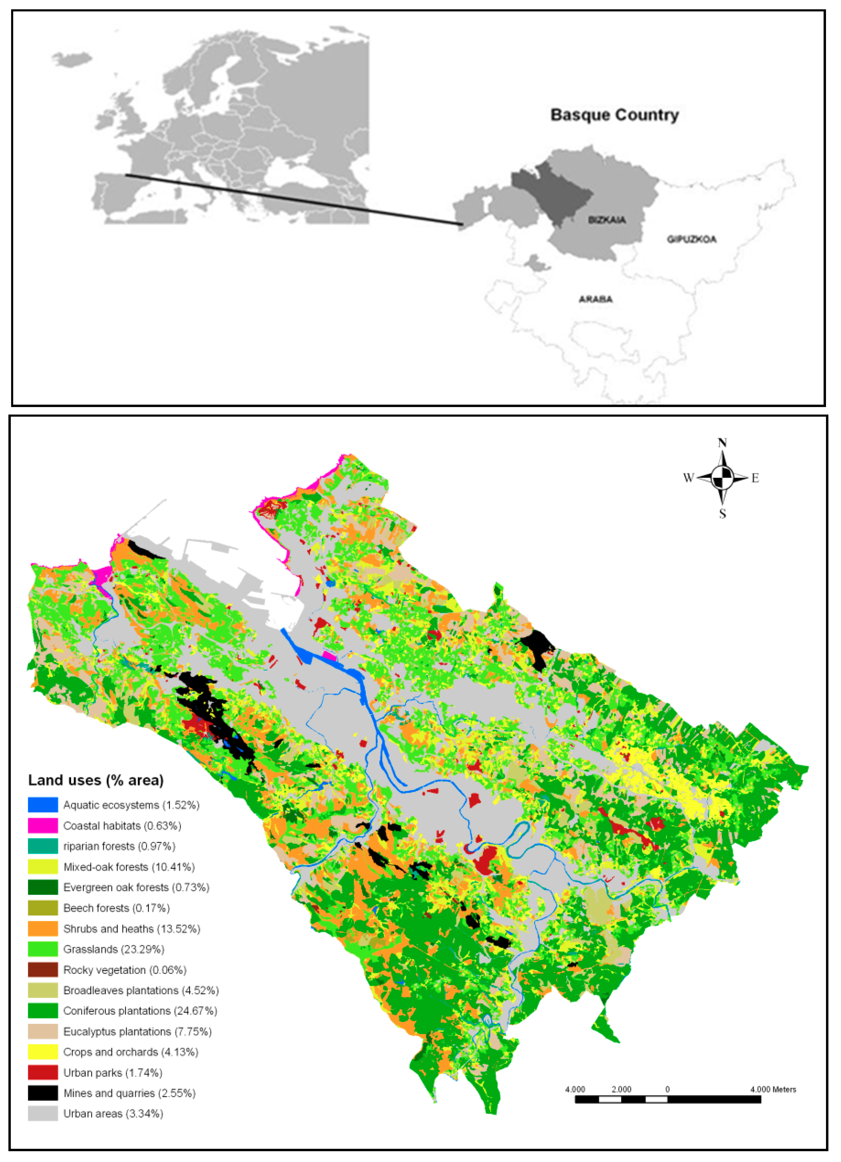
2.1. Study Area
2.2. Selection of Ecosystem Services and Land Use Units
2.3. Mapping and Evaluating Selected ES
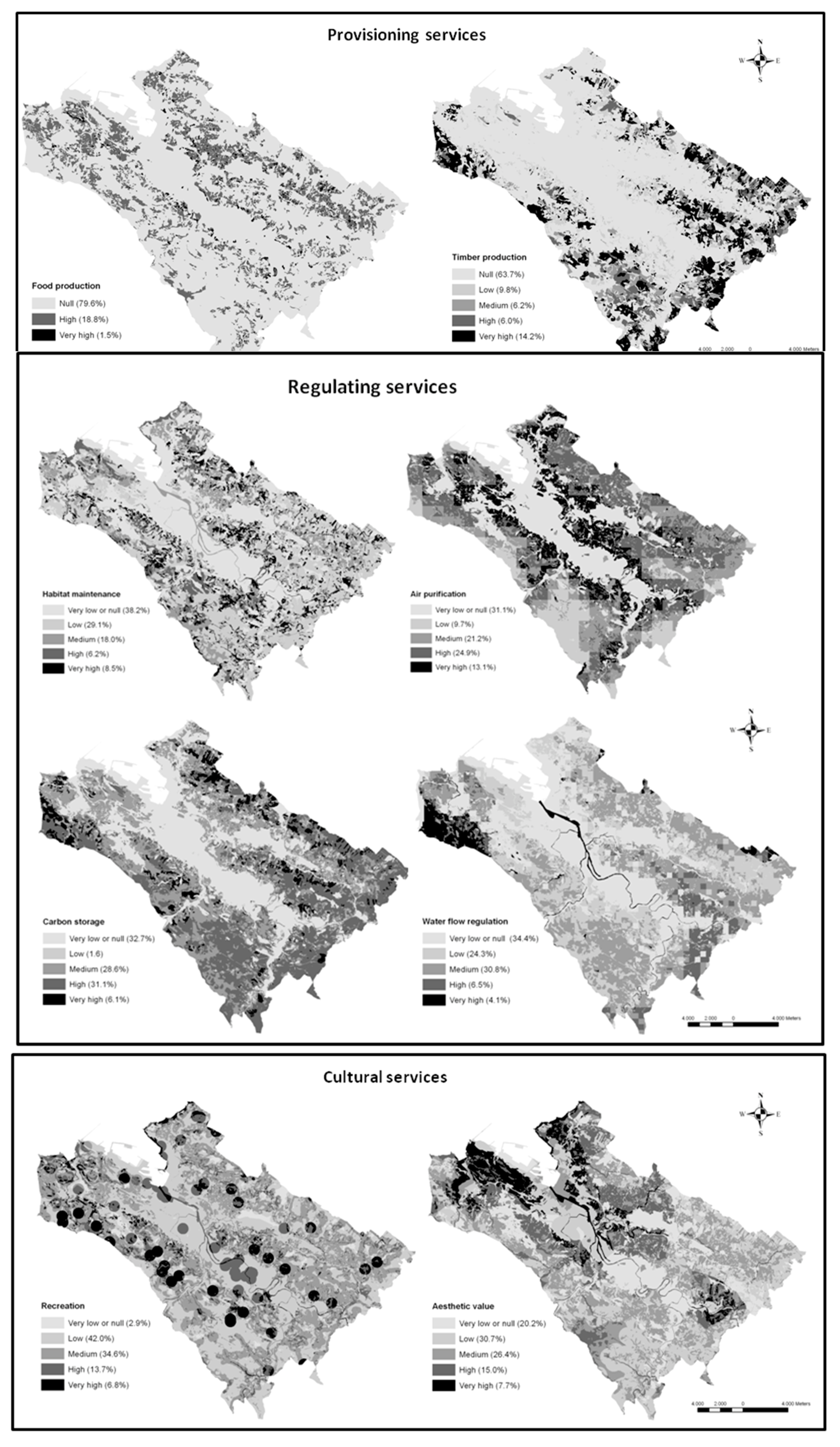
2.3.1. Provisioning ES
Food Production
Timber Production
2.3.2. Regulation ES
Habitat Maintenance
Air Purification
Carbon Storage
Water Flow Regulation
2.3.3. Cultural ES
Recreation
Aesthetic Value
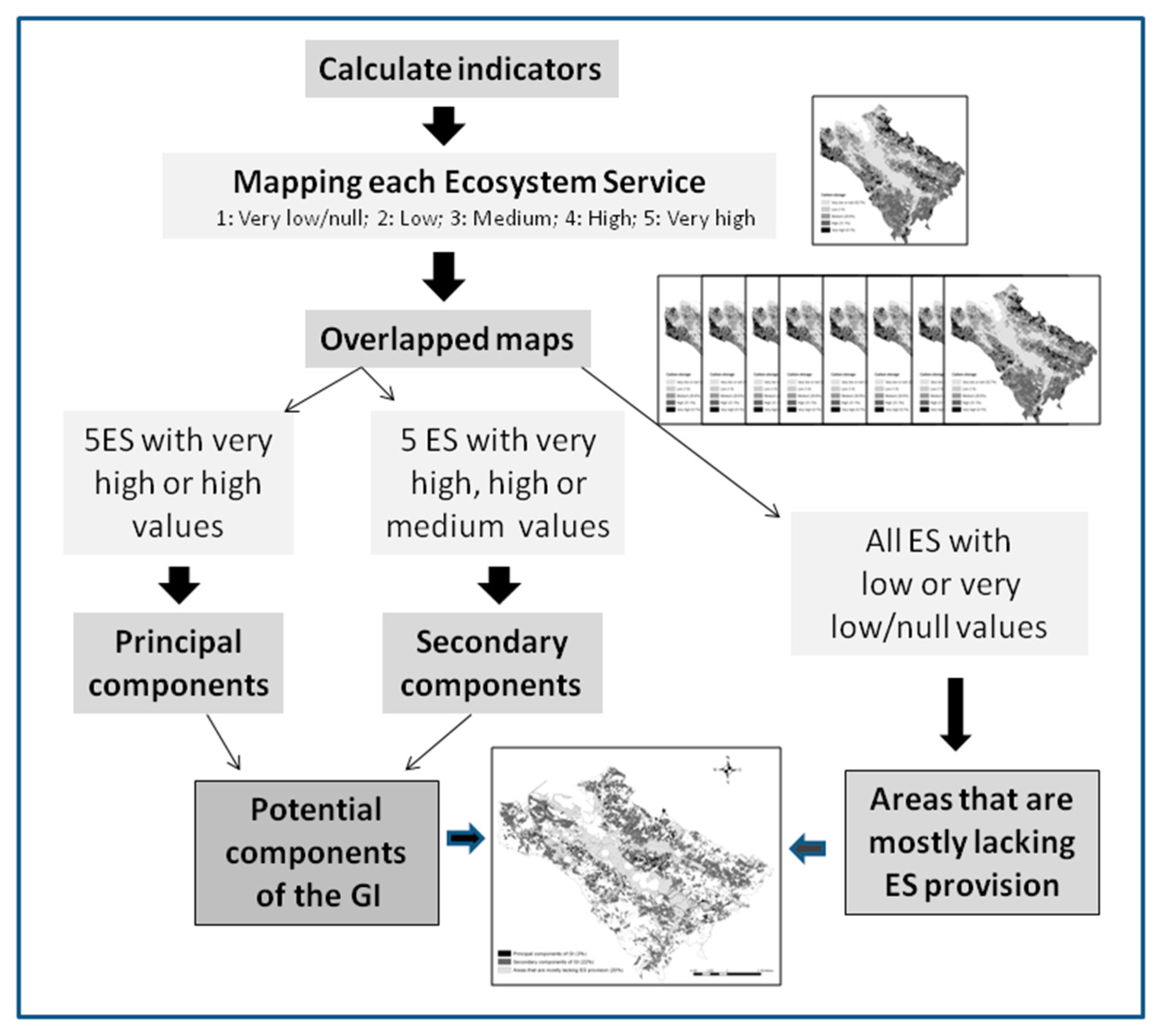
2.4. Data Analysis
3. Results
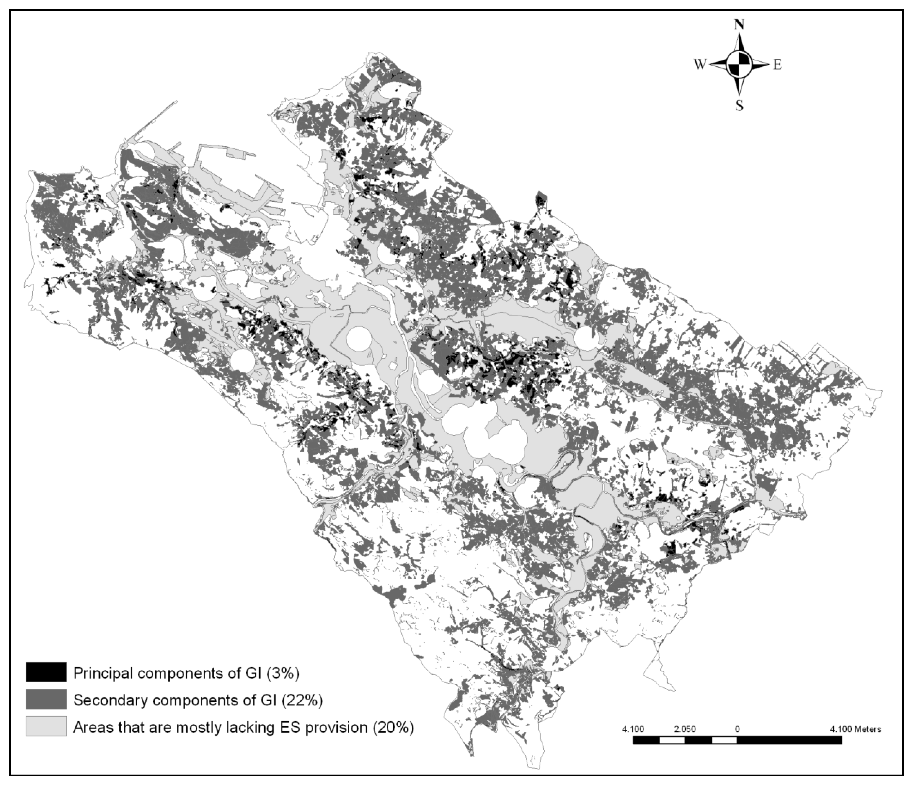
3.1. Mapping and Evaluating Selected ES
3.2. Analysis of Synergies and Trade-Offs
4. Discussion
4.1. Provision of Multiple ES
4.2. Trade-Offs, Synergies and Bundles of ES
4.3. Application of the ES Approach to the Management of Metropolitan Areas. Planning for the Delivery of Multiple ES
5. Conclusions
Author Contributions
Funding
Acknowledgments
Conflicts of Interest
Appendix A

| Ecosystem Service | Indicators | Variables Used to Calculate Indicators | Equations | |
|---|---|---|---|---|
| Provisioning | Food production | Food productivity (F) (tonnes ha−1) | Ap = Agricultural productivity (tonnes ha−1) | F = Ap + Lp Ap = Pa/Sa Lp = M/St |
| Pa = Agricultural production (tonnes) | ||||
| Sa = Surface of agricultural areas (ha) | ||||
| Lp = Livestock productivity (tonnes ha−1) | ||||
| M = Meat production (tonnes) | ||||
| St = Surface of pasture (ha) | ||||
| Timber production | Annual growth of the different forest plantations (m3 ha−1year−1) | |||
| Regulating | Habitat maintenance | Habitat maintenance index (H) | Rp = Native plant species richness | H = Rp + Q + Ni |
| Q = Habitat quality | ||||
| Ni = Sites of natural interest | ||||
| Air purification | Annual NO2 removal (Ra)(g m−2 h−1) | T = NO2 concentration (g m−3) | Ra = T·Vd | |
| Vd = NO2 dry deposition velocity on vegetation (m s−1) | ||||
| Carbon storage | Carbon storage (C) (tC ha−1) | B = Carbon stocks in living biomass (tonnesC ha−1) | C = B + S B = V·α·(1 + β)·Dw·Y | |
| V = Merchantable volume (m3 ha−1) | ||||
| α = Biomass expansion factor | ||||
| β = Root-to-shoot ratio | ||||
| Dw = Basic wood density (tonnes dry matter m−3 merchantable volume) | ||||
| Y = Carbon fraction of dry matter (tonnesC/tonnes dry matter) | ||||
| S = Carbon stored in soil (tonnesC ha−1) | ||||
| Water flow regulation | Water flow regulation index (W) (mm year−1) | U = Water storage in the soil (mm year−1) | W = U/(K − E) | |
| K = Annual rainfall (mm year−1) | ||||
| E = Corrected annual potential evapotranspiration (mm year−1) | ||||
| Cultural | Recreation | Recreation index (F) | Z = Recreation potential | F = Z + O Z = J + X + Wb + G + Ms O = Pr + I |
| J = Degree of naturalness | ||||
| X = Presence of protected areas | ||||
| Wb = Presence of water bodies | ||||
| G = Presence of Sites of Geological Interest | ||||
| Ms = Presence of mountain summits | ||||
| O = Recreation opportunity | ||||
| Pr = Presence of roads and paths | ||||
| I = Presence of infrastructure used for recreation activities | ||||
| Aesthetic value | Aesthetic index (A) | P = Perceived value of landscape units by the Basque population | A = P + R + D + Wb + L + N | |
| R = Relief | ||||
| D = Diversity of landscapes | ||||
| Wb = Presence of water bodies | ||||
| L = Influence of landmarks | ||||
| N = Influence of negative elements in the landscapes | ||||
| Types of Crop | Agricultural Productivity (A) (tonnes ha−1) | Types of Livestock | Meat Production (M) (tonnes) | Area (ha) | Livestock Productivity (L) (tonnes ha−1) |
|---|---|---|---|---|---|
| Orchards | 1576 | Bovine | 5.337 | - | - |
| Fruit trees | 762 | Ovine | 82 | - | - |
| Kiwi crops | 1075 | Equine | 29 | - | - |
| Vineyards | 590 | TOTAL | 5.449 | - | - |
| Land use type | Grasslands | - | 42.616 | 0.13 | |
| Land Uses Types | Air Purification | Carbon Storage |
|---|---|---|
| NO2 Dry Deposition Velocity (m s−1) | Living Biomass (tonnesC ha−1) | |
| Aquatic ecosystems | 0.00 | - |
| Coastal habitats | 0.00 | - |
| Riparian forests | 0.13 | 74 |
| Mixed-oak forests | 0.13 | 115 |
| Evergreen oak forests | 0.28 | 100 |
| Beech forests | 0.13 | 160 |
| Shrubs and heaths | 0.06 | - |
| Grasslands | 0.11 | - |
| Rocky vegetation | 0.00 | - |
| Broadleaves plantations | 0.13 | 106 |
| Coniferous plantations | 0.09 | 81 |
| Eucalyptus plantations | 0.13 | 222 |
| Crops and orchards | 0.10 | - |
| Urban parks | 0.03 | - |
| Mines and quarries | 0.00 | - |
| Urban areas | 0.00 | - |
| Data | Data Source | Description | Indicator Levels | |
|---|---|---|---|---|
| Recreation potential | Degree of naturalness | Values have been adjusted from [84] | Index of degree of human influence on ecosystems. It comprises the damage or transformations caused by humans and how these ecosystems depend on human activity themselves [84] | 7: Natural forests, Rocky vegetation; 6: Coastal habitats; 5: Aquatic ecosystems, Shrubs and heaths; 4: Grasslands; 3: Forest plantations; 2: Urban parks; 1: Crops and orchards, Mines and quarries; 0: Urban areas |
| Presence of protected areas or Sites of Naturalistic Interest | Basque Government (ftp.geo.euskadi.net/cartografia/) | Presence of protected areas or sites of naturalistic interest | 1: Natura 2000 network and Sites of naturalistic interest; 0: No protected areas or without naturalistic interest. | |
| Presence of Water bodies | Basque Government (ftp.geo.euskadi.net/cartografia/) | Presence of rivers, water bodies, coastline related to recreation (bathing water, fishing, and beaches) | 3: Beaches; 2: Water bodies used for fishing or bathing; 1: Water bodies no used for fishing or bathing; 0: no Water bodies | |
| Presence of Sites of Geological Interest | Basque Government (ftp.geo.euskadi.net/cartografia/) | Presence of sites of geological interest with recreational value. | 1: Sites of geological interest with recreational value ≥2; 0: Sites of geological interest with recreational value <2 | |
| Presence of mountain summit | Basque Government (ftp.geo.euskadi.net/cartografia/) (www.mendikat.net) | Presence of mountain summit and a buffer of 500 m. | 1: Buffer of 500 m around the mountain summit; 0: no mountain summits | |
| Recreation opportunity | Accessibility of the site | Basque Government (ftp.geo.euskadi.net/cartografia/) | Presence of roads and paths. | 2: Buffer of 200 m around accessible roads to motor vehicles (highways, roads, etc.); 1: Buffer of 200 m around limited roads to motor vehicles (paths, trails, bike paths); 0: no presence of roads and paths. |
| Infrastructures | Basque Government (ftp.geo.euskadi.net/cartografia/) | Presence of infrastructure used for recreation activities | 3: Buffer of 500 m around constructed infrastructures (recreational areas, wine cellars, museums, ecological parks, theme parks and centers, interpretation centers, bird observatories, landmarks and biking centers), natural infrastructures (caves and climbing sites). |
| Data | Data Source | Description | Indicators Levels |
|---|---|---|---|
| Social perception | Our elaboration based on the EUNIS and social preferences based on mail-in photo-questionnaires | Social preferences of different land uses types for their aesthetic value | 5: Natural forests, Rocky vegetation, Coastal habitats, Aquatic ecosystems, heaths, Grasslands; 4: Shrubs, Coniferous plantations, Crops and orchards, Urban parks; 3: Eucalyptus plantations, Urban areas; 2: Mines and quarries |
| Relief | Basque Government (ftp.geo.euskadi.net/cartografia/) | Index of relief for each viewshed [93] | 1: Viewshed with index of relief ≥32; 0: Viewshed with index of relief <32. |
| Diversity of landscapes | Basque Government (ftp.geo.euskadi.net/cartografia/) | Index of landscape diversity (ILD) for each viewshed [93] | 1: Viewshed with ILD ≥1.70; 0: Viewshed with ILD <1.70. |
| Presence of Water bodies | Basque Government (ftp.geo.euskadi.net/cartografia/) | Presence of rivers, water bodies, coastline, reservoirs. | 1: Landscapes with coastline influence; buffer of 50 m around the river; buffer of once the radius of water bodies and reservoirs; 0: No water bodies or buffers outside our own viewshed. |
| Visual influence of landmarks | Basque Government (ftp.geo.euskadi.net/cartografia/) | 1: Buffer of 2000 m around the landmark; 0: No visual influence of landmark. | |
| Visual influence of negative elements | Basque Government (ftp.geo.euskadi.net/cartografia/) | 1: Buffer of 4000 m around wind farms; buffer of once the diameter of actives quarries around them; buffer of once the radius of landfills; buffer of 2000 m around highways and double carriageways; buffer of 750 m around other roads; buffer of 200 m around railroads and funicular; 0: no visual influence of negative elements. |
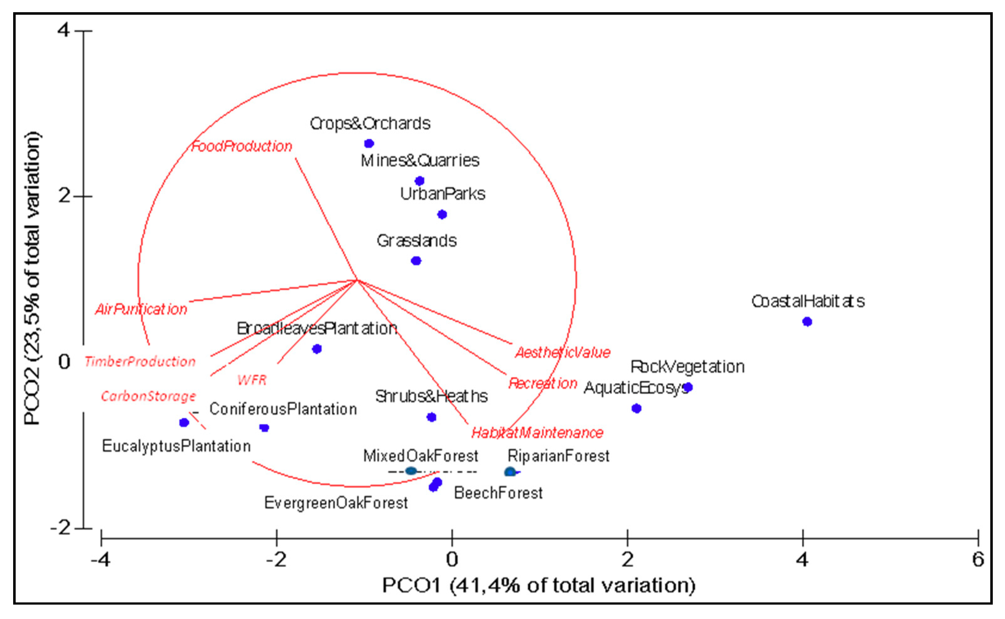
| Factor Scores | |||
|---|---|---|---|
| F1 | F2 | F3 | |
| Ecosystem Services | |||
| Food production | −0.28 | 0.59 | −0.70 |
| Timber production | −0.79 | −0.44 | 0.15 |
| Air purification | −0.77 | −0.11 | −0.55 |
| Carbon storage | −0.77 | −0.53 | −0.20 |
| WFR | −0.44 | −0.49 | 0.22 |
| Habitat maintenance | 0.51 | −0.70 | −0.25 |
| Recreation | 0.68 | −0.46 | −0.30 |
| Aesthetic value | 0.71 | −0.31 | −0.33 |
| Eigenvalue | 46.41 | 2.085 | 1.152 |
| Variance explained (%) | 41.44 | 29.783 | 16.453 |
| Variance accumulated (%) | 41.44 | 67.985 | 84.437 |
References
- Chan, K.M.A.; Shaw, M.R.; Cameron, D.R.; Underwood, E.C.; Daily, G.C. Conservation planning for ecosystem services. PLoS Biol. 2006, 4, e379. [Google Scholar] [CrossRef] [PubMed]
- Rodríguez, J.P.; Beard, T.D.; Bennett, E.M.; Cumming, G.S.; Cork, S.J.; Agard, J.; Dobson, A.P.; Peterson, G.D. Trade-offs across space, time, and ecosystem services. Ecol. Soc. 2006, 11, 28. [Google Scholar] [CrossRef]
- Bennett, E.M.; Peterson, G.D.; Gordon, L.J. Understanding relationships among multiple ecosystem services. Ecol. Lett. 2009, 12, 1394–1404. [Google Scholar] [CrossRef] [PubMed] [Green Version]
- Polasky, S.; Nelson, E.; Pennington, D.; Johnson, K.A. The Impact of Land-Use Change on Ecosystem Services, Biodiversity and Returns to Landowners. A Case Study in the State of Minnesota. Environ. Resour. Econ. 2011, 48, 219–242. [Google Scholar] [CrossRef]
- Turkelboom, F.; Thoonen, M.; Jacobs, S.; Berry, P.; García-Llorente, M.; Martín-López, B. Ecosystem service trade-offs and synergies Ecosystem service trade-offs and synergies. Ecol. Soc. 2015. [Google Scholar] [CrossRef]
- Baral, H.; Keenan, R.J.; Fox, J.C.; Stork, N.E.; Kasel, S. Spatial assessment of ecosystem goods and services in complex production landscapes: A case study from southeastern Australia. Ecol. Complex. 2013, 13, 35–45. [Google Scholar] [CrossRef]
- Hails, R.S.; Ormerod, S.J. Ecological science for ecosystem services and the stewardship of Natural Capital. J. Appl. Ecol. 2013, 50, 807–811. [Google Scholar] [CrossRef] [Green Version]
- Cheung, W.W.L.; Sumaila, U.R. Trade-offs between conservation and socio-economic objectives in managing a tropical marine ecosystem. Ecol. Econ. 2008, 66, 193–210. [Google Scholar] [CrossRef]
- Turkelboom, F.; Leone, M.; Jacobs, S.; Keleme, E.; García-Llorente, M.; Baró, F.; Termansen, M.; Barton, D.N.; Berry, P.; Stange, E.; et al. When we cannot have it all: Ecosystem services trade-offs in the context of spatial planning. Ecosyst. Serv. 2018, 29, 566–578. [Google Scholar] [CrossRef]
- Martínez-Harms, M.J.; Balvanera, P. Methods for mapping ecosystem service supply: A review. Int. J. Biodivers. Sci. Ecosyst. Serv. Manag. 2012, 8, 17–25. [Google Scholar] [CrossRef]
- Burkhard, B.; Kroll, F.; Nedkov, S.; Müller, F. Mapping ecosystem service supply, demand, and budgets. Ecol. Indic. 2012, 21, 17–29. [Google Scholar] [CrossRef]
- Maes, J.; Egoh, B.; Willemen, L.; Liquete, C.; Vihervaara, P.; Schägner, J.P.; Grizzetti, B.; Drakou, E.G.; La Notte, A.; Zulian, G.; et al. Mapping ecosystem services for policy support and decision making in the European Union. Ecosyst. Serv. 2012, 1, 31–39. [Google Scholar] [CrossRef] [Green Version]
- Kroll, F.; Müller, F.; Haase, D.; Fohrer, N. Rural-urban gradient analysis of ecosystem services supply and demand dynamics. Land Use Policy 2012, 29, 521–535. [Google Scholar] [CrossRef]
- Sherrouse, B.C.; Clement, J.M.; Semmens, D.J. A GIS application for assessing, mapping, and quantifying the social values of ecosystem services. Appl. Geogr. 2011, 31, 748–760. [Google Scholar] [CrossRef]
- Koschke, L.; Fürst, C.; Frank, S.; Makeschin, F. A multi-criteria approach for an integrated land-cover-based assessment of ecosystem services provision to support landscape planning. Ecol. Indic. 2012, 21, 54–66. [Google Scholar] [CrossRef]
- Metzger, M.J.; Rounsevell, M.D.A.; Acosta-Michlik, L.; Leemans, R.; Schrotere, D. The vulnerability of ecosystem services to land use change. Agric. Ecosyst. Environ. 2006, 114, 69–85. [Google Scholar] [CrossRef]
- Bryan, B.A. Incentives, land use, and ecosystem services: Synthesizing complex linkages. Environ. Sci. Policy 2013, 27, 124–134. [Google Scholar] [CrossRef]
- De Groot, R.S.; Alkemade, R.; Braat, L.; Hein, L.; Willemen, L. Challenges in integrating the concept of ecosystem services and values in landscape planning, management and decision making. Ecol. Complex. 2010, 7, 260–272. [Google Scholar] [CrossRef]
- Carpenter, S.R.; DeFries, R.; Dietz, T.; Mooney, H.A.; Polasky, S.; Reid, W.V.; Scholes, R.J. Millennium Ecosystem Assessment: Research needs. Science 2006, 314, 257–258. [Google Scholar] [CrossRef] [PubMed]
- Chisholm, R.A. Trade-offs between ecosystem services: Water and carbon in a biodiversity hotspot. Ecol. Econ. 2010, 68, 1973–1987. [Google Scholar] [CrossRef]
- García-Nieto, A.P.; García-Llorente, M.; Iniesta-Arandia, I.; Martín-López, B. Mapping forest ecosystem services: From providing units to beneficiaries. Ecosyst. Serv. 2013, 4, 126–138. [Google Scholar] [CrossRef]
- Geneletti, D. Assessing the impact of alternative land-use zoning policies on future ecosystem services. Environ. Impact Assess. Rev. 2013, 40, 25–35. [Google Scholar] [CrossRef]
- Onaindia, M.; Fernández de Manuel, B.; Madariaga, I.; Rodríguez-Loinaz, G. Cobenefits and trade-offs between biodiversity, carbon storage and water flow regulation. For. Ecol. Manag. 2013, 289, 1–9. [Google Scholar] [CrossRef]
- Balzan, M.; Caruana, J.; Zammit, A. Assessing the capacity and flow of ecosystem services in multifunctional landscapes: Evidence of a rural-urban gradient in a Mediterranean small island state. Land Use Policy 2018, 75, 711–725. [Google Scholar] [CrossRef]
- Baró, F.; Palomo, I.; Zulian, G.; Vizcaino, P.; Haase, D.; Gómez-Baggethum, E. Mapping ecosystem service capacity, flow and demand for landscape and urban planning: A case study in the Barcelona metropolitan region. Land Use Policy 2016, 57, 405–417. [Google Scholar] [CrossRef]
- Baró, F.; Gómez-Baggethun, E.; Haase, D. Ecosystem service bundles along the urban-rural gradient: Insights for landscape planning and management. Ecosyst. Serv. 2017, 24, 147–159. [Google Scholar] [CrossRef]
- Beichler, B.A.; Bastian, O.; Haase, D.; Heiland, S.; Kabisch, N.; Müller, F. Does the Ecosystem Service Concept Reach Its Limits in Urban Environments? Landsc. Online 2017, 51, 1–21. [Google Scholar] [CrossRef]
- Mele, R.; Poli, G. The effectiveness of geographical data in multicriteria evaluation of landscape services. Data 2017, 2, 9. [Google Scholar] [CrossRef]
- Colavitti, A.M.; Serra, S.; Usa, A. Towards an integrated assessment of the cultural ecosystem services in the policy making for urban ecosystems: Lessons from the spatial and economic planning for landscape and cultural heritage in Tuscany and Apulia (IT). Plan. Pract. Res. 2018. [Google Scholar] [CrossRef]
- Eigenbrod, F.; Anderson, D.J.; Armsworth, P.R.; Heinemeyer, A.; Jackson, S.F.; Parnell, M.; Thomas, C.D.; Gaston, K.J. Ecosystem service benefits of contrasting conservation strategies in a human-dominated region. Proc. R. Soc. B 2009, 276, 2903–2911. [Google Scholar] [CrossRef] [PubMed] [Green Version]
- Kremer, P.; Hamstead, Z.; Haase, D.; McPhearson, T.; Frantzeskaki, N.; Andersson, E.; Kabisch, N.; Larondelle, N.; Rall, E.L.; Voigt, A.; et al. Key insights for the future of urban ecosystems services research. Ecol. Soc. 2016, 21, 29. [Google Scholar] [CrossRef]
- Gaston, K.J.; Ávila-Jiménez, M.L.; Edmondson, J.L. Managing urban ecosystems for goods and services. J. Appl. Ecol. 2013, 50, 830–840. [Google Scholar] [CrossRef]
- Bettencourt, L.M.A.; Lobo, J.; Helbing, D.; Kühnert, C.; West, G.B. Growth, innovation, scaling, and the pace of life in cities. Proc. Natl Acad. Sci. USA 2007, 104, 7301–7306. [Google Scholar] [CrossRef] [PubMed] [Green Version]
- García-Nieto, A.P.; Geijzendorffer, I.R.; Baró, F.; Roche, P.K.; Bondeau, A.; Cramer, W. Impacts of urbanization around Mediterranean cities: Changes in ecosystem service supply. Ecol. Indic. 2018, 91, 589–606. [Google Scholar] [CrossRef] [Green Version]
- Maes, J.; Teller, A.; Erhard, M.; Grizzetti, B.; Barredo, J.L.; Paracchini, M.L.; Condé, S.; Somma, F.; Orgiazzi, A.; Jones, A.; et al. Mapping and Assessment of Ecosystems and Their Services; Indicators for Ecosystem Assessments under Action 5 of the EU Biodiversity Strategy 2020; 2nd Final Report; European Union: Brussels, Belgium, 2014. [Google Scholar]
- Rodríguez-Loinaz, G.; Peña, L.; Palacios-Agundez, I.; Ametzaga-Arregi, I.; Onaindia, M. Identifying green infrastructure as a basis for an incentive mechanism at the municipality level in Biscay (Basque Country). Forests 2018, 9, 22. [Google Scholar] [CrossRef]
- Casado-Arzuaga, I.; Madariaga, I.; Onaindia, M. Perception, demand and user contribution to ecosystem services in the Bilbao Metropolitan Greenbelt. J. Environ. Manag. 2013, 129, 33–43. [Google Scholar] [CrossRef] [PubMed]
- Palacios-Agundez, I.; Onaindia, M.; Barraqueta, P.; Madariaga, I. Provisioning ecosystem services supply and demand: The role of landscape management to reinforce supply and promote synergies with other ecosystem services. Land Use Policy 2015, 47, 145–155. [Google Scholar] [CrossRef]
- Millenium Ecosystem Assessment (MEA). Ecosystem and Human Well-Being Synthesis; Island Press: Washington, DC, USA, 2005. [Google Scholar]
- Basque Government. Hábitats EUNIS in 1:10,000 Scale; Environmental and Landscape Policy Department of the Basque Government: Vitoria-Gasteiz, Spain, 2009.
- Burkhard, B.; Kroll, F.; Müller, F.; Windhorst, W. Landscapes’ capacity to provide ecosystem services: A concept for land cover based assessments. Landsc. Online 2009, 15, 1–22. [Google Scholar] [CrossRef]
- Haines-Young, R.; Potschin, M.; Kienast, F. Indicators of ecosystem service potential at European scales: Mapping marginal changes and trade-offs. Ecol. Indic. 2012, 21, 39–53. [Google Scholar] [CrossRef]
- O’Farrell, P.J.; Reyers, B.; Le Maitre, D.C.; Milton, S.J.; Egoh, B.; Maherry, A.; Colvin, C.; Atkinson, D.; De Lange, W.; Blignaut, J.N.; et al. Multi-functional landscapes in semi arid environments: Implications for biodiversity and ecosystem services. Landsc. Ecol. 2010, 25, 1231–1246. [Google Scholar] [CrossRef]
- ESRI. ArcGIS 10.3; Environmental Systems Research Institute: Redlands, CA, USA, 2014. [Google Scholar]
- EUSTAT. Basque Statistical Institute. Available online: http://www.eustat.eus (accessed on 7 December 2016).
- Basque Government. Forest Inventory of the Basque Country; Environmental and Regional Planning Department of the Basque Government: Vitoria-Gasteiz, Spain, 2011. Available online: http://www.nasdap.ejgv.euskadi.net/r50-212/es/contenidos/informacion/inventarioforestal2011/esagripes/inventarioforestal2011.html (accessed on 15 December 2013).
- Sharp, R.; Tallis, H.T.; Ricketts, T.; Guerry, A.D.; Wood, S.A.; Chaplin-Kramer, R.; Nelson, E.; Ennaanay, D.; Wolny, S.; Olwero, N.; et al. INVEST+ VERSION+ User’s Guide; The Natural Capital Project; Stanford University: Stanford, CA, USA; University of Minnesota: Minneapolis, MN, USA; The Nature Conservancy, and World Wildlife Fund: Gland, Switzerland, 2016; p. 338. Available online: http://data.naturalcapitalproject.org/nightly-build/invest-users-guide/html/#pdf-version-of-the-user-s-guide (accessed on 25 May 2015).
- Peña, L.; Monge-Ganuzas, M.; Onaindia, M.; Fernández de Manuel, B.; Mendia, M. A holistic approach including biological and geological criteria for integrative management in protected areas. Environ. Manag. 2017, 59, 325–337. [Google Scholar] [CrossRef] [PubMed]
- Amezaga, I.; Mendarte, S.; Albizu, I.; Besga, G.; Garbisu, C.; Onaindia, M. Grazing Intensity, aspect, and slope effects on limestone grassland structure. J. Range Manag. 2004, 57, 606–612. [Google Scholar] [CrossRef]
- Arnáiz, F.; Loidi, J. Estudio fitosociológico de los zarzales y espinares del País Vasco. Lazaroa 1982, 4, 5–16. [Google Scholar]
- Benito, I.; Onaindia, M. Estudio de la Distribución de las Plantas Halófitas y su Relación con los Factores Ambientales en la Marisma de Mundaka-Urdaibai. Implicaciones en la Gestión del Medio Ambiente; Eusko Ikaskuntza, Sociedad de Estudios Vascos, Cuadernos de la Sección de Ciencias Naturales: Donostia, Spain, 1991; p. 116. [Google Scholar]
- Calviño-Cancela, M.; Rubido-Bará, M.; van Etten, E. Do eucalypt plantations provide habitat for native forest biodiversity? For. Ecol. Manag. 2012, 270, 153–162. [Google Scholar] [CrossRef]
- Dech, J.P.; Robinson, L.M.; Noskoj, P. Understorey plant community characteristics and natural hardwood regeneration under three partial harvest treatments applied in a northern red oak (Quercus rubra L.) stand in the Great Lakes-St. Lawrence forest region of Canada. For. Ecol. Manag. 2008, 256, 760–773. [Google Scholar] [CrossRef]
- Loidi, J.; García-Mijangos, I.; Herrera, M.; Berastegi, A.; Darquistade, A. Heathland vegetation of the Northern-central part of the Iberian Peninsula. Folia Geobot Phytotaxon 1997, 32, 259–281. [Google Scholar] [CrossRef]
- Onaindia, M. Estudio de la distribución de las comunidades vegetales hidrófilas en los ríos de Vizcaya. Boletín de la Estación Central de Ecología 1986, 15, 41–56. [Google Scholar]
- Onaindia, M. Estudio fitoecológico de los encinares vizcaínos. Estudia Oecológica 1989, 6, 7–20. [Google Scholar]
- Onaindia, M.; Benito, I.; Domingo, M. A vegetation gradient in dunes of Northern Spain. Vie Milieu 1991, 41, 107–115. [Google Scholar]
- Onaindia, M.; Mitxelena, A. Potential use of pine plantations to restore native forests in a highly fragmented river basin. Ann. For. Sci. 2009, 66, 13–37. [Google Scholar] [CrossRef]
- Peña, L.; Amezaga, I.; Onaindia, M. At which spatial scale are plant species composition and diversity affected in beech forests? Ann. For. Sci. 2011, 68, 1351–1362. [Google Scholar] [CrossRef] [Green Version]
- Rodríguez-Loinaz, G.; Amezaga, I.; Onaindia, M. Efficacy of Management Policies on Protection and Recovery of Natural Ecosystems in the Urdaibai Biosphere Reserve. Nat. Area J. 2011, 31, 358–367. [Google Scholar] [CrossRef] [Green Version]
- Aseginolaza, C.; Gomez, D.; Lizaur, X.; Montserrat, G.; Morante, G.; Salaverria, M.R.; Uribe-Echebarria, P.M. Vegetación de la Comunidad Autónoma del País Vasco; Servicio Central de Publicaciones del Gobierno Vasco: Vitoria-Gasteiz, Spain, 1988. [Google Scholar]
- Biurrun, I.; García-Mijangos, I.; Loidi, J.; Campos, J.A.; Herrera, M. La Vegetación de la Comunidad Autónoma del País Vasco; Leyenda del Mapa de Series de Vegetación a Escala 1:50.000; Gobierno Vasco: Vitoria-Gasteiz, Spain, 2009. [Google Scholar]
- Hambler, C. Conservation. Studies in Biology; Cambridge University Press: Cambridge, UK, 2004; ISBN 0521801907. [Google Scholar]
- Basque Government. Natura 2000 Network in the Basque Country, Protected Areas by the Law 16/1994, June the 30th, of Nature Conservation of the Basque country (Biotopos) and Habitats of European Directive of Annex I in 1:25,000 Scale; Environmental and Landscape Policy Department of the Basque Government: Vitoria-Gasteiz, Spain, 2016.
- Onaindia, M.; Peña, L.; Fernández de Manuel, B.; Rodríguez-Loinaz, G.; Madariaga, I.; Palacios-Agundez, I.; Ametzaga-Arregi, I. Land use efficiency through analysis of agrological capacity and ecosystem services in an industrialized region (Biscay, Spain). Land Use Policy 2018, 78, 650–661. [Google Scholar] [CrossRef]
- Basque Government. Annual Statistics of the Basque Government; 2017. Available online: www.eustat.eus (accessed on 22 November 2018).
- Zhang, Y.; Wang, T.J.; Hu, Z.Y.; Xu, C.K. Temporal variety and spatial distribution of dry deposition velocities of typical air pollutants over different landuse types. Clim. Environ. Res. 2004, 9, 591–604. [Google Scholar]
- Zhang, L.; Vet, R.; O’Brien, J.M.; Mihele, C.; Liang, Z.; Wiebe, A. Dry deposition of individual nitrogen species at eight Canadian rural sites. J. Geophys. Res. 2009, 114. [Google Scholar] [CrossRef] [Green Version]
- Su, H.; Zhu, B.; Yan, X.Y.; Yang, R. Numerical simulation for dry deposition of ammonia and nitrogen dioxide in a small watershed in Jurong county of Jiangsu province. Chin. J. Agrometeorol. 2009, 30, 335–342. [Google Scholar]
- Flechard, C.R.; Nemitz, E.; Smith, R.I.; Fowler, D.; Vermeulen, A.T.; Bleeker, A.; Erisman, J.W.; Simpson, D.; Zhang, L.; Tang, Y.S.; et al. Dry deposition of reactive nitrogen to European ecosystems: A comparison of inferential models across the NitroEurope network. Atmos. Chem. Phys. 2011, 11, 2703–2728. [Google Scholar] [CrossRef]
- NEIKER-Tecnalia. Sumideros de carbono de la Comunidad Autónoma Vasca. Capacidad de secuestro y medidas para su promoción; Servicio Central de publicaciones del Gobierno Vasco: Vitoria-Gasteiz, Spain, 2014; ISBN 978-84-457-3345-5. [Google Scholar]
- Montero, G.; Serrada, R. La situación de los bosques y el sector forestal en España; ISFE 2013; SECF: Pontevedra, Spain, 2013. [Google Scholar]
- Montero, G.; Ruiz-Peinado, R.; Muñoz, M. Producción de Biomasa y Fijación de CO2 por los Bosques Españoles; Instituto Nacional de Investigación y Tecnología Agraria y Alimentaria (INIA), Ministerio de Educación y Ciencia: Madrid, Spian, 2005. [Google Scholar]
- Centre de la Propietat Forestal (CPF). Manual de Redacció de Plans Tècnics de Gestió i Millota Forestal (PTGMF) i Plans Simples de Gestió Forestal (PSGF); Instruccions de Redacció i l’Inventari Forestall; Generalitat de Catalunya: Barcelona, Spian, 2004. [Google Scholar]
- Madrigal, A.; Álvarez, J.G.; Rodríguez, R.; Rojo, A. Tablas de Producción para los Montes Españoles; Fundación Conde del Valle de Salazar: Madrid, Spain, 1999. [Google Scholar]
- Intergovernmental Panel on Climate Change (IPCC). Good Practice Guidance for Land Use, Land-Use Change and Forestry; Institute for Global Environmental Strategies (IGES), Cambridge University Press: Cambridge, UK, 2003. [Google Scholar]
- De Groot, R.S.; Wilson, M.A.; Boumans, R.M.J. A typology for the classification, description and valuation of ecosystem functions, goods and services. Ecol. Econ. 2002, 41, 393–408. [Google Scholar] [CrossRef] [Green Version]
- Vélez, J.J.; Puricelli, M.; López, F.; Francés, F. Parameter extrapolation to ungauged basins with a hydrological distributed model in a regional framework. Hydrol. Earth Syst. Sci. 2009, 13, 229–246. [Google Scholar] [CrossRef] [Green Version]
- URA. Estudio de Evaluación de los Recursos Hídricos Totales en el ámbito de la CAPV; Departamento de Ordenación del Territorio y Medio Ambiente, Gobierno Vasco: Vitoria-Gasteiz, Spain, 2003. [Google Scholar]
- Casado-Arzuaga, I.; Onaindia, M.; Madariaga, I.; Verburg, P.H. Mapping recreation and aesthetic value of ecosystems in the Bilbao Metropolitan Greenbelt (Northern Spain) to support landscape planning. Landsc. Ecol. 2014, 29, 1393–1405. [Google Scholar] [CrossRef]
- Peña, L.; Casado-Arzuaga, I.; Onaindia, M. Mapping recreation supply and demand using an ecological and a social evaluation approach. Ecosyst. Serv. 2015, 13, 108–118. [Google Scholar] [CrossRef]
- Maes, J.; Braat, L.; Jax, K.; Hutchins, M.; Furman, E.; Termansen, M.; Luque, S.; Paracchini, M.S.; Chauvin, C.; Williams, R.; et al. A Spatial Assessment of Ecosystem Services in Europe: Methods, Case Studies and Policy Analysis: Phase 1; PEER Report No 3; Partnership for European Environmental Research: Ispra, Italy, 2011. [Google Scholar]
- Willemen, L.; Verburg, P.H.; Hein, L.; van Mensvoort, M.E.F. Spatial characterization of landscape functions. Landsc. Urban Plan. 2008, 88, 34–43. [Google Scholar] [CrossRef]
- Loidi, J.; Ortega, M.; Orrantia, O. Vegetation Science and the implementation of the Habitat Directive in Spain: Up-to-now experiences and further development to provide tools for management. Fitosociologia 2007, 44, 9–16. [Google Scholar]
- Paracchini, M.L.; Zulian, G.; Kooperoinen, L.; Schägner, J.P.; Termansen, M.; Zandersen, M.; Perez-Soba, M.; Scholefield, P.A.; Bidoglio, G. Mapping cultural ecosystem services: A framework to assess the potential for outdoor recreation across the EU. Ecol. Indic. 2014, 45, 371–385. [Google Scholar] [CrossRef] [Green Version]
- De Valck, J.; Landuyt, D.; Broekx, S.; Liekens, I.; De Nocker, L.; Vranken, L. Outdoor recreation in various landscapes: Which site characteristics really matter? Land Use Policy 2017, 65, 186–197. [Google Scholar] [CrossRef]
- Norton, L.R.; Inwood, H.; Crowe, A.; Baker, A. Trialling a method to quantify the ‘cultural services’ of the English landscape using Countryside Survey data. Land Use Policy 2012, 29, 449–455. [Google Scholar] [CrossRef] [Green Version]
- Kienast, F.; Bolliger, J.; Potschin, M.; de Groot, R.; Verburg, P.H.; Heller, I.; Wascher, D.; Haines-Young, R. Assessing landscape functions with broad-scale environmental data: Insights gained from a prototype development for Europe. Environ. Manag. 2009, 44, 1099–1120. [Google Scholar] [CrossRef] [PubMed]
- Van Oudenhoven, A.; Petz, K.; Alkemade, R.; Hein, L.; de Groot, R. Framework for systematic indicator selection to assess effects of land management on ecosystem services. Ecol. Indic. 2012, 21, 110–122. [Google Scholar] [CrossRef]
- Nahuelhual, L.; Carmona, A.; Lozada, P.; Jaramillo, A.; Aguayo, M. Mapping recreation and ecotourism as a cultural ecosystem service: An application at the local leven in Southern Chile. Appl. Geogr. 2013, 40, 71–82. [Google Scholar] [CrossRef]
- Jiang, L.; Kang, J.; Schroth, O. Prediction of the visual impact of motorways using GIS. Environ. Impact Assess. Rev. 2015, 55, 59–73. [Google Scholar] [CrossRef] [Green Version]
- Sklenicka, P.; Zouhar, J. Predicting the visual impact of onshore wind farms via landscape indices: A method for objectivizing planning and decision processes. Appl. Energy 2018, 209, 445–454. [Google Scholar] [CrossRef]
- CPSS. Catálogo Abierto de Paisajes Singulares y Sobresalientes de la CAPV-Anteproyecto-Tomo I; Principios Generales para la Elaboración del Catálogo; Dirección de Biodiversidad y Participación Ambiental; Dpto. de Medio Ambiente y Ordenación del Territorio, Gobierno Vasco: Vitoria-Gasteiz, Spain, 2005. [Google Scholar]
- Fürst, C.; Opdam, P.; Inostroza, L.; Luque, S. Evaluating the role of ecosystem services in participatory land use planning: Proposing a balanced score card. Landsc. Ecol. 2014, 29, 1435–1446. [Google Scholar] [CrossRef]
- Alamgir, M.; Turton, S.M.; Macgregor, C.J.; Pert, P.L. Ecosystem services capacity across heterogeneous forest types: Understanding the interactions and suggesting pathways for sustaining multiple ecosystem services. Sci. Total. Environ. 2016, 566–567, 584–595. [Google Scholar] [CrossRef] [PubMed]
- Law, E.A.; Bryan, B.A.; Meijaard, E.; Mallawaarachchi, T.; Struebig, M.; Wilson, K.A. Ecosystem services from a degraded peatland of Central Kalimantan: Implications for policy, planning, and management. Ecol. Appl. 2015, 25, 70–87. [Google Scholar] [CrossRef] [PubMed] [Green Version]
- Liquete, C.; Kleeschulte, S.; Dige, G.; Maes, J.; Grizzetti, B.; Olah, B.; Zulian, G. Mapping green infrastructure based on ecosystem services and ecological networks: A Pan-European case study. Environ. Sci. Policy 2015, 54, 268–280. [Google Scholar] [CrossRef] [Green Version]
- Larondelle, N.; Haase, D. Urban ecosystem services assessment along a rural–urban gradient: A cross-analysis of European cities. Ecol. Indic. 2013, 29, 179–190. [Google Scholar] [CrossRef]
- Haase, D.; Schwarz, N.; Strohbach, M.; Kroll, F.; Seppelt, R. Synergies, Trade-offs, and Losses of Ecosystem Services in Urban Regions: An Integrated Multiscale Framework Applied to the Leipzig-Halle Region, Germany. Ecol. Soc. 2012, 17. [Google Scholar] [CrossRef]
- Raudsepp-Hearne, C.; Peterson, G.D.; Bennett, E.M. Ecosystem service bundles for analyzing tradeoffs in diverse landscapes. Proc. Natl. Acad. Sci. USA 2010, 107, 11140–11144. [Google Scholar] [CrossRef] [PubMed]
- Pan, Y.; Xu, Z.; Wu, J. Spatial differences of the supply of multiple ecosystem services and the environmental and land use factors affecting them. Ecosyst. Serv. 2013, 5, 4–10. [Google Scholar] [CrossRef]
- Butler, J.R.A.; Wong, G.Y.; Metcalfe, D.J.; Honzák, M.; Pert, P.L.; Rao, N.; van Grieken, M.E.; Lawson, T.; Bruce, C.; Kroon, F.J.; et al. An analysis of trade-offs between multiple ecosystem services and stakeholders linked to land use and water quality management in the Great Barrier Reef, Australia. Agric. Ecosyst. Environ. 2013, 180, 176–191. [Google Scholar] [CrossRef]
- Maes, J.; Paracchini, M.L.; Zulian, G.; Dunbar, M.B.; Alkemade, R. Synergies and trade-offs between ecosystem service supply, biodiversity, and habitat conservation status in Europe. Biol. Conserv. 2012, 155, 1–12. [Google Scholar] [CrossRef]
- Garmendia, E.; Mariel, P.; Tamayo, I.; Aizpuru, I.; Zabaleta, A. Assessing the effect of alternative land uses in the provision of water resources: Evidence and policy implications for southern Europe. Land Use Policy 2011, 29, 761–771. [Google Scholar] [CrossRef]
- Calviño-Cancela, M. Effectiveness of eucalipt plantations as a surrogate habitat for birds. For. Ecol. Manag. 2013, 310, 692–699. [Google Scholar]
- Rodríguez-Loinaz, G.; Ametzaga-Arregi, I.; Onaindia, M. Use of native species to improve carbon sequestration and contribute towards solving the environmental problems of the timberland in Biscay, northern Spain. J. Environ. Manag. 2013, 120, 18–26. [Google Scholar] [CrossRef]
- Ching Liu, C.L.; Kuchma, O.; Krutovsky, K.V. Mixed-species versus monocultures in plantation forestry: Development, benefits, ecosystem services and perspectives for the future. Glob. Ecol. Conserv. 2018, 15, e00419. [Google Scholar]
- Coll, L.; Ameztegui, A.; Collet, C.; Löf, B.; Mason, M.; Pach, M.; Verheyen, K.; Abrudan, I.; Barbati, A.; Barreiro, S.; et al. Knowledge gaps about mixed forests: What do European forest managers want to know and what answers can science provide? For. Ecol. Manag. 2018, 407, 106–115. [Google Scholar] [CrossRef]
- Anderson, B.J.; Armsworth, P.R.; Eigenbrod, F.; Thomas, C.D.; Gillings, S.; Heinemeyer, A.; Roy, D.B.; Gaston, K.J. Spatial covariance between biodiversity and other ecosystem service priorities. J. Appl. Ecol. 2009, 46, 888–896. [Google Scholar] [CrossRef] [Green Version]
- Chan, K.M.A.; Hoshizaki, L.; Klinkenberg, B. Ecosystem services in conservation planning: Targeted benefits vs. co-benefits or costs? PLoS ONE 2011, 6, e24378. [Google Scholar] [CrossRef] [PubMed]
- Wu, J.; Feng, Z.; Gao, Y.; Peng, J. Hotspot and relationship identification in multiple landscape services: A case study on an area with intensive human activity. Ecol. Complex. 2013, 15, 114–121. [Google Scholar] [CrossRef]
- Palacios-Agundez, I.; Casado-Arzuga, I.; Madariaga, I.; Onaindia, M. The relevance of local participatory scenario planning for ecosystem management policies in the Basque Country, northern Spain. Ecol. Soc. 2013, 18, 7. [Google Scholar] [CrossRef]
- Green, R.E.; Cornell, S.J.; Scharlemann, J.P.W.; Balmford, A. Farming and the Fate of Wild Nature. Science 2005, 307, 550–555. [Google Scholar] [CrossRef] [PubMed]
- Maskell, L.C.; Crowe, A.; Dunbar, M.J.; Emmett, B.; Henrys, P.; Keith, A.M.; Norton, L.R.; Scholefield, P.; Clark, D.B.; Simpson, I.C.; et al. Exploring the ecological constraints to multiple ecosystem service delivery and biodiversity. J. Appl. Ecol. 2013, 50, 561–571. [Google Scholar] [CrossRef] [Green Version]
- Deal, B.; Pan, H. Discerning and Addressing Environmental Failures in Policy Scenarios Using Planning Support System (PSS) Technologies. Sustainability 2017, 9, 13. [Google Scholar] [CrossRef]
- Kam Ng, M. Governing green urbanism: The case of Shenzhen, China. J. Urban Aff. 2017. [Google Scholar] [CrossRef]
- Pan, H.; Deal, B.; Destouni, G.; Zhang, Y.; Kalantari, Z. Sociohydrology modeling for complex urban environments in support of integrated land and water resource management practices. Land Degrad. Dev. 2018, 29, 3639–3652. [Google Scholar] [CrossRef]


| Timber Production | Food Production | Habitat Maintenance | Air Purification | Carbon Storage | Water Flow Regulation | Recreation | Aesthetic Value | |
|---|---|---|---|---|---|---|---|---|
| Timber production | 1.00 | |||||||
| Food production | −0.18 | 1.00 | ||||||
| Habitat maintenance | 0.10 | −0.08 | 1.00 | |||||
| Air purification | 0.11 | 0.13 | 0.16 | 1.00 | ||||
| Carbon storage | - | −0.14 | 0.33 | 0.24 | 1.00 | |||
| Water flow regulation | 0.22 | −0.06 | 0.15 | 0.08 | 0.29 | 1.00 | ||
| Recreation | 0.11 | −0.06 | 0.20 | 0.14 | 0.12 | 0.13 | 1.00 | |
| Aesthetic value | −0.13 | 0.09 | 0.13 | 0.15 | −0.06 | 0.05 | 0.22 | 1.00 |
© 2018 by the authors. Licensee MDPI, Basel, Switzerland. This article is an open access article distributed under the terms and conditions of the Creative Commons Attribution (CC BY) license (http://creativecommons.org/licenses/by/4.0/).
Share and Cite
Peña, L.; Onaindia, M.; Fernández de Manuel, B.; Ametzaga-Arregi, I.; Casado-Arzuaga, I. Analysing the Synergies and Trade-Offs between Ecosystem Services to Reorient Land Use Planning in Metropolitan Bilbao (Northern Spain). Sustainability 2018, 10, 4376. https://doi.org/10.3390/su10124376
Peña L, Onaindia M, Fernández de Manuel B, Ametzaga-Arregi I, Casado-Arzuaga I. Analysing the Synergies and Trade-Offs between Ecosystem Services to Reorient Land Use Planning in Metropolitan Bilbao (Northern Spain). Sustainability. 2018; 10(12):4376. https://doi.org/10.3390/su10124376
Chicago/Turabian StylePeña, Lorena, Miren Onaindia, Beatriz Fernández de Manuel, Ibone Ametzaga-Arregi, and Izaskun Casado-Arzuaga. 2018. "Analysing the Synergies and Trade-Offs between Ecosystem Services to Reorient Land Use Planning in Metropolitan Bilbao (Northern Spain)" Sustainability 10, no. 12: 4376. https://doi.org/10.3390/su10124376