Investigating the Factors Influencing the Decoupling of Transport-Related Carbon Emissions from Turnover Volume in China

Abstract

With the boom of vehicles, especially the dramatic rise of private car ownership, in China, transport CO₂ emission in China has surged. However, China has been taking the responsibility to cut down carbon emissions and to make positive efforts towards technology innovations in the transport sector. Breaking the link between transport carbon emissions and transport turnover capacity for the past decades should be analyzed. The paper tested the decoupling degree and ranked its potential determinants for every transport mode in consideration of specific transport mode characteristics. We extended the original Kaya identity to make the factor analysis more pertinent to the analysis of transport-related CO₂ emissions. Besides, we combined the decomposition technique with decoupling analysis, decomposing the transport decoupling index into five distinct aspects to detect the key drivers of the decoupling of transport-related CO₂ emissions from transport turnover volume. Moreover, we analyzed the relationship between transport-related CO₂ emission and transport output, which also offers a novel perspective on transport and corresponding environmental research. The results uncovered that a weak decoupling state appeared between 1990–1995 and 2000–2010 in China’s transport sector. Transport energy efficiency exerted the most significant impact in accelerating the decoupling of transport-related CO₂ emissions from turnover volume for all transport modes while the energy mix effect impeded the decoupling evolution in most observed periods. Railway transport turnover and rail locomotives shared rises boosted by decoupling evolution, while vehicular transport showed adverse effects. The rise of the transport facilities’ shares of railways, waterways, and airways also advanced the decoupling evolution. Hence, policies of switching travel modes and establishing a “smart growth” pattern for private vehicles should be considered.

1. Introduction

CO₂ emission mitigation has become a widely discussed topic in the last decades. The transport sector in China has drawn more attention with the development of its transport system. The current state and the relevant environmental issues of the transport sector in China have gained worldwide attention. According to the International Energy Agency (IEA), transport in China was the fastest growing sector for CO₂ emissions between 1990 and 2015, with a change rate of 656% [1]. For decades, the transport sector has generally been considered as a carbon emission booster. To this end, we tried to figure out whether it would be possible for transport turnover volume to increase with a simultaneous decrease in CO₂ emissions. Consequently, research on the possibility and level of decoupling of carbon emissions from transport turnover volume was carried out. Detecting the main influencing factors of China’s transport carbon emissions provides reference for policy makers to slow emission growth or cut emissions without impeding the gains in transport turnover. China has been making positive efforts to reduce its carbon emissions [2]. Besides the international mitigation task, domestic strategies, such as establishing the largest carbon trading market [3] have also been recently adopted. Meanwhile, transport capacity has increased, for instance, passenger turnover has grown more than four times since 1990 (562.84 billion passenger km in 1990 to 3005.89 billion passenger-km in 2015). Thus, decoupling of transport-related CO₂ emissions from turnover volume in China should be discussed.

1.1. Literature Review of Decoupling Analysis for the Transport Sector

The debate on decoupling between environmental changes and the issues of social-economic systems is becoming a hot issue nowadays. The decoupling of increasing economic or sectoral output from the growth of carbon emissions has spurred much research [4,5,6,7,8]. The idea and concept of decoupling was firstly proposed by Von in 1989 [9]. Zhang introduced the decoupling method to analyze the relationship between carbon emissions and economic growth in China and sought feasible win-win strategies [10]. The OECD advanced the method into an analysis tool to discuss the relationship between carbon emissions and economic growth [11]. After that, many studies on decoupling and evolution were carried out. Tapio [12] identified eight decoupling possibilities to develop the decoupling system by advancing the decoupling elasticity indicator. These decoupling states offered distinguishing connections between environmental changes and economic gains, mainly from coupled, decoupled, or negatively decoupled aspects. Also, a 20% tolerance interval was defined to eliminate the changes from slight variation. Diakoulaki and Mandaraka [13] performed decoupling analysis by incorporating the decomposition method to give a more specific interpretation of the influencing mechanisms of the European Union’s manufacturing sector’s carbon emissions from added industrial value. Loo and Banister [14] analyzed the decoupling relationship of transport from economic growth by covering carbon emission issues and economic dimensions. Alises et al. [15] aimed to investigate the decoupling evolution of road turnover and GDP of two typical countries in the European Union: the UK and Spain, to promote policy development towards of decoupling of road freight transport demand and economic growth. However, most decoupling analyses have been aimed at figuring out the connection between the environment and economic gains from industries or specific sectors (GDP or the added economic value of an industry). A few studies have focused on the sectoral output from the specific perspective of the transport sector, instead of the transport economic added value. So, we investigated the relationship between CO₂ emission and transport turnover ability by calculating the decoupling indices of different transport modes in various years.

Some researchers have calculated carbon emissions resulting from transport. He et al. [16] made a calculation of carbon emissions from road freight and passengers. Loo and Li [17] estimated carbon emissions of passenger transport in China between 1949 and 2009 and identified the spatial disparity from the provincial level by applying a distance-based method and a fuel-based method.

Most previous studies have focused on the decoupling analysis of carbon emissions and economic indices, such as gross domestic product (GDP). However, in the transport sector analysis, few studies considered whether carbon emission mitigation and transport capacity improvement can be achieved at the same time. In other words, can the rigid and long-existing link between carbon emission increase and transport capacity improvement be cut?

We aimed to investigate the potential determinants of transport carbon emissions by combining the decomposition technique from the perspective of transport sector characteristics by calculating the decoupling indices of different travelling modes. Moreover, apart from the traditional energy consumption or fuel type analysis, we discussed the carbon emission decoupling possibilities from different transport modes. When analyzing the influencing factors of decoupling status changes, private car ownership and passengers’ travelling options are also included in our research. We analyzed the potential influencing factors of the decoupling process, mainly from the following aspects: energy mix effect, transport energy efficiency effect, transport facility share effect, transport usage effect, transport turnover mix effect. So, the strategies and policies concerning the modes can be correspondingly developed or adjusted.

To make sure it could reveal the mechanism of transport modes with distinct characteristics, the decoupling analysis was conducted in line with the main passenger and freight modes, by analyzing the decoupling degree and factor contribution as well as ranking the determinants. This paper aimed to elucidate the relationship between CO₂ emissions from fuel combustion and the transport output gains. Our findings not only offer policy adjustment suggestions for transition of the whole transport system and technology improvement, but also give some beneficial information for strategy development or improvement for other countries. Moreover, our analysis was applied to uncover the response and synchronization level of the environmental changes and the sectoral output gains of different years.

1.2. Literature Review of Factor Detection Analysis for the Transport Sector

Various studies on driver analysis of energy use and the corresponding environmental impacts, such as greenhouse gas (GHG) emission, have been carried out from different angles via different methods in recent decades [18,19,20,21]. In general, three main types of methods are widely used: decomposition analysis, the econometric technique, and system optimization.

The decomposition technique is based on the IPAT model [22] and Kaya identity [23]. The IPAT model (I = P*A*T) was first proposed in 1971 and was then developed into the stochastic impacts by regression (STIRPAT) model by Dietz and Rosa [24] and then modified to the STIRPAT model [24] to overcome some factors analysis limits of the IPAT model. Since then, many studies on transport sectors were based on the IPAT identity. However, among various decomposition methods, the two most widely used are index decomposition analysis (IDA) and structural decomposition analysis (SDA). The SDA approach was developed from an input-output (I-O) table. The I-O based analysis was first extended into environment studies [25]. Rose and Casler [26,27] reviewed the development of SDA and its connection with other methodologies and presented the principles of alternative approaches and other decomposition methods originating from Input-Output tables. Dietzenbacher and Los [28] discussed the problems caused by the various decomposition methods used to measure the contribution of a specific determinant. After that, Su and Ang [29] reviewed the new development of SDA concerning energy studies and provided guidelines on decomposition method selection for SDA after discussing the similarities and differences between SDA and IDA by summarizing the latest related studies.

The econometric technique is also a widely applied tool for transport sector analysis. Graham et al. [13] applied a dynamic panel model to identify the contribution of income, fares, and quality of service to demand. Liao et al. [30] analyzed the CO₂ emissions of container transport and reported the main drivers via a multiple regression model. Zhang et al. [31] discussed China′s CO₂ emissions in the transport sector using the STIRPAT model and provincial panel data. Many studies were also carried out by the system optimization method. Paravantis and Georgakellos [32] analyzed CO₂ emissions and six factors from passenger cars and buses via developed aggregate car ownership and bus fleet models. Shakya and Shrestha [33] discussed the effects of transport sector electrification on environmental emissions under five different levels for the road transport system in Nepal.

These studies on transport sectors paid more attention to energy consumption and related carbon emission. However, if the rigid link between transport carbon emission and turnover volume can be broken, the reasons that cause the decoupling need to be clarified. The econometric technique mainly focuses on figuring out the contribution of each factor. However, when comparing the decoupling contribution of each influencing factor, the CO₂ emission should be quantified. So, we attempted to apply the decomposition method to identify the main drivers and the contribution of each factor in the decoupling of carbon emissions from transport turnover volume.

In recent studies of the transport sector, driver detection analysis has primarily focused on energy consumption, energy intensity, and greenhouse gases emission [34,35]. We summarized key examples of decomposition analysis of transport sectors in

Table 1. Literature on the decomposition analysis of the transport sector.

Authors and Year	Region	Period	Decomposition Subjects	Drivers
Schipper et al. (1992) [43]	8 OECD countries	1970–1987	energy use, passenger	total travel volume, modal energy intensities, mode shares, vehicle activity, load factor, energy intensity
Danielis (1995) [44]	Italy	1975–1991	energy use and energy intensity, passenger and freight	transport volumes, aggregate energy intensity, modal energy intensity, and modal mix
Scholl et al. (1996) [36]	9 OECD countries	1973–1992	CO2 emission, passenger	activity, structure, CO2 intensity, energy intensity, and fuel mix
Kiang and Schipper (1996) [45]	Japan	1965–1991	energy use, passenger	activity, modal structure, and modal energy intensity
Greening et al. (1999) [46]	10 OECD countries	1971–1993	carbon intensity, freight	primary fuel emissions rate, sectoral fuel use share, sectoral energy intensity share, modal mix
Kwon (2005) [47]	Great Britain	1970–2000	CO2 emission, car travel	population, per-capita consumption, and environmental impact per quantity of consumption
Papagiannaki and Diakoulaki (2009) [37]	Greece and Denmark	1990–2005	CO2 emissions, passenger cars	vehicles ownership, fuel mix, annual mileage, engine capacity and technology of cars
Sobrino and Monzon (2014) [48]	Spain	1990–2010	GHG emission, road transport	traffic activity, fuel economy and socioeconomic development
Achour and Belloumi (2016) [38]	Tunisian	1985–2014	energy consumption, transport	energy intensity, transportation structure effect, transportation intensity effect, economic output, and population scale effects
Feng et al. (2017) [39]	China	1995–2009	GHG emissions	GHG intensity, production structure, final demand structure, and final demand volume
Luo et al. (2017) [40]	Shanghai and Tokyo	1986–2009	CO2 emission, urban transport	trip generation, mode shift, and technology level
Edelenbosch et al. (2017) [41]	World	2010–2100	CO2 emission passenger transport	population, activity growth, modal structure, energy intensity, and fuel mix

. To be more specific, Scholl et al. [36] gave an analysis of the main drivers of transport-related CO₂ emissions in nine OECD countries with the factors of passenger activity, modal structure, transport energy and intensity, and fuel mix. Papagiannaki and Diakoulaki [37] discussed the drivers of vehicles per capita, average distance traveled by car, and the shares of cars. Achour and Belloumi [38] decomposed the drivers of the Tunisian transportation sector’s energy consumption via applying the logarithmic-mean Divisia index (LMDI) method and found that except for energy intensity, all other factors were positive in increasing energy consumption. They reached the conclusion that energy intensity should be the focus of policy measures to decrease transport-related carbon emission in Tunisia. Feng et al. [39] discussed sectoral GHG emission in China from consumption and income perspectives via the SDA model and analyzed the main drivers of GHG emissions on the basis of consumption and income metrics. Luo et al. [40] tried to provide critical insights and practical guidance to low-carbon urban planning in developing countries by comparing the driving factors of urban transport-related CO₂ emissions in Shanghai and Tokyo. Their research illustrated the driver analysis of two Asian mega cities’ urban transport carbon emissions. Edelenbosch et al. [41] applied Laspeyres index decomposition method to compare results across models and scenarios when analyzing passenger transport. Andrés and Padilla [42] identified key influencing factors of GHG emissions from European Union transport activities by analyzing the factors of population, economic activity, transport volume, and the structural characteristics of transport activity. Although, previous studies have mainly analyzed transport-related CO₂ emissions or the drivers of carbon emission changes, few of them quantified the contribution of each influencing factor to the decoupling from the transport turnover ability. Therefore, whether the link between carbon emission and transport turnover volume can be broken and how this could happen should be clarified.

Based on this, we will try to fill the gap by decomposing the carbon emission decoupling index of turnover volume.

The rest of the paper is structured as follows: Section 2 contains the materials and methods; Section 3 details the results; Section 4 details the conclusion; and Section 5 offers conclusions and policy implications.

2. Materials and Methods

2.1. Methods

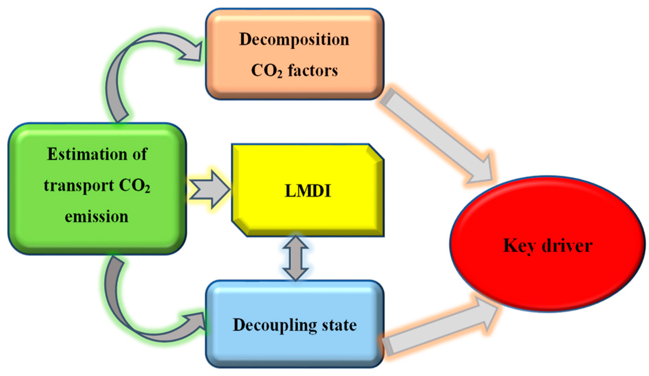
We drew a flow chart of modeling concepts and methodologies to demonstrate the modeling concepts clearly (Figure 1).

2.1.1. Transport Energy-Related CO₂ Emission Estimation

Energy-related CO₂ emissions from the transport industry can be calculated by the technique proposed by Intergovernmental Panel on Climate Change (IPCC) [49], the method is shown in Equation (1),

$$C=\sum \left(C_i\right)=\sum (E_i\ast {\alpha }_i\ast O_i\ast m)=\sum \left(E_i\ast C{F}_i\right)$$

(1)

where C_i (million tons CO₂ emission, Mt C) and E_i (million tons of coal equivalent, Mtce) denote the carbon emission and energy consumption of fuel. i, ${\alpha }_i$, and $O_i$ represent the standard carbon emission factor coefficient and the oxidation rate of fuel i; m is a constant with the numerical value of 44/12 (the molecular weight of CO₂ divided by the atomic weight of the element carbon). CF_i is CO₂ emission coefficient, and the value of each fuel used in this paper were shown in

Table 2. The carbon emission coefficient from fuel consumption in China.

Fuel Type	Coal	Oil	Gas
Emission coefficient (unit: Mt C/Mtce)	0.7476	0.5825	0.4435

Source: National Development and Reform Commission (NDRC) [50] and Chinese Academic Sciences [51].

. In this research, coal, oil, and natural gas were considered as three kinds of fuels and the energy consumption has been converted to million tons coal equivalent (Mtce).

2.1.2. Transport Decoupling Indices

Kaya [23] originally proposed multiplicative identities from population, gross domestic product (GDP) per capita (GDP/population), energy intensity (energy consumption/GDP), and CO₂ emission coefficient (CO₂ emission/energy consumption). Based on this decomposition method, we extend the original model to improve its pertinence for discussing transport-related CO₂ emission and the possibility of its decoupling from transport turnover volume. The possible influencing factors from the perspective of the Chinese transport sector can be obtained, and the factors are shown in Equation (2).

$$\begin{array}{cc}\hfill \mathrm{C}=\sum (C_{ij})=& \sum \left[\left(\frac{C_i}{E_i}\right)\ast \left(\frac{E_i}{E}\right)\ast \left(\frac{E}{N}\right)\ast \left(\frac{N}{N_j}\right)\ast \left(\frac{N_j}{T{V}_j}\right)\ast \left(\frac{T{V}_j}{TV}\right)\ast TV\right]\hfill \\ & =\sum \left(E{C}_i\ast E{M}_i\ast TE\ast T{S}_j\ast T{U}_j\ast T{M}_j\ast TV\right)\hfill \end{array}$$

(2)

E (Mtce) and N denote the energy consumption and the amount of the transport facilities; N_j and TV_j (ton-km, moving one ton of goods 1 km) represent the amount of transport and the turnover volume of the transport mode j. EC_i (CO₂ emission coefficient, $\frac{C_i}{E_i}$, Mt C/Mtce) and EM_i (transport energy mix, $\frac{E_i}{E}$, %) (i = 1, 2, 3 measures fuel coal, oil and gas) denote the carbon emission coefficient of fuel i and the energy mix of the transport energy consumption, respectively. TE (transport efficiency, $\frac{E}{N}$, Mtce/per unit) can be defined as the energy consumption in the transport sector divided by the total amount of transportation, revealing the transport efficiency; TS_j (transport share, $\frac{N}{N_j}$, %) uncovers the transport share of the transport mode j (j = 1,2,3,4 stands for the mode of railways, airways waterways and highways); TU_j (transportation facility usage, $\frac{N_j}{T{V}_j}$, units/ton-km) shows the transportation facility usage with per transport turnover volume added in a specific mode. TM_j (transport turnover mix, $\frac{T{V}_j}{TV}$, %) is the turnover mix of transport sector and TV (ton-km) denotes the transport turnover volume and the output of the transport sector, respectively.

It should be noted that the transport turnover volume in this paper is measured by the unit of ton-km. The passenger turnover unit of passenger-trip has been converted into the freight measurement of ton-km. By applying Equation (3), the passenger turnover volume can be converted. According to Zhang et al. [42], the conversion coefficient we used is shown in

Table 3. The conversion coefficient of turnover volume to ton-km.

Transport Mode	Highways	Railways	Waterways	Airways
Conversion coefficient	5	1	3.03	13.88

.

$$T{V}_j=\frac{T{V}_{j,1}}{CO}+T{V}_{j,2}$$

(3)

where $T{V}_{j,1}$ (per person–km, moving one person 1 km) and $T{V}_{j,2}$ (ton-km) denote the transport turnover volume from the passenger and freight of mode j; $CO$ stands for the conversion coefficient of turnover volume to ton-km.

To further quantify the contribution of each influencing factor to CO₂ emission decoupling from transport turnover volume, the decoupling index can be advanced by combining with the traditional logarithmic-mean Divisia index (LMDI) technique. Since the emission coefficient effect is considered stable, the corresponding carbon emission changes brought from other effects can then be interpreted as the energy mix effect ($E{M}_{effect}$), transport energy efficiency effect ($T{E}_{effect}$), transport facility share effect ($T{S}_{effect}$), transport usage effect ($T{U}_{effect}$), transport turnover mix effect ($T{M}_{effect}$), and transport turnover volume effect ($T{V}_{effect}$), these represent corresponding transport-related CO₂ emission changes from different factors.

We combine the potential factors that have been decomposed and the decoupling method proposed by Diakoulaki and Mandaraka [13] to detect the main drivers of decoupling status.

First, the total inhibition of CO₂ emission increase is shown in the equation:

$$\begin{array}{cc}\hfill \tau \left(C,TV\right)=& ∆C-T{V}_{effect}\hfill \\ & =E{M}_{effect}+T{E}_{effect}+T{S}_{effect}+T{U}_{effect}+T{M}_{effect}\hfill \end{array}$$

(4)

When $T{V}_{effect}>0$, the index of carbon emission decoupling from transport turnover volume can be defined as:

$$\begin{array}{cc}\hfill \mathsf{\beta }\left(C,TV\right)=& -\frac{\tau \left(C,TV\right)}{T{V}_{effect}}=-\frac{E{M}_{effect}}{T{V}_{effect}}-\frac{T{E}_{effect}}{T{V}_{effect}}-\frac{T{S}_{effect}}{T{V}_{effect}}-\frac{T{U}_{effect}}{T{V}_{effect}}-\frac{T{M}_{effect}}{T{V}_{effect}}\hfill \\ & ={\mathsf{\beta }}_{E{M}_{effect}}+{\mathsf{\beta }}_{T{E}_{effect}}+{\mathsf{\beta }}_{T{S}_{effect}}+{\mathsf{\beta }}_{T{U}_{effect}}+{\mathsf{\beta }}_{T{M}_{effect}}\hfill \end{array}$$

(5)

$\mathsf{\beta }\left(C,TV\right)$ denotes the index of carbon emission decoupling from transport turnover volume, ${\mathsf{\beta }}_{E{M}_{effect}}$, ${\mathsf{\beta }}_{T{E}_{effect}}$, ${\mathsf{\beta }}_{T{S}_{effect}}$, ${\mathsf{\beta }}_{T{U}_{effect}}$ and ${\mathsf{\beta }}_{T{M}_{effect}}$ were the contributions to the whole decoupling process from the energy mix effect, transport efficiency effect, transport share effect, transport usage effect, transport mix effect, and transport turnover volume effect.

However, in the case of the transport turnover volume factor having a negative impact on carbon emission increase, when $T{V}_{effect}<0$, the index can be interpreted as:

$$\begin{array}{cc}\hfill \mathsf{\beta }\left(C,TV\right)=& \frac{\tau \left(C,TV\right)-T{V}_{effect}}{T{V}_{effect}}\hfill \\ & =\frac{E{M}_{effect}-T{V}_{effect}}{T{V}_{effect}}+\frac{T{E}_{effect}-T{V}_{effect}}{T{V}_{effect}}+\frac{T{S}_{effect}-T{V}_{effect}}{T{V}_{effect}}\hfill \\ & +\frac{T{U}_{effect}-T{V}_{effect}}{T{V}_{effect}}+\frac{T{M}_{effect}-T{V}_{effect}}{T{V}_{effect}}+k\hfill \\ & ={\mathsf{\beta }}_{E{M}_{effect}}+{\mathsf{\beta }}_{T{E}_{effect}}+{\mathsf{\beta }}_{T{S}_{effect}}+{\mathsf{\beta }}_{T{U}_{effect}}+{\mathsf{\beta }}_{T{M}_{effect}}+k\hfill \end{array}$$

(6)

where k is a constant (k = 4). When $\mathsf{\beta }\left(C,TV\right)>1$, it can be defined as a strong decoupling state, with the curbing effects being effective at cutting carbon emissions, and with the effect being even more powerful than the CO₂ emission resulting from the transport output gains.

If $0<\mathsf{\beta }\left(C,TV\right)<1$, a relative decoupling state is found. Human efforts on CO₂ emission mitigation has some impact on actual CO₂ emission reduction, but the CO₂ emissions reduction effect is still weaker than the driving effect. In this state, the mitigation strategies have worked and cut down transport-related CO₂ emissions to some degree, while the curbing effects are still not as powerful as the CO₂ emissions resulting from the transport output gains.

In addition, when $\mathsf{\beta }\left(C,TV\right)<0$, no decoupling can be tested, CO₂ emission increase is in sync with transport output gains. The expected inhibiting factors do not reduce CO₂ emissions in the supposed way. In other words, the CO₂ emission from the expected curbing effects and the transport turnover volume both grew. Some of the promising inhabiting indictors did not work as effectively as expected. The specific effect that did not manage the target can then be determined by combining the decomposition technique after identifying ${\mathsf{\beta }}_{E{M}_{effect}}$, ${\mathsf{\beta }}_{T{E}_{effect}}$, ${\mathsf{\beta }}_{T{S}_{effect}}$, ${\mathsf{\beta }}_{T{U}_{effect}}$, and ${\mathsf{\beta }}_{T{M}_{effect}}$.

Based on the LMDI model [52] and the modified model [53], to calculate the weight coefficient, we decompose the transport-related CO₂ emission and calculate the CO₂ emission changes of each influencing factor. The CO₂ emission changes from the base year (the first of a series of years, year 0) to the target year (the last one of a series of years, year t) caused from each effect can be calculated by the LMDI technique, as shown in Equations (7)–(13):

$$E{M}_{effect}={\displaystyle \sum _{i=1}^3}\mu \left(C_i^t,C_i^0\right)\ast ln\left(\frac{E{M}^t}{E{M}^0}\right)$$

(7)

$$T{E}_{effect}={\displaystyle \sum _{i=1}^3}\mu \left(C_i^t,C_i^0\right)\ast ln\left(\frac{T{E}^t}{T{E}^0}\right)$$

(8)

$$\begin{array}{cc}\hfill T{S}_{effect}=& {\displaystyle \sum _{i=1}^3}\mu \left(C_i^t,C_i^0\right)\ast {\displaystyle \sum _{j=1}^4}\ln \left(\frac{T{S}_j^t}{T{S}_j^0}\right)\hfill \\ & =T{S}_{effect,railways}+T{S}_{effect,highways}+T{S}_{effect,waterways}+T{S}_{effect,airways}\hfill \\ & ={\displaystyle \sum _{i=1}^3}\mu \left(C_i^t,C_i^0\right)\ast \ln \left(\frac{T{S}_{j=1}^t}{T{S}_{j=1}^0}\right)+{\displaystyle \sum _{i=1}^3}\mu \left(C_i^t,C_i^0\right)\ast \ln \left(\frac{T{S}_{j=2}^t}{T{S}_{j=2}^0}\right)\hfill \\ & +{\displaystyle \sum _{i=1}^3}\mu \left(C_i^t,C_i^0\right)\ast \ln \left(\frac{T{S}_{j=3}^t}{T{S}_{j=3}^0}\right)+{\displaystyle \sum _{i=1}^3}\mu \left(C_i^t,C_i^0\right)\ast ln\left(\frac{T{S}_{j=4}^t}{T{S}_{j=4}^0}\right)\hfill \end{array}$$

(9)

$$\begin{array}{c}T{U}_{effect}={\displaystyle \sum _{i=1}^3}\mu \left(C_i^t,C_i^0\right)\ast {\displaystyle \sum _{j=1}^4}\ln \left(\frac{T{U}_j^t}{T{U}_j^0}\right)\hfill \\ =T{U}_{effect,railways}+T{U}_{effect,highways}+T{U}_{effect,waterways}+T{U}_{effect,airways}\hfill \\ ={\displaystyle \sum _{i=1}^3}\mu \left(C_i^t,C_i^0\right)\ast \ln \left(\frac{T{U}_{j=1}^t}{T{U}_{j=1}^0}\right)+{\displaystyle \sum _{i=1}^3}\mu \left(C_i^t,C_i^0\right)\ast \ln \left(\frac{T{U}_{j=2}^t}{T{U}_{j=2}^0}\right)\hfill \\ +{\displaystyle \sum _{i=1}^3}\mu \left(C_i^t,C_i^0\right)\ast \ln \left(\frac{T{U}_{j=3}^t}{T{U}_{j=3}^0}\right)+{\displaystyle \sum _{i=1}^3}\mu \left(C_i^t,C_i^0\right)\ast ln\left(\frac{T{U}_{j=4}^t}{T{U}_{j=4}^0}\right)\hfill \end{array}$$

(10)

$$\begin{array}{c}T{M}_{effect}={\sum }_{i=1}^3\mu \left(C_i^t,C_i^0\right)\ast {\sum }_{j=1}^{4}ln\left(\frac{T{M}_j^t}{T{M}_j^0}\right)\\ =T{M}_{effect,railways}+T{M}_{effect,highways}+T{M}_{effect,waterways}+T{M}_{effect,airways}\\ ={\displaystyle \sum _{i=1}^3}\mu \left(C_i^t,C_i^0\right)\ast \ln \left(\frac{T{M}_{j=1}^t}{T{M}_{j=1}^0}\right)+{\displaystyle \sum _{i=1}^3}\mu \left(C_i^t,C_i^0\right)\ast \ln \left(\frac{T{M}_{j=2}^t}{T{M}_{j=2}^0}\right)\\ +{\displaystyle \sum _{i=1}^3}\mu \left(C_i^t,C_i^0\right)\ast ln\left(\frac{T{M}_{j=3}^t}{T{M}_{j=3}^0}\right)+{\displaystyle \sum _{i=1}^3}\mu \left(C_i^t,C_i^0\right)\ast ln\left(\frac{T{M}_{j=4}^t}{T{M}_{j=4}^0}\right)\end{array}$$

(11)

$$T{V}_{effect}={\displaystyle \sum _{i=1}^3}\mu \left(C_i^t,C_i^0\right)\ast ln\left(\frac{T{V}^t}{T{V}^0}\right)$$

(12)

where the weight coefficient $\mu \left(C_i^t,C_i^0\right)$,

$$\mu \left(C_i^t,C_i^0\right)=\{\begin{array}{cc}\frac{C_i^t-C_i^0}{\ln C_i^t-\ln C_i^0},& C_i^t\ne C_i^{0}and{C}_i^t{C}_i^0\ne 0\\ C_i^0,& C_i^t=C_i^0\\ 0,& C_i^t{C}_i^0=0\end{array}$$

(13)

$C_i^t$ and $C_i^0$ denote CO₂ emission of fuel i of year 0 and year t. $E{M}_{effect}$ and $T{E}_{effect}$ denote CO₂ emission changes from the impacts of energy mix and transport efficiency;$T{S}_{effect}$, $T{U}_{effect}$, $T{M}_{effect}$, and $T{V}_{effect}$ represent the contributions of the transport facility share, transport usage, transport turnover mix, and transport turnover volume effects to transport-related CO₂ emission changes. It should be noted that the CO₂ emission changes from the transport share effect, transport usage of per transport turnover volume, and the transport mix variation were also identified from each transport mode (railways, airways, waterways, and highways).

2.2. Data Management

The transport energy consumption data of each fuel used in the paper was derived from the energy balance tables of the Chinese Energy Statistics Yearbook (CESY) [54] between 1990 and 2015. The fuel types included in this study were coal, oil, and gas; the carbon emission and energy consumption data were converted into the standard coal equivalent referring to the standard coal coefficients shown in CESY. Note that the energy consumption of transport, storage posts, and telecommunications industries was seen as a whole industry, and the share of the storage posts and telecommunications industry’s energy consumption was comparatively small (7.6% in 2007) [55], the energy use of all the stated industries were approximately considered as the energy consumption from the transport sector in this paper. The amount of transport facilities in different modes, the turnover volume of passengers and freight, were obtained from Chinese Statistics Yearbook [56] and the Transport Industry Development Statistics Bulletin [57].

3. Results

3.1. CO₂ Emission from Transport Sector

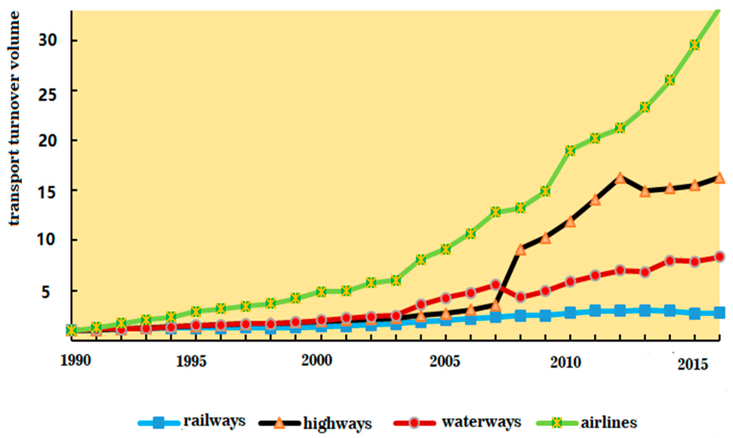
The CO₂ emission from transport was on the rise overall, increasing with an average annual rate of 6.65% in the last decade (2005–2015). Besides, CO₂ emission growth has been accelerating since 1995. What’s more, the emission changes have stepped into a new stage with a sharper increase after 2003. The turnover volume of each mode showed a growing trend despite some fluctuations. In general, air transport (green line) boomed with the highest change rate, whose average growth rate is 15.06% yr⁻¹, followed by road passengers and haulage (black line). In contrast, railways performed more stably than other transport modes, the turnover volume of railways only increased 4.13% per year. For airways, the turnover volume has grown over 33 times compared to the base year in 1990, indicating a huge improvement in the aviation travel mode. Also, for road travel in China, a sixteen-fold increase in the turnover ability has occurred since 1990.

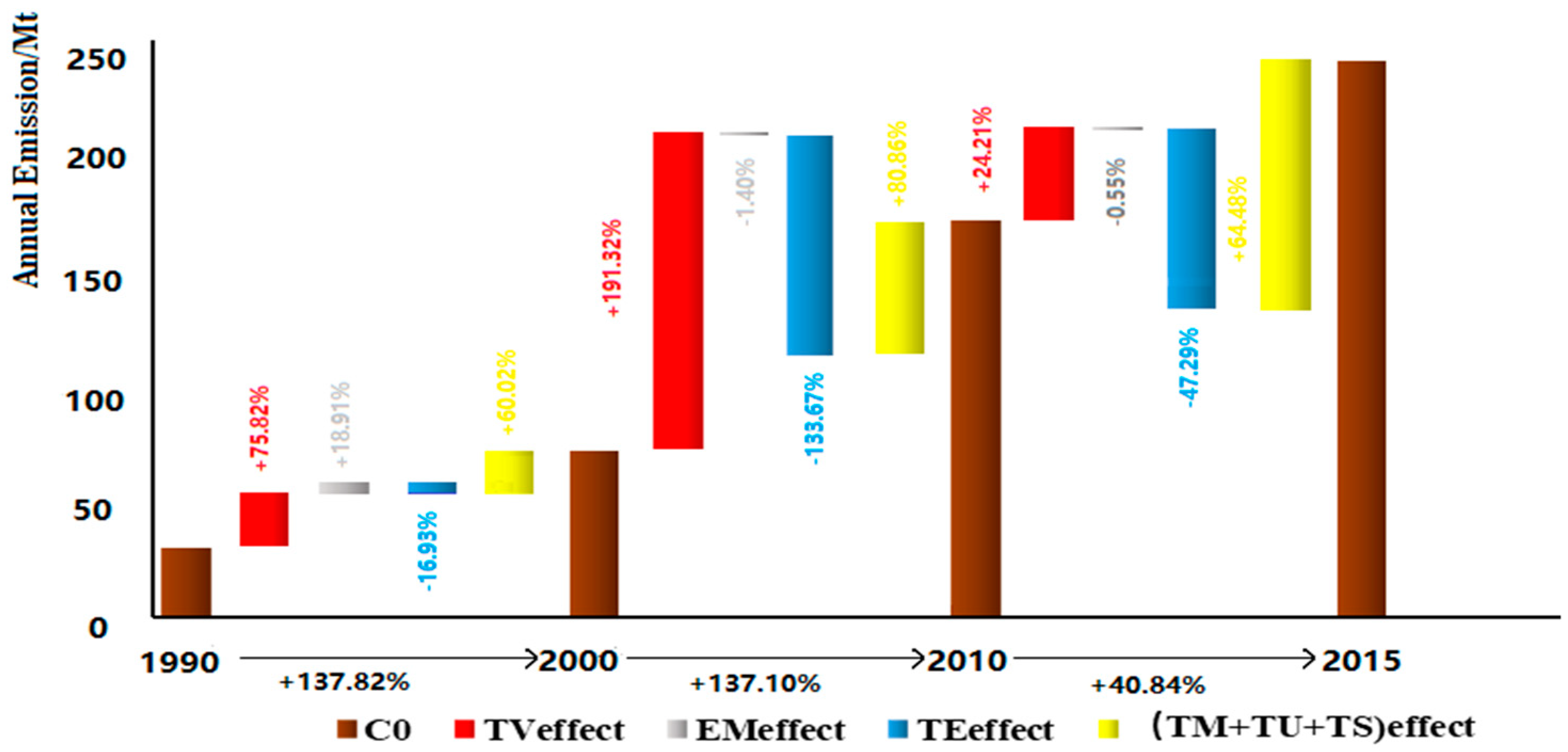
As shown in Figure 2, in general, the transport turnover volume effect contributed most to the increase in transport carbon emission of 75.82%, while the transport efficiency effect decreased the emission between 1990 and 2000. In the next decade, apart from energy mix changes, the other influencing factors showed more significant impacts on carbon emission, for instance, the transport efficiency effect cut 133.67% carbon emission, a great improvement compared to 16.93% in the first ten years. Relatively, the energy mix effect had minor influence on emission changes. To be more concrete, massive policy implementation on this issue may not achieve the desired effect to reduce carbon emission in the short term due to the transport efficiency improvement. The collective effect from transport share, transport usage, and transport dropped from 80.86% to 64.48%, however, since the total growth in CO₂ emission declined to 40.84%, the collective effect was still quite significant.

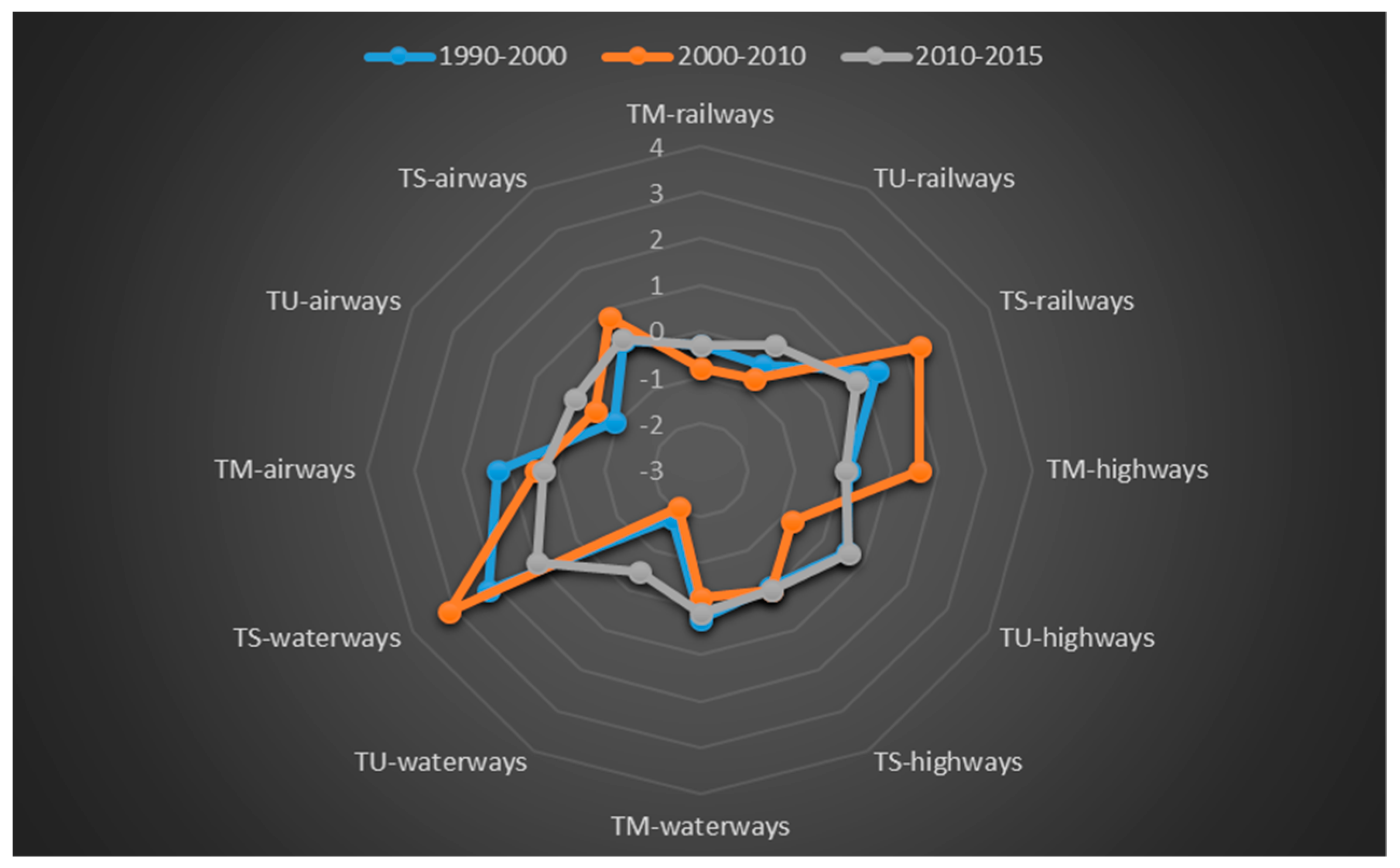
Apart from the overall contributions of the three effects, the specific impact of these three effects in different modes had been considered and the results are exhibited in Figure 3. For railways, both transport usage and transport mix cut down the carbon emission. 30.79% and 38.31% of the total CO₂ emission changes in the first ten years were from the railways turnover volume and the number of transport locomotives. Meanwhile, the locomotive proportion of the total transport system also brought about a decrease in carbon emission. Even though 1272 more railway locomotives were put into use in railway transport, the share of the total transport facilities dropped. However, the transport mix effect showed the most significant changes to water carriage in 1990–2000, 24.06% of the increased total CO₂ emission. Also, in the first phase, the transport facilities share effect of waterways caused 216.63% of the CO₂ emission, more than double the total carbon emission changes.

3.2. Driver Analysis of the Transport Decoupling Index

Overall, despite the mode differences, a weak decoupling state appeared between 1990–1995 and 2000–2010, offering empirical evidence for the decoupling of transport carbon emission from transport output. The decoupling index indicated the transport energy efficiency factor stimulated the decoupling in the observed period. The energy use of transport dropped 4.61% yr⁻¹, and after the year 2000, it decreased with the annual rate of 7.02%, indicating the improvement of energy use efficiency in the transport sector. Energy mix helped the decoupling. This may be because the popularity of transport motivated by renewable sources, such as electric cars, slowed down the transport carbon emission growth. To obtain further knowledge of the decoupling contribution from each indictor, an analysis was carried out in consideration of the character identification of different transport modes and the results are shown in

Table 4. The decoupling index and impacts from various factors of railways.

Year	${\mathsf{\beta }}_{\mathit{T}{\mathit{M}}_{\mathit{r}\mathit{a}\mathit{i}\mathit{l}\mathit{w}\mathit{a}\mathit{y}\mathit{s}}}$	${\mathsf{\beta }}_{\mathit{T}{\mathit{U}}_{\mathit{r}\mathit{a}\mathit{i}\mathit{l}\mathit{w}\mathit{a}\mathit{y}\mathit{s}}}$	${\mathsf{\beta }}_{\mathit{T}{\mathit{S}}_{\mathit{r}\mathit{a}\mathit{i}\mathit{l}\mathit{w}\mathit{a}\mathit{y}\mathit{s}}}$	${\mathsf{\beta }}_{\mathit{E}{\mathit{M}}_{\mathit{e}\mathit{f}\mathit{f}\mathit{e}\mathit{c}\mathit{t}}}$	${\mathsf{\beta }}_{\mathit{T}{\mathit{E}}_{\mathit{e}\mathit{f}\mathit{f}\mathit{e}\mathit{c}\mathit{t}}}$	β	State
1990–1995	0.14	−0.03	−0.20	−0.08	0.17	0.48	relative decoupling
1995–2000	0.10	0.37	−0.52	−0.82	0.19	−2.03	no decoupling
2000–2005	0.14	0.09	−0.28	−0.03	0.18	0.08	relative decoupling
2005–2010	0.10	0.14	−0.38	0.02	0.23	0.42	relative decoupling
2010–2015	0.38	−0.44	−0.64	0.00	0.32	−0.69	no decoupling

,

Table 5. The decoupling index and impacts from various factors of road transport.

Year	${\mathsf{\beta }}_{\mathit{T}{\mathit{M}}_{\mathit{h}\mathit{i}\mathit{g}\mathit{h}\mathit{w}\mathit{a}\mathit{y}\mathit{s}}}$	${\mathsf{\beta }}_{\mathit{T}{\mathit{U}}_{\mathit{h}\mathit{i}\mathit{g}\mathit{h}\mathit{w}\mathit{a}\mathit{y}\mathit{s}}}$	${\mathsf{\beta }}_{\mathit{T}{\mathit{S}}_{\mathit{h}\mathit{i}\mathit{g}\mathit{h}\mathit{w}\mathit{a}\mathit{y}\mathit{s}}}$	${\mathsf{\beta }}_{\mathit{E}{\mathit{M}}_{\mathit{e}\mathit{f}\mathit{f}\mathit{e}\mathit{c}\mathit{t}}}$	${\mathsf{\beta }}_{\mathit{T}{\mathit{E}}_{\mathit{e}\mathit{f}\mathit{f}\mathit{e}\mathit{c}\mathit{t}}}$	β	State
1990–1995	0.04	−0.15	0.01	−0.08	0.17	0.48	relative decoupling
1995–2000	0.11	−0.18	0.01	−0.82	0.19	−2.03	no decoupling
2000–2005	0.08	−0.14	0.00	−0.03	0.18	0.08	relative decoupling
2005–2010	−0.01	−0.13	0.00	0.02	0.23	0.42	relative decoupling
2010–2015	−0.19	−0.52	0.00	0.00	0.32	−0.69	no decoupling

and

Table 6. The decoupling index and impacts from various factors of water transport.

Year	${\mathsf{\beta }}_{\mathit{T}{\mathit{M}}_{\mathit{w}\mathit{a}\mathit{t}\mathit{e}\mathit{r}\mathit{w}\mathit{a}\mathit{y}\mathit{s}}}$	${\mathsf{\beta }}_{\mathit{T}{\mathit{U}}_{\mathit{w}\mathit{a}\mathit{t}\mathit{e}\mathit{r}\mathit{w}\mathit{a}\mathit{y}\mathit{s}}}$	${\mathsf{\beta }}_{\mathit{T}{\mathit{S}}_{\mathit{w}\mathit{a}\mathit{t}\mathit{e}\mathit{r}\mathit{w}\mathit{a}\mathit{y}\mathit{s}}}$	${\mathsf{\beta }}_{\mathit{E}{\mathit{M}}_{\mathit{e}\mathit{f}\mathit{f}\mathit{e}\mathit{c}\mathit{t}}}$	${\mathsf{\beta }}_{\mathit{T}{\mathit{E}}_{\mathit{e}\mathit{f}\mathit{f}\mathit{e}\mathit{c}\mathit{t}}}$	β	State
1990–1995	−0.15	0.31	−0.26	−0.08	0.17	0.48	relative decoupling
1995–2000	−0.11	0.88	−0.83	−0.82	0.19	−2.03	no decoupling
2000–2005	−0.10	0.42	−0.37	−0.03	0.18	0.08	relative decoupling
2005–2010	−0.05	0.33	−0.41	0.02	0.23	0.42	relative decoupling
2010–2015	−0.03	0.14	−0.82	0.00	0.32	−0.69	no decoupling

.

3.2.1. Decoupling for Railways

For railways, transport turnover mix accelerated the decoupling process and the increasingly active role of the transport turnover mix effect raised the likelihood of decoupling. Since the railways share of the total transport is the reciprocal of $TS$, after calculating the value of ${\mathsf{\beta }}_{T{S}_{railways}}$, the drop of railways locomotives’ share was found to hinder the carbon emission decoupling from transport output gains. That is to say, as a low carbon emission travel mode, reducing the share of railway facilities can slow down the decoupling process. This indicates that apart from the transport energy efficiency effect accelerating the decoupling of carbon emission from transport output, for railways, the turnover ability accelerated the transport-related CO₂ emission decoupling from turnover volume added. However, since the railway transport turnover volume did not compete with the growing speed of the total transport industry output, the turnover capacity should be further improved.

3.2.2. Decoupling for Road Transport

As shown in Table 5, the decoupling index of the transport turnover mix effect uncovered that changes of the mix impeded the decoupling trend after 2005, however, the turnover volume share of road transport grew from 12.09% to 31.91% (Figure 4). Compared to an annual drop of 0.72%, the sharp increase of 10.19% yr⁻¹ hindered the decoupling process.

${\mathsf{\beta }}_{T{U}_{highways}}$ was negative through all twenty-five years, indicating that vehicle usage efficiency was limited to a relatively low level and the situation has not been improved yet in the observed period. However, since more private cars were put into use and the number might be on the rise for a period, more research on the technology improvement related to vehicle usage efficiency is needed. In addition, the vehicle proportion of the total transport system increased while the carbon emission dropped. This may attributable to the widespread use of new electric vehicles as private cars and city buses.

3.2.3. Decoupling for Waterways

The decoupling index of the water transport turnover mix, as demonstrated in Table 6, curbed the decoupling process, indicating that the turnover volume from waterways was still at a low level in China. The decoupling of transport usage revealed that waterways efficiency in China contributed to decoupling. The transport usage effect for water travel provided impetus for decoupling evolution, indicating that the water transport efficiency in China was positively related to the decoupling of transport carbon emission and turnover volume. According to ${\mathsf{\beta }}_{T{S}_{waterways}}$, the transport facilities share effect of water travel hindered the decoupling process. In this case, the waterways facilities proportion of the whole transport facilities promoted the carbon emission decoupling from turnover in reverse. In other words, more ships or other water travel facilities usage within an acceptable price range can accelerate the decoupling. Therefore, a switch from high emission modes of transport to low emission modes, such as road transport to waterways, can boost transport–emission decoupling in China to some degree.

3.2.4. Decoupling for Airways

As is shown in

Table 7. The decoupling index and impacts from various factors of air transport.

Year	${\mathsf{\beta }}_{\mathit{T}{\mathit{M}}_{\mathit{a}\mathit{i}\mathit{r}\mathit{w}\mathit{a}\mathit{y}\mathit{s}}}$	${\mathsf{\beta }}_{\mathit{T}{\mathit{U}}_{\mathit{a}\mathit{i}\mathit{r}\mathit{w}\mathit{a}\mathit{y}\mathit{s}}}$	${\mathsf{\beta }}_{\mathit{T}{\mathit{S}}_{\mathit{a}\mathit{i}\mathit{r}\mathit{w}\mathit{a}\mathit{y}\mathit{s}}}$	${\mathsf{\beta }}_{\mathit{E}{\mathit{M}}_{\mathit{e}\mathit{f}\mathit{f}\mathit{e}\mathit{c}\mathit{t}}}$	${\mathsf{\beta }}_{\mathit{T}{\mathit{E}}_{\mathit{e}\mathit{f}\mathit{f}\mathit{e}\mathit{c}\mathit{t}}}$	$\mathsf{\beta }$	State
1990–1995	−0.43	0.56	−0.22	−0.08	0.17	0.48	relative decoupling
1995–2000	−0.30	0.60	−0.36	−0.82	0.19	−2.03	no decoupling
2000–2005	0.03	−0.03	−0.05	−0.03	0.18	0.08	relative decoupling
2005–2010	−0.19	0.24	−0.19	0.02	0.23	0.42	relative decoupling
2010–2015	9.40	−1.12	−0.16	0.05	−3.65	−0.69	no decoupling

, since ${\mathsf{\beta }}_{T{S}_{airways}}<0$, the transport facilities share effect of airways resembled the waterways, exerting a negative impact on decoupling evolution. With the expansion of air transport facilities, the decoupling process will accelerate. However, since air transport is considered a relatively carbon-intensive mode and the second largest emitter to the whole transport modes [17], the efficiency of air transport should be improved. Even though the turnover mix of air transport and transport usage effect had a distinct impact on the decoupling trend in different stages, the turnover volume of air transport increased greatly compared with other modes, especially after 2003 (shown in Figure 4). Overall, the number of aircraft per unit transport output added rose by 6.41% from 2010 to 2015. The decoupling index of the air transport usage effect had a negative effect during this period. Future mitigation or decoupling strategies can focus on technology improvement such as energy usage improvement.

4. Discussion

In addition to focusing on economic issues, developing relevant strategies from the perspective of the transport sector, such as transport energy efficiency improvement [58], can be feasible for policy makers to break the rigid link between transport-related CO₂ emission and transport output. According to the results, the transport energy mix effect primarily contributed to the decoupling process in China’s transport sector, which is consistent with Dhar and Marpaung’s study on Asia’s transport-related CO₂ emissions [59]. When decomposing, unlike most previous studies aimed at discussing influencing factors, such as population, GDP per capita, energy intensity, and emission coefficient effects, we focused more on identifying the causes from within the transportation sector. In this way, it is beneficial for the government to develop more pertinent and feasible strategies to cut down the CO₂ emissions of the transport sector. After analyzing the contributions of each factor to transport-related CO₂ emission changes, the transport turnover volume effect was found to be the most significant factor increasing transport-related CO₂ emissions in the observed period in China. Meanwhile, the transport efficiency effect contributed to cutting down transport-related CO₂ emissions, where a key element is the improvement and renovation of mitigation and energy conversion technologies. Similarly, according to Edelenbosch et al. [41], technology transition is overwhelmingly needed.

Previous decoupling studies on traffic carbon emissions primarily concentrated on the correlation analysis of CO₂ emissions and economic value added. The decoupling status of transport-related CO₂ emissions and economic growth has also been found [60,61]. However, because of the accelerating transport-related CO₂ emissions in China, the exploration of feasible measures is in desperate need. In order to reduce transport-related CO₂ emissions more effectively, pertinent mitigation strategies of the transport sector are needed, not just economic or social aspects. The relative decoupling state appeared between 1990–1995 and 2000–2010, revealing the possibility of decoupling transport-related CO₂ emission from turnover volume.

Moreover, most of the studies on decoupling focus on analyzing decoupling states, and few have investigated the contribution of various factors that cause this decoupling state. But, to achieve a decoupling state now, or a possible strong decoupling state in the future, the real reason of the related decoupling states is of vital importance.

So, after testing the decoupling state in different phases, we quantified the factors’ contributions to the decoupling process. Overall, railway transport was a sector with a comparatively high level of turnover capacity compared to other transport modes. After decomposing the main drivers of CO₂ emissions increase from passenger cars in Greece and Denmark, a close connection between vehicle ownership and CO₂ emissions was detected [37]. In our research, the transport usage effect of road transport and the vehicle proportion of all the transport facilities impeded the decoupling process, which is consistent.

According to Ang [20], the LMDI (logarithmic-mean Divisia index) method we used in this research is considered to be a preferred approach because of its ease of use and adaptability. Also, unlike the hypotheses or ideal conditions that must be made before applying econometric models, the LMDI method can be adapted with no strict prerequisites. Yet, there are some questions we cannot address thoroughly at the moment. Not all the possible factors can be analyzed due to the limit of the Kaya identity (must be divided into several multiplications). We can only select the main factors to carry out our research on the basis of a detailed review of the previous studies related to the same topic. In future work, we will deepen our research by considering more spatial issues, such as spatially stratified heterogeneity. To achieve the ultimate goal of sustainability in the transport sector, technology improvement and switching are currently considered significant and effective measures.

5. Conclusions and Policy Implications

This paper chose China as an empirical case to analyze the decoupling possibility of transport-related CO₂ emissions from transport turnover volume. The transport decoupling states of different travel modes in China were identified from the perspective of each mode’s characteristics and the decoupling decomposition analyses were carried out, respectively. In brief, some conclusions and relevant policy implications to promote the decoupling evolution are stated:

Transport-related CO₂ emissions have increased and carbon emission growth has accelerated since 1995. Among all the drivers, the transport turnover volume effect was the primary driver of carbon emission growth in the transport industry in China, while the transport efficiency effect cut down the transport-related CO₂ emissions. The technology of energy use in the transport industry should focus more on energy efficiency improvement. Also, with the rise in car ownership in recent years, developing strategies for changing passengers’ travelling behavior should be considered. For example, offering convenient and affordable public transit solutions. In general, the transport energy efficiency effect reduced the transport-related carbon emissions during the observed period. The railway turnover mix decreased carbon emissions, while road and air transport added more CO₂ emissions. Apart from the vehicle share of the transport facilities increasing the CO₂ emission, all the other travel modes put a brake on emission growth. Consequently, modal replacement strategies should be encouraged to foster CO₂ emission mitigation.

Relative decoupling states appeared between 1990–1995 and 2000–2010 in China, indicating the possibility that transport-related CO₂ emission decoupling from turnover volume gains is possible, giving empirical evidence for other countries. Overall, the transport energy efficiency effect contributed the most in advancing the transport-related CO₂ emission decoupling from turnover volume for all transport modes, while the energy mix effect hindered the decoupling process in most observed periods. Apart from road transport, the proportion of other travel modes’ growth can boost decoupling. The transport usage effect of road transport and the vehicle proportion of transport facilities impeded the decoupling process. Since the bike-sharing systems in China has been set up [62], the shared transport system of other travel modes can be explored. For the decoupling evolution, railway transport was a sector with a relatively high level of turnover capacity, advancing the railways carbon emission decoupling from all the transport industry output gains.

For railways, transport turnover mix and railways locomotives share rises can boost the decoupling evolution. Since the 1990s, rail-transport has been steadily replaced by vehicles in China. Locomotive ownership increased by 1.64% yr⁻¹, rather slow compared to 22.88% yr⁻¹ for private cars. Thus, revitalizing the railways within acceptable expenses should be considered. For instance, in addition to the continuous energy efficiency improvement, pouring more money to railway turnover technology innovations should be encouraged.

The changes of the vehicles turnover mix impeded the decoupling after 2005 in China. Because of the sharp rise of private cars, the decoupling has slowed. Since the private vehicles proportion of civil vehicles in China grew from 14.80% in 1990 to 87.92% in 2015, more incentives to encourage travel mode switching should be provided. Besides infrastructure improvement, price policies concerning road transport, such as levying more taxes on road maintenance, parking, or insurance should also be considered. What’s more, the “Smart Growth” development pattern [63] can be adopted, for example, the Bus Rapid Transit (BRT) system can be promoted further to replace current individual car-oriented travel choices.

The water transport turnover mix hindered the decoupling evolution, while the waterways transport usage effect stimulated transport-related CO₂ emission decoupling from turnover volume. Likewise, the rising proportion of waterways facilities promoted the carbon emission decoupling from turnover in China in the observed years. With the increase in air transport facilities proportion, the decoupling process from transport output will accelerate. The turnover mix of air transport and the transport usage effect had a distinct impact on the decoupling trend in different stages. According to Loo and Li [17], water transport can be a low carbon emission transport mode, whereas air transport is the second largest contributor to transport-related carbon emissions. Meanwhile, with the limits of funding and sustainable technology, policies should combine economic and environmental systems to achieve the decoupling goal.

References

- IEA. CO2 Emissions from Fuel Combustion; International Energy Agency: Paris, France, 2017. [Google Scholar]
- Wang, Q.; Chen, X. Energy policies for managing China’s carbon emission. Renew. Sust. Energ. Rev. 2015, 50, 470–479. [Google Scholar] [CrossRef]
- Wang, Q. China should aim for a total cap on emissions. Nature 2014, 512, 115. [Google Scholar] [CrossRef] [PubMed]
- Li, R.R.; Su, M. The role of natural gas and renewable energy in curbing carbon emission: Case study of the United States. Sustainability 2017, 9, 600. Available online: https://www.mdpi.com/2071-1050/9/4/600 (accessed on 15 August 2018). [CrossRef]
- Wang, Q.; Zhao, M.; Li, R.; Su, M. Decomposition and decoupling analysis of carbon emissions from economic growth: A comparative study of China and the United States of America. J. Clean. Prod. 2018, 197, 178–184. [Google Scholar] [CrossRef]
- Jiang, R.; Zhou, Y.; Li, R. Moving to a Low-Carbon Economy in China: Decoupling and Decomposition Analysis of Emission and Economy from a Sector Perspective. Sustainability 2018, 10, 978. Available online: www.mdpi.com/2071-1050/10/4/978/pdf (accessed on 15 August 2018). [CrossRef]
- Wang, Q.; Jiang, R.; Li, R. Decoupling analysis of economic growth from water use in City: A case study of Beijing, Shanghai, and Guangzhou of China. Sustain. Cities Soc. 2018, 41, 86–94. [Google Scholar] [CrossRef]
- Wang, Q.; Chen, X.; Yi-chong, X. Accident like the Fukushima unlikely in a country with effective nuclear regulation: Literature review and proposed guidelines. Renew. Sustain. Energy Rev. 2013, 17, 126–146. [Google Scholar] [CrossRef]
- Weizsäcker, E.U.V. Erdpolitik: Ökologische Realpolitik an der Schwelle zum Jahrhundert der Umwelt; Wissenschaftliche Buchgesellschaft: Darmstadt, Germany, 1990. [Google Scholar]
- Zhang, Z. Decoupling China’s Carbon Emissions Increase from Economic Growth: An Economic Analysis and Policy Implications. World Dev. 2000, 28, 739–752. [Google Scholar] [CrossRef]
- Ruefing, K. Indicators to Measure Decoupling of Environmental Pressure from Economic Growth; Island Press: Washington, DC, USA, 2007; pp. 211–222. [Google Scholar]
- Tapio, P. Towards a theory of decoupling: Degrees of decoupling in the EU and the case of road traffic in Finland between 1970 and 2001. Transp. Policy 2005, 12, 137–151. [Google Scholar] [CrossRef]
- Diakoulaki, D.; Mandaraka, M. Decomposition analysis for assessing the progress in decoupling industrial growth from CO2 emissions in the EU manufacturing sector. Energy Econ. 2007, 29, 636–664. [Google Scholar] [CrossRef]
- Loo, B.P.Y.; Banister, D. Decoupling transport from economic growth: Extending the debate to include environmental and social externalities. J. Transp. Geogr. 2016, 57, 134–144. [Google Scholar] [CrossRef]
- Alises, A.; Vassallo, J.M.; Guzmán, A.F. Road freight transport decoupling: A comparative analysis between the United Kingdom and Spain. Transp. Policy 2014, 32, 186–193. [Google Scholar] [CrossRef]
- He, K.; Huo, H.; Zhang, Q.; He, D.; An, F.; Wang, M.; Walsh, M.P. Oil consumption and CO2 emissions in China’s road transport: Current status, future trends, and policy implications. Energy Policy 2005, 33, 1499–1507. [Google Scholar] [CrossRef]
- Loo, B.P.Y.; Li, L. Carbon dioxide emissions from passenger transport in China since 1949: Implications for developing sustainable transport. Energy Policy 2012, 50, 464–476. [Google Scholar] [CrossRef]
- Wang, Q.; Jiang, X.-t.; Li, R. Comparative decoupling analysis of energy-related carbon emission from electric output of electricity sector in Shandong Province, China. Energy 2017, 127, 78–88. [Google Scholar] [CrossRef]
- Ang, B.W.; Goh, T. Bridging the gap between energy-to-GDP ratio and composite energy intensity index. Energy Policy 2018, 119, 105–112. [Google Scholar] [CrossRef]
- Ang, B.W. Decomposition analysis for policymaking in energy: Which is the preferred method? Energy Policy 2004, 32, 1131–1139. [Google Scholar] [CrossRef]
- Wang, Q.; Li, R. Journey to burning half of global coal: Trajectory and drivers of China’s coal use. Renew. Sustain. Energy Rev. 2016, 58, 341–346. [Google Scholar] [CrossRef]
- Ehrlich, P.R.; Holdren, J.P. Impact of Population Growth. Science 1971, 171, 1212. Available online: http://www.jstor.org/stable/1731166 (accessed on 17 August 2018). [CrossRef] [PubMed]
- Kaya, Y. Impact of Carbon Dioxide Emission Control on GNP Growth: Interpretation of Proposed Scenarios; Paper presented the IPCC Energy and Industry Subgroup; Response Strategies Working Group: Paris, France, 1990. [Google Scholar]
- Dietz, T.; Rosa, E.A. Rethinking the environmental impacts of population, Affluence and technology. Hum. Ecol. Rev. 1994, 1, 277–300. [Google Scholar] [CrossRef]
- Rose, A.; Casier, S. Input–Output Structural Decomposition Analysis: A Critical Appraisal. Econ. Syst. Res. 1996, 8, 33–62. [Google Scholar] [CrossRef]
- Dietz, T.; Rosa, E.A. Effects of Population and Affluence on CO2 Emissions. Proc. Natl. Acad. Sci. USA 1997, 94, 175–179. [Google Scholar] [CrossRef] [PubMed]
- Leontief, W. Environmental Repercussions and the Economic Structure: An Input-Output Approach. Rev. Econ. Stat. 1970, 56, 109–110. [Google Scholar] [CrossRef]
- Dietzenbacher, E.; Los, B. Structural Decomposition Techniques: Sense and Sensitivity. Econ. Syst. Res. 1998, 10, 307–324. [Google Scholar] [CrossRef]
- Su, B.; Ang, B.W. Structural decomposition analysis applied to energy and emissions: Some methodological developments. Energy Econ. 2012, 34, 177–188. [Google Scholar] [CrossRef]
- Liao, C.H.; Lu, C.S.; Tseng, P.H. Carbon dioxide emissions and inland container transport in Taiwan. J. Transp. Geogr. 2011, 19, 722–728. [Google Scholar] [CrossRef]
- Zhang, C.; Nian, J. Panel estimation for transport sector CO2 emissions and its affecting factors: A regional analysis in China. Energy Policy 2013, 63, 918–926. [Google Scholar] [CrossRef]
- Paravantis, J.A.; Georgakellos, D.A. Trends in energy consumption and carbon dioxide emissions of passenger cars and buses. Technol. Forecast. Soc. Chang. 2007, 74, 682–707. [Google Scholar] [CrossRef]
- Shakya, S.R.; Shrestha, R.M. Transport sector electrification in a hydropower resource rich developing country: Energy security, environmental and climate change co-benefits. Energy Sustain. Dev. 2011, 15, 147–159. [Google Scholar] [CrossRef]
- Graham, D.J.; Crotte, A.; Anderson, R.J. A dynamic panel analysis of urban metro demand. Transp. Res. Part E Logist. Transp. Rev. 2009, 45, 787–794. [Google Scholar] [CrossRef]
- Simões, A.F.; Schaeffer, R. The Brazilian air transportation sector in the context of global climate change: CO2 emissions and mitigation alternatives. Energy Convers. Manag. 2005, 46, 501–513. [Google Scholar] [CrossRef]
- Scholl, L.; Schipper, L.; Kiang, N. CO2 emissions from passenger transport: A comparison of international trends from 1973 to 1992. Energy Policy 1996, 24, 17–30. [Google Scholar] [CrossRef]
- Papagiannaki, K.; Diakoulaki, D. Decomposition analysis of CO2 emissions from passenger cars: The cases of Greece and Denmark. Energy Policy 2009, 37, 3259–3267. [Google Scholar] [CrossRef]
- Achour, H.; Belloumi, M. Decomposing the influencing factors of energy consumption in Tunisian transportation sector using the LMDI method. Transp. Policy 2016, 52, 64–71. [Google Scholar] [CrossRef]
- Feng, T.-T.; Yang, Y.-S.; Xie, S.-Y.; Dong, J.; Ding, L. Economic drivers of greenhouse gas emissions in China. Renew. Sustain. Energy Rev. 2017, 78, 996–1006. [Google Scholar] [CrossRef]
- Luo, X.; Dong, L.; Dou, Y.; Li, Y.; Liu, K.; Ren, J.; Liang, H.; Mai, X. Factor decomposition analysis and causal mechanism investigation on urban transport CO2 emissions: Comparative study on Shanghai and Tokyo. Energy Policy 2017, 107, 658–668. [Google Scholar] [CrossRef]
- Edelenbosch, O.Y.; McCollum, D.L.; van Vuuren, D.P.; Bertram, C.; Carrara, S.; Daly, H.; Fujimori, S.; Kitous, A.; Kyle, P.; Ó Broin, E.; et al. Decomposing passenger transport futures: Comparing results of global integrated assessment models. Transp. Res. Part D Transp. Environ. 2017, 55, 281–293. [Google Scholar] [CrossRef]
- Andrés, L.; Padilla, E. Driving factors of GHG emissions in the EU transport activity. Transp. Policy 2018, 61, 60–74. [Google Scholar] [CrossRef]
- Schipper, L.; Steiner, R.; Duerr, P.; An, F.; Strøm, S. Energy use in passenger transport in OECD countries: Changes since 1970. Transportation 1992, 19, 25–42. [Google Scholar] [CrossRef]
- Danielis, R. Energy use for transport in Italy: Past trends. Energy Policy 1995, 23, 799–807. [Google Scholar] [CrossRef]
- Kiang, N.; Schipper, L. Energy trends in the Japanese transportation sector. Transp. Policy 1996, 3, 21–35. [Google Scholar] [CrossRef]
- Greening, L.A.; Ting, M.; Davis, W.B. Decomposition of aggregate carbon intensity for freight: Trends from 10 OECD countries for the period 1971–1993. Energy Econ. 1999, 21, 331–361. [Google Scholar] [CrossRef]
- Kwon, T.-H. Decomposition of factors determining the trend of CO2 emissions from car travel in Great Britain (1970–2000). Ecol. Econ. 2005, 53, 261–275. [Google Scholar] [CrossRef]
- Sobrino, N.; Monzon, A. The impact of the economic crisis and policy actions on GHG emissions from road transport in Spain. Energy Policy 2014, 74, 486–498. [Google Scholar] [CrossRef] [Green Version]
- IPCC. Greenhouse Gas Inventory: IPCC Guidelines for National Greenhouse Gas Inventories; IPCC: Bracknell, UK, 2006. [Google Scholar]
- National Development and Reform Commission. China’s Sustainable Development Energy and Carbon Emission Scenarios. 2003. Available online: http://www.efchina.org/Attachments/Report/reports-efchina-20061209-6-zh/Fnl_Scenario_CN.pdf (accessed on 17 August 2018). (In Chinese).
- CAS Sustainable Development Strategy Team. China’s Sustainable Development Strategy Report in 2009; Science Press: Beijing, China, 2009. [Google Scholar]
- Ang, B.W.; Liu, F.L.; Chew, E.P. Perfect decomposition techniques in energy and environmental analysis. Energy Policy 2003, 31, 1561–1566. [Google Scholar] [CrossRef]
- Wang, Q.; Li, S.; Li, R.; Ma, M. Forecasting U.S. shale gas monthly production using a hybrid ARIMA and metabolic nonlinear grey model. Energy 2018, 160, 378–387. [Google Scholar] [CrossRef]
- National Bureau of Statistics. Chinese Energy Statistics Yearbook 2016; China Statistics Press: Beijing, China, 2016.
- Fan, F.; Lei, Y. Decomposition analysis of energy-related carbon emissions from the transportation sector in Beijing. Transp. Res. Part D Transp. Environ. 2016, 42, 135–145. [Google Scholar] [CrossRef]
- National Bureau of Statistics. Chinese Statistics Yearbook 2017; China Statistics Press: Beijing, China, 2017.
- Ministry of Transport of the People’s Republic of China: Transport Industry Development Statistics Bulletin (2015). 2016. Available online: http://zizhan.mot.gov.cn/zfxxgk/bnssj/zhghs/201605/t20160506_2024006.html (accessed on 17 August 2018). (In Chinese)
- Xu, B.; Lin, B. Carbon dioxide emissions reduction in China’s transport sector: A dynamic VAR (vector autoregression) approach. Energy 2015, 83, 486–495. [Google Scholar] [CrossRef]
- Dhar, S.; Marpaung, C.O.P. Technology priorities for transport in Asia: Assessment of economy-wide CO2 emissions reduction for Lebanon. Clim. Chang. 2015, 131, 451–464. [Google Scholar] [CrossRef] [Green Version]
- Roinioti, A.; Koroneos, C. The decomposition of CO2 emissions from energy use in Greece before and during the economic crisis and their decoupling from economic growth. Renew. Sustain. Energy Rev. 2017, 76, 448–459. [Google Scholar] [CrossRef]
- Wang, Y.; Xie, T.; Yang, S. Carbon emission and its decoupling research of transportation in Jiangsu Province. J. Clean. Prod. 2017, 142, 907–914. [Google Scholar] [CrossRef]
- The Guardian Uber for Bikes: How ‘Dockless’ Cycles Flooded China—And Are Heading Overseas. Available online: https://www.theguardian.com/cities/2017/mar/22/bike-wars-dockless-china-millions-bicycles-hangzhou (accessed on 11 April 2018).
- Houdashelt, M. Reducing Transportation Emissions: Travel Demand Measures; Center for Clean Air Policy: Paris, France, 2006. [Google Scholar]
Figure 1.
Flow chart of modeling concepts and methodologies.
Figure 2.
Annual transport-related carbon emission changes from different effects.
Figure 3.
The modal contribution differences for three periods.
Figure 4.
Trajectory of transport turnover volume of different modes. (All quantities were normalized to 1 at 1990)