How to Guarantee the Sustainability of the Wind Prevention and Sand Fixation Service: An Ecosystem Service Flow Perspective


1
Institute of Geographic Sciences and Natural Resources Research, Chinese Academy of Sciences, A11 Datun Road, Beijing 100101, China
2
College of Resources and Environment, University of Chinese Academy of Sciences, 19 A Yuquan Road, Shijingshan District, Beijing 100049, China
3
Faculty of Geographical Science, Beijing Normal University, No. 19, XinJieKouWai St., HaiDian District, Beijing 100875, China
*
Author to whom correspondence should be addressed.
Sustainability 2018, 10(9), 2995; https://doi.org/10.3390/su10092995
Submission received: 21 July 2018
/
Revised: 16 August 2018
/
Accepted: 21 August 2018
/
Published: 23 August 2018
Abstract
:Assessing ecosystem services (ESs) is essential for sustainable development. Ecosystem service flow (ESF) emphasizes the recognition of real ESs beneficiary areas from the perspective of human welfare and establishes a spatiotemporal path between service supply areas (SSAs) and service beneficiary areas (SBAs) to better reflect the relationship between ESs and human welfare, which is conducive to recognize how to guarantee the sustainable supply of ESs. This study simulated the spatiotemporal patterns and flow trajectories of the wind prevention and sand fixation (WPSF) service in Yanchi County based on the Revised Wind Erosion Equation (RWEQ) and the Hybrid Single-Particle Lagrangian Integrated Trajectory (HYSPLIT) model, respectively, and constructed an analysis framework for the sustainability of WPSF service from the perspective of ESF. The results indicated that the amount of wind erosion prevented in Yanchi County was 3.71 × 10⁹ kg in 2010 and 0.08 × 10⁹ kg in 2015, with average retention rates of 83.40% and 78.11% and WPSF service values of 479.46 million CNY (Chinese currency; as of 18 July 2018, 6.702 RMB = US $1) and 10.22 million CNY, respectively. The flow trajectories of the WPSF service mostly extended to East Asia, and the densities decreased as the transmission distance increased. The estimated areas of the SBAs of WPSF service in Yanchi County were 1153.2 × 104 km2 in 2010 and 397.2 × 10⁴ km2 in 2015. The grid cells through which many (≥10%) of the trajectories passed were mainly situated in the central part of northern China. The spatiotemporal distribution patterns and flow rates of the physical and value flows of the WPSF service were the same. The SBAs within China accounted for 71.11% in 2010 and 91.32% in 2015, and both maximums occurred in Shaanxi Province. In this research, we identified the actual beneficiaries according to the spatiotemporal distribution of physical and value flows. There were mismatches between the value flow and eco-compensation flow, which was unsustainable. This work can serve as an effective and valid reference for the ecological compensation standard and the formulation of ecological protection measures, which is conducive to regional sustainable development and human welfare.
1. Introduction
Ecosystem services (ESs) are the foundation of sustainable development, and the relationship between ESs and human welfare has been increasingly emphasized [1,2]. However, demands for ESs are rapidly increasing due to population growth and economic development and often beyond the supply capacity of the ecosystem, which is unsustainable. In fact, not all ESs can be consumed in situ [3,4]. The implementation of ESs is based on the flow from service supply areas (SSAs) to service beneficiary areas (SBAs) in various forms to meet human needs after service generation [5,6]. The extent to which ESs are overused is the gap between the supply and demand of ESs. The realized ESs should be compensated by the beneficiaries in the SBAs to make up for the loss of the ecosystem. Therefore, to address the problem of ESs’ sustainability, the following issues need to be clarified firstly: (1) Who are the actual beneficiaries of ESs? (2) How many benefits do the beneficiaries get from ESs? (3) Is there any compensation payed to the SSAs by the beneficiaries to balance the loss? (4) How much should the beneficiaries compensate the SSAs to ensure the sustainability of ESs supply? Most studies mainly focus on the evaluation of the physical and value amounts of ESs without considering the spatial heterogeneity of ESs supply and demand, which creates difficulties when determining the scope and flow of ESs benefits and does not build better feedback relationships with human welfare. The ecosystem service flow (ESF) is the spatial and temporal transfer of ESs from SSAs to SBAs, which is driven by both natural and human factors and emphasizes the spatial and temporal pattern of ESs from the perspective of supply and demand. The simulation of the ESF from ESs generation to human use can clarify the spatial and quantitative relation between ESs and human welfare, which is beneficial for the tradeoff and management of ESs’ sustainability and can provide a scientific basis for ecological compensation to improve the effectiveness of policies for socioeconomic and environmental sustainability from local to global levels [7,8,9,10].
Currently, research on the ESF is still in its initial stage, and it is developing in the direction of quantification and spatialization. Early research focused on the quantification of ESs supply and demand separately [6,11]. Since then, some studies have tried to map the beneficiaries and emphasize the relationship between ESs and human welfare by visualizing the ESF, including the analytical framework construction [7,8,9,11,12,13] and the ESF analysis for specific ESs [14,15,16]. For the whole research framework, Turner et al. [7] established a space flow model for ESF by measuring the value of global ESs, which was an important step in simulating the ESF and estimating the value of ESs benefit. Bagstad et al. [8] used a Bayesian network to analyse ESF from supply to use based on the Artificial Intelligence for Ecosystem Services (ARIES) model and constructed the Service Path Attribution Networks (SPANs), which rectified the lack of a systematic method for the ESF. Serna-Chavez et al. [9] established a spatiotemporal relationship between SSAs and SBAs by calculating a service proportion index that SSAs obtain from SBAs. Liu et al. [11,12] developed a new integrated framework of telecoupling (i.e., socioeconomic and environmental interactions over distances) to provide a new holistic approach to understand ESF and the distant human–environment interactions [17], including its causes, effects, agents, and dynamics. Tonini et al. [18] built a comprehensive set of spatially explicit tools for studying telecoupled human and natural systems, including the flows of ESs. For a type of ESs, Jiang et al. [14] evaluated the ESF of soil conservation, water yield, carbon deposition, and food supply services in the Three-River Headwaters region of China based on the Integrated Valuation of Ecosystem Services and Trade-Offs (InVEST), Revised Wind Erosion Equation (RWEQ) and Carnegie–Ames–Stanford Approach (CASA) models. The quantification and mapping of ESF over landscapes has been studied for local climate regulations and storm water regulations in urban and peri-urban areas [15]. The ESF for the water supply service was established to calculate the water supply service flow path at the grid and regional scales in the Beijing–Tianjin–Hebei region, which revealed the real path of the ESF between SSAs and SBAs [16]. The telecoupling framework has been applied to multiple issues which are closely related to ESF, including international trade related to supply services (e.g., food, forest products, energy) [19,20], species invasions related to biodiversity [11,21], migratory species related to its carried ESs [22], water transfer related to water supply services [12], and other distant ESs [11,12,23]. However, most studies described the ESF path based on statistical data, and the spatial attributes and flow paths from SSAs to SBAs still need to be investigated further for different ESs types, especially for the ones which will vary under different natural conditions resulting from meteorological or hydrological influences.
The wind prevention and sand fixation (WPSF) service is the suppression and fixation of vegetation on wind and sand [24]. Therefore, it is one of the most important ecological functions of natural ecosystems in arid and semiarid areas and is conducive to the sustainable development of the regional economy and human welfare. The ESF of the WPSF service is associated with dust migration from a source region to a potential subsidence area. The supply of the WPSF service is usually studied from the angle of wind erosion. The evaluation of wind erosion first started in the 1940s, when Bagnold [25] presented the existence of a cubic relationship between wind friction velocity and the horizontal transport flux of sand. Since then, wind erosion risk assessment methods have constantly expanded, and the Em [26], Ew [27], and Et models [28] have been proposed. However, these models mainly focused on the wind erosion probability and could not assess the potential wind erosion amount. Most scholars used the RWEQ to estimate the quantity of sand retention caused by a windbreak considering the model’s good applicability [29]. The RWEQ model considers comprehensive factors, such as climatic conditions, vegetation coverage, soil erodibility, soil crust, surface roughness, and social driving forces, and is much easier to scale up than other models with relatively complex structures by using Geographic Information System (GIS) technologies. Some scholars have continuously explored and verified that this model can be applied to wind erosion assessments in China through the adjustment of parameters and formulas [30,31,32].
In terms of the benefits of the WPSF service, the range of the SBAs is determined by the remote transmission of sand and dust in a downwind direction, which can be simulated by air quality models [33,34,35,36]. However, the requirement of data accuracy in most air quality models is too severe to be operated for the interdisciplinary research field of ESF. The HYSPLIT model with high operability and computational efficiency is widely applied among atmospheric transport and dispersion models and has been used as the simulation of flow paths for transported, dispersed, and deposited pollutants [37,38,39], including sand and dust [40,41], tropospheric ozone, sulphur dioxide, benzene [42,43], and volcanic eruptions [44]. Xiao et al. [45] used the backward trajectory analysis of the HYSPLIT model to identify the flow path, SBAs, and impact of WPSF service without quantifying the spatial diffusion of WPSF service.
Yanchi County is located in the east of Ningxia, which experiences serious drought, low precipitation, strong winds, and severe grassland desertification and is the high-incidence center for sandstorms for both Ningxia and China. In recent years, the government implemented some ecological engineering measures, such as the Grain for Green Project, the Three-North Shelterbelt Forest Program, and a region-wide grazing ban. These projects reversed the desertification in Ningxia significantly [46]. However, there have been inevitable conflicts between the ecological policies and the farmers’ and herdsmen’s economic interests, such as raising animal feeding costs. In fact, the associated loss should be reimbursed by the beneficiaries of the SBAs to ensure the sustainable supply of the WPSF service. Thus, it is necessary to identify the actual SBAs based on the ESF of WPSF service. This research selected Yanchi County as a case study area and explored how to guarantee the sustainability of WPSF service from the perspective of ESF including the following procedures: (1) using the RWEQ model to simulate the spatiotemporal pattern of the physical amount of WPSF service in Yanchi County and calculating its value amount; (2) using the HYSPLIT model to simulate the transmission trajectories of the prevented wind erosion under the bare land without vegetation in the sand source region, which was used to identify the SBAs; (3) establishing the spatial and temporal relationships between SSAs and SBAs based on the physical and value flow; and (4) analysing the matching relations of the value flow and eco-compensation flow of WPSF service in Yanchi County to evaluate its sustainability.
2. Methodology and Data
2.1. Study Area
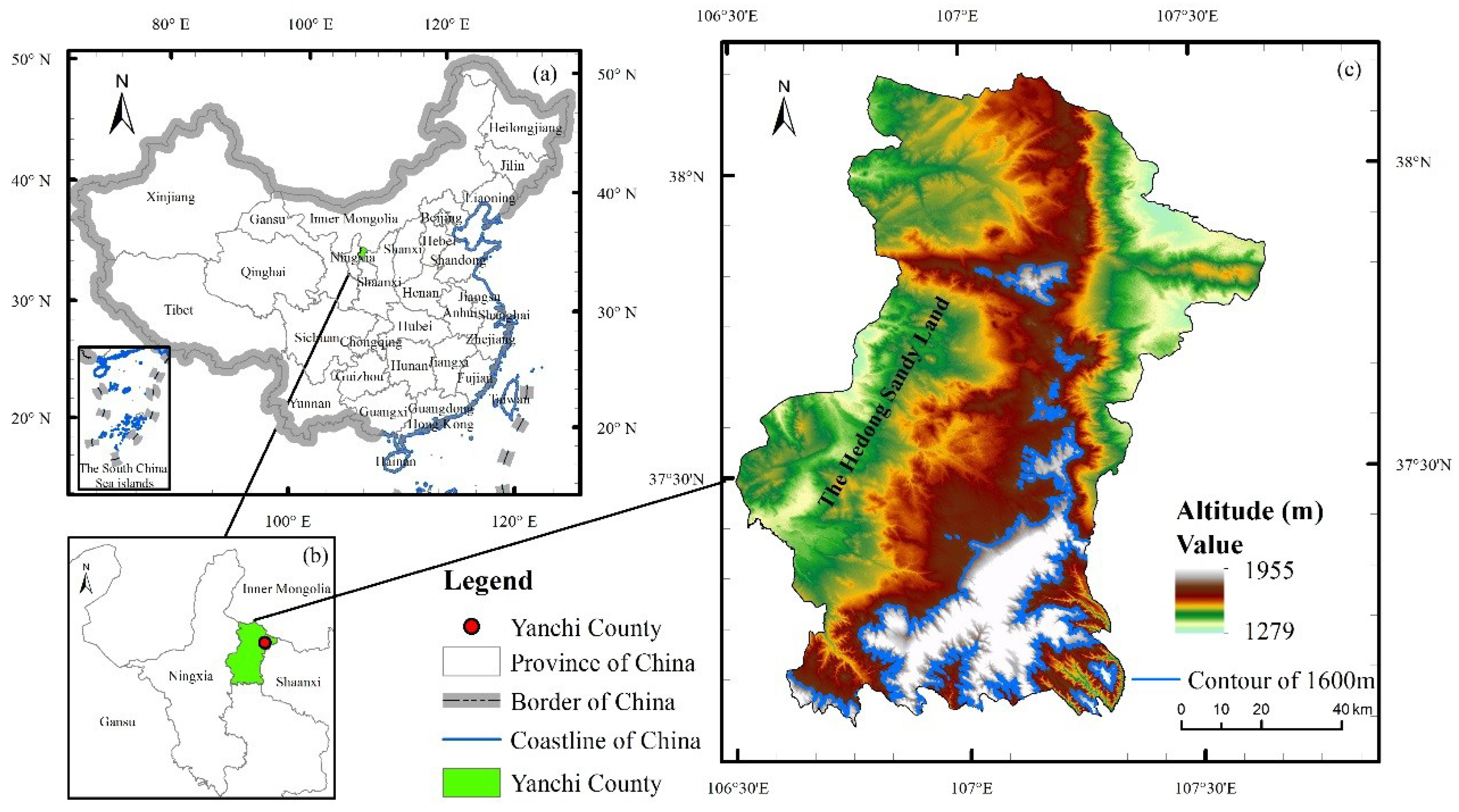
Yanchi County is in the east of Ningxia (37°04’–38°10’ N, 106°30’–107°41’ E) (Figure 1a,b) and covers an area of 6777.97 km2 with an average altitude of 1600 m. The northern part of the 1600-m contour line belongs to the Hedong Sandy Land, with an area of 5729.9 km2, and the south is the loess hilly area of ephedra (Figure 1c). The climate in Yanchi County is a moderate temperate continental climate with an average annual precipitation of 293.1 mm, an average annual evaporation of 2403.7 mm, an average annual wind velocity of 2.7 m/s, and average annual wind and sandstorm days of 24.2 days and 20.6 days, respectively. Water resources in Yanchi County are very scarce and are mainly supplemented by natural precipitation. The vegetation type transfers from dry steppe to desert steppe, including shrubs, grasslands, meadows, sandy vegetation, and desertification grassland vegetation. The soil type is mainly sierozem, followed by dark loessial soil and eolian sandy soil, in addition to loess, a small amount of saline soil, albic soil, and so on. The resource utilization pattern of Yanchi County is determined by the transition zone from a pastoral area to an agricultural area, and the form of desertification is attributed to a transition zone from wind erosion to water erosion. These geographic transitions define the diversity of the region, which includes a farming pastoral zone, a water–wind crisscross erosion region, and an arid and semiarid transition region, which results in the vulnerability of the ecological environment and makes the region become the main area of desertification in China.
2.2. Methodology and Data
2.2.1. The Analytical Framework for the Sustainability of Wind Prevention and Sand Fixation Service
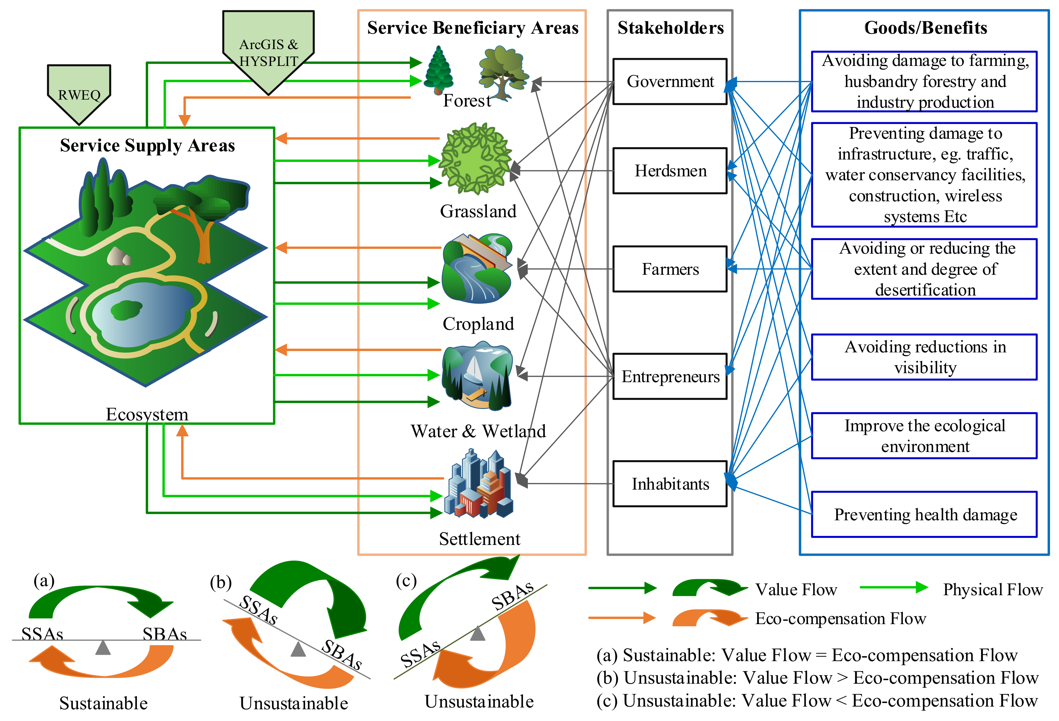
From the perspective of ESF, the WPSF service flows from the SSAs to SBAs to satisfy the demand of the beneficiaries. The goods and benefits include avoiding damage to the regional economy and infrastructure, reducing the extent and degree of desertification, improving the air visibility and ecological environment quality, and preventing health damage. These benefits derive from the physical and value flow of the WPSF service in the SSAs by sacrificing their development opportunities and ecological protection investments. In fact, the physical flow process of the WPSF service implies the process of value transfer, as the amount and location of the physical flow determines the quantity and circulation of the value flow. Therefore, based on the existing physical flow of the WPSF service and combined with the ecosystem service value calculation, we can obtain the value flow for the WPSF service, the amount and direction of which are both the same as the physical flow (Figure 2). The value flow reflects the opportunity cost for the supply of WPSF service and the outflow of ESs from SSAs, which can provide a direct scientific basis for the formulation of an ecological compensation policy [47]. Theoretically speaking, eco-compensation value flow should be borne by the beneficiaries in SBAs to balance the value flow loss and guarantee the sustainability of WPSF service in SSAs. However, there are many stakeholders in the process of value flow and eco-compensation flow. The stakeholders in both SSAs and SBAs tend to seek more development opportunities for their own benefits without considering the ecological environment destruction. Consequently, the eco-compensation flow amount is often less than the value flow. When the eco-compensation flow amount is equal to the value flow, the loss of the SSAs can be compensated to maintain sustainable development (Figure 2a). Otherwise, development in both SSAs and SBAs is unsustainable if the eco-compensation flow amount is unequal to the value flow (Figure 2b,c). The data processing procedures involved in the framework include the following aspects: (1) evaluating the physical amount of WPSF service based on RWEQ model and the areas with positive wind erosion prevented amount can be seen as the SSAs; (2) evaluating the value amount of WPSF service according to the physical amount and ecosystem service value calculation; (3) identifying the flow trajectories of WPSF service by using the HYSPLIT model; (4) distinguishing the SBAs of WPSF service based on the flow trajectories in ArcGIS; (5) visualizing the physical and value flow process based on the physical and value amount of WPSF service and the distribution frequency of the flow trajectories in ArcGIS; and (6) determining the relationship between the value flow and eco-compensation flow of WPSF service to evaluate its sustainability.
2.2.2. Evaluation of the Physical Amount of Wind Prevention and Sand Fixation Service
The reduction in wind erosion caused by vegetation can be seen as the physical amount of WPSF service and represents the difference between the potential wind erosion amount under bare soil conditions and the actual wind erosion amount under vegetation conditions, which can be calculated based on RWEQ model [29,31]. The actual wind erosion is the soil erosion amount under the condition of vegetation coverage in a real scenario, and the potential wind erosion is the soil erosion under bare land conditions without vegetation. When the wind passes through the soil surface, it is blocked by the vegetation, which weakens the wind and reduces the wind erosion. All the calculation formulas are as follows:
where SLr represents the potential wind erosion amount (kg/m2); Qrmax represents the maximum potential sediment transport capacity (kg/m); Sr represents the potential critical plot length (m); SL represents the actual wind erosion amount (kg/m2); Qmax represents the maximum sediment transport capacity (kg/m); S represents the critical plot length (m); G represents the prevented amount of wind erosion (kg/m2), namely, the physical amount of wind prevention and sand fixation service; z represents the calculated downwind distance (m); and WF, EF, SCF, K′, and C correspond to the factor of weather (kg/m), soil erodibility fraction (%), soil crust factor (dimensionless), soil roughness factor (dimensionless), and vegetation (dimensionless), respectively, which can be expressed as follows:
where Wf is the wind factor (m/s3); g represents the gravitational acceleration (m/s2); ρ represents the air density (kg/m3); SW is the soil moisture factor (dimensionless); and SD represents the snow cover factor (dimensionless), which is the ratio of days with no snow cover to the total number of days studied. A snow cover depth less than 25.4 mm indicates no snow cover. u1 represents the threshold wind velocity at a height of 2 m (m/s). The threshold wind velocity for sand lands and sandy grasslands in Yanchi County are 4.88 m/s and 5.17 m/s, respectively, based on observations of wind–sand activities [46]. Because the existing vegetation type is mainly sandy grassland in Yanchi County, the threshold wind velocity for sandy grassland is used to calculate the actual wind erosion amount. u2 represents the monthly average wind velocity at a height of 2 m (m/s). Nd represents the number of days with a monthly average wind velocity that exceeds the threshold wind velocity.
To calculate the WF, daily meteorological data of 24 weather stations (Yanchi, Yinchuan, Taole, Huinong, Wuzhong, Zhongwei, Zhongning, Tongxin, Guyuan, Liupan Moutain, Haiyuan, Xiji, Etuoke Banner, Jingtai, Jingyuan, Huajialing, Jartai, Linhe, Alxa Left Banner, Dingbian, Wu Banner, Huan County, Pingliang, and Tianshui) around Ningxia in 2010 and 2015 were achieved from the National Meteorological Information Center. The meteorological elements of the above stations included daily average wind velocity, maximum wind velocity, average air temperature, highest air temperature, lowest air temperature, average relative humidity, and sunshine duration. The snow cover data, Chinese snow depth long time-series dataset (1979–2016), was derived from the scientific data center of Cold and Arid Regions (http://westdc.westgis.ac.cn). This dataset provides the daily snow thickness distribution data in China from 1 January 1979 to 31 December 2016, with a spatial resolution of 0.25°.
where sa, si, cl, OM, and CaCO3 represent the content of sand, silt, clay, organic matter, and calcium carbonate (%), respectively.
In this study, EF and SCF were assumed to be unchanged over time and were calculated by the soil raster data that was converted from a 1:1,000,000-scale soil data shapefile provided by the Harmonized World Soil Database (HWSD) built by FAO International Institute for Applied System Analysis (IIASA). During the calculation, we converted the classification criteria of soil texture from international in the database to American criteria to meet the factor calculation requirements by using the logistic growth model proposed by Skaggs et al. [48]:
where SC represents the vegetation coverage (%), NDVIveg represents the normalized difference vegetation index (NDVI) value of a highly vegetated grid, and NDVIsoil represents the NDVI value of a bare land grid. NDVIveg and NDVIsoil correspond to the NDVI value at a 95% and 5% cumulative frequency, respectively. NDVI values (spatial resolution 500 m) were derived from the international scientific data mirror website of the computer network information center, Chinese Academy of Sciences (http://www.gscloud.cn):
where α represents the slope gradient and is calculated by a digital elevation model (DEM) in ArcGIS [49]. The DEM data (spatial resolution 30 m) were derived from the Resource and Environment Data Cloud Platform, Chinese Academy of Sciences (CAS) (http://www.resdc.cn).
The function of the WPSF service can indicate the actual sand-fixation capacity of vegetation. However, the function of the WPSF service itself cannot effectively highlight the contribution of the ecosystem to sand fixation due to the influence of climatic factors, such as wind field intensity. To eliminate the impact of climate and emphasize the sand-fixation function of the ecosystem, the ratio of the amount of wind erosion prevented and the potential wind erosion amount under bare soil surface conditions can be defined as the retention rate of the WPSF service:
where F represents the retention rate of the WPSF service (%), G represents the amount of prevented wind erosion (kg/m2), and SLr represents the potential wind erosion amount (kg/m2).
2.2.3. Evaluation of the Value Amount of Wind Prevention and Sand Fixation Service
The economic value of the WPSF service can be reflected in the reduction in surface soil erosion, sediment deposition, and soil fertility protection, which can be calculated from the following formulas:
where VSE is the value of soil erosion reduction (CNY/a) (CNY is the Chinese Currency, as of 18 July 2018, 6.702 CNY = US $1). Soil erosion causes the loss of topsoil and eventually leads to abandoned land. Besides, the land cover type is dominated by grassland in Yanchi County. Therefore, VSE can be estimated based on the opportunity cost of animal husbandry. G represents the prevented wind erosion amount (kg/m2), P0 represents annual benefit per unit area (CNY/m2) of animal husbandry in Yanchi County, and d is soil bulk density (t/m3). In this study, we used the mean soil bulk density of China’s terrestrial ecosystem, which was 1.35 t/m3 [50]. h is the thickness of soil, which is calculated as 1 m [51]. VSD is the value of sediment deposition prevention (CNY/a). According to the law of sediment movement in China’s major river basins, 24% of the sediment lost in soil is deposited in rivers and lakes. VSD can be calculated based on the water storage costs. In the formula, C is the engineering cost of the reservoir (CNY/m3), 6.9 CNY/m3 [52]. VSF is the value of protecting soil fertility (CNY/a), which can be calculated by the price of fertilizer, soil retention, and soil nutrient content. Ci is the average content of nutrients (mainly nitrogen, phosphorus, and potassium) in the soil. According to the soil data, the mean content of nitrogen, phosphorus, and potassium in Yanchi soil was determined to be 0.283%, 0.147%, and 2.07%, respectively. ni is the amount of nitrogen, phosphorus, and potassium maintained in soil, which should be converted into urea, calcium superphosphate, and potassium chloride conversion coefficients, which are 2.164, 4.065, and 1.923, respectively [53]. Pi is the market price of fertilizer (CNY/t). In this study, the national average retail prices of urea, calcium superphosphate, and potassium chloride were taken as the reference basis for the value of Pi, which was 1640 CNY/t, 890 CNY/t, and 2815 CNY/t, respectively.
2.2.4. HYSPLIT Forward Trajectory Simulation
The HYSPLIT model used the advection and diffusion calculations as the trajectories or air parcels moving from their initial location based on the Lagrangian approach [54]. The trajectory of a particle can be seen as the integration of the particle position vector in space and time under the hypothesis that the particle moves passively following the wind. In this research, HYSPLIT was used to simulate the forward trajectory of the WPSF service. The initial position of the simulated 5-day forward trajectories was centered at 37.8° N, 107.38° E (i.e., Yanchi), with a starting elevation at 500 m above ground level. The trajectories were only simulated for every 6 h from 12:00 a.m. on 1 January to 12:00 a.m. on 31 December in 2010 and 2015, when the maximum 10-min average wind velocity in 1 h by 6-hourly wind speed records for one day at Yanchi meteorological station was no less than the threshold wind velocity. Besides, during the simulation, the NCEP/National Center for Atmospheric Research (NCAR) reanalysis data were needed.
2.2.5. The SBAs of the Wind Prevention and Sand Fixation Service
The areas that the dust trajectories pass through are the SBAs of the WPSF service. The identification of SBAs of Yanchi County’s WPSF service was based on the maximum boundary of dust transmission originating from Yanchi County, namely, the areas that the dust trajectories pass through under bare soil without vegetation. The benefits people receive from the WPSF service include avoiding sand deposition and air pollution to agriculture, husbandry, forestry, industry, infrastructure (e.g., traffic, water conservancy facilities, construction, communication networks, etc.), ecological environment (e.g., visibility, air quality, etc.), and human health. The more dense the transmission trajectories of WPSF service in the SBAs, the greater the benefits to humans. The SBAs were distinguished by the interpolation of the flow trajectories of the WPSF service with HYSPLIT [8,55]. The spatial resolution of the interpolated grid was 1° × 1° and the value of each grid was the frequency with which the trajectories passed through, which was calculated as
where pi is the frequency of the trajectories passed through pixel i; Li is the number of trajectories that passed through pixel i; and L is the total number of simulated trajectories. A higher pi implies that the people in those pixels benefit more from the WPSF service flow than the people in other grid cells.
3. Results
3.1. Spatial Distribution of the Wind Prevention and Sand Fixation Service in Yanchi County
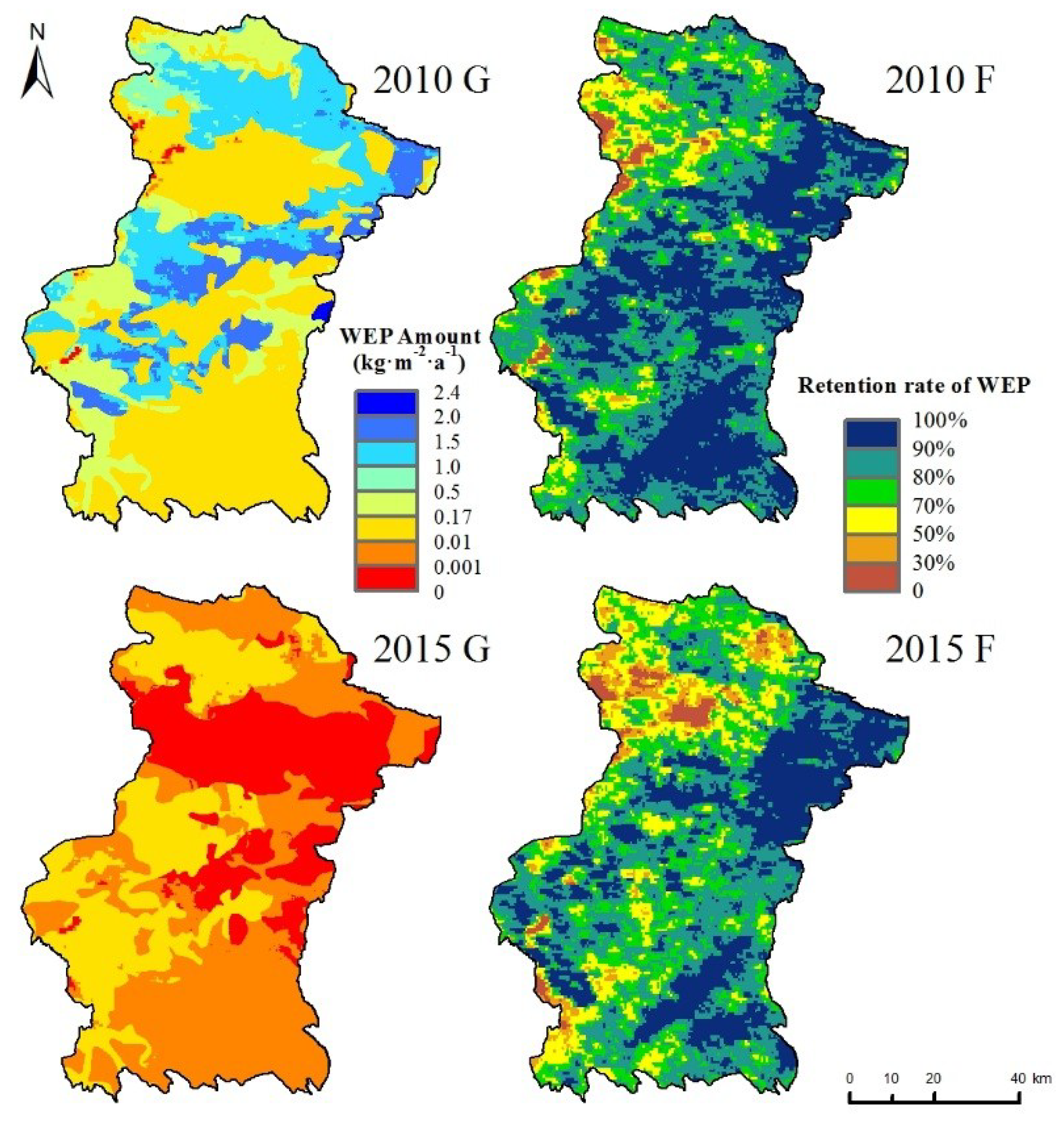
The total amount of wind erosion prevented for the whole ecosystem in Yanchi County was 3.71 × 10⁹ kg in 2010 and 0.08 × 10⁹ kg in 2015, with an average amount of prevented wind erosion per unit area of 0.55 kg·m−2·a−1 and 0.01 kg·m−2·a−1, respectively, and a maximum average amount of 2.41 kg·m−2·a−1 and 0.17 kg·m−2·a−1, respectively. Compared with 2010, the amount of prevented wind erosion decreased by 97.9% in 2015. The spatial distribution pattern of the prevented wind erosion in Yanchi County was basically the same in 2010 and 2015 (Figure 3), with high-value areas in northern and midwestern Yanchi (i.e., the Hedong Sandy Land) and low-value areas in the loess hilly area of ephedra in the southeast. The average retention of the WPSF service in Yanchi County was 83.40% in 2010 and 78.11% in 2015. In contrast to the spatial distribution pattern of prevented wind erosion, areas with high retention rates were mainly located in areas with high vegetation coverage in the east, while low retention rate areas were located in the Hedong Sandy Land region to the east. Conserving the grasslands is the most effective way to curb soil wind erosion, as the grasslands can weaken climate-driven forces, protect surface soil from wind abrasion, change the soil composition, and promote the formation of soil aggregates to reduce soil wind erosion. The area with the highest retention rate of prevented wind erosion was also the area with the best grassland coverage.
3.2. Flow Trajectories of the Wind Prevention and Sand Fixation Service
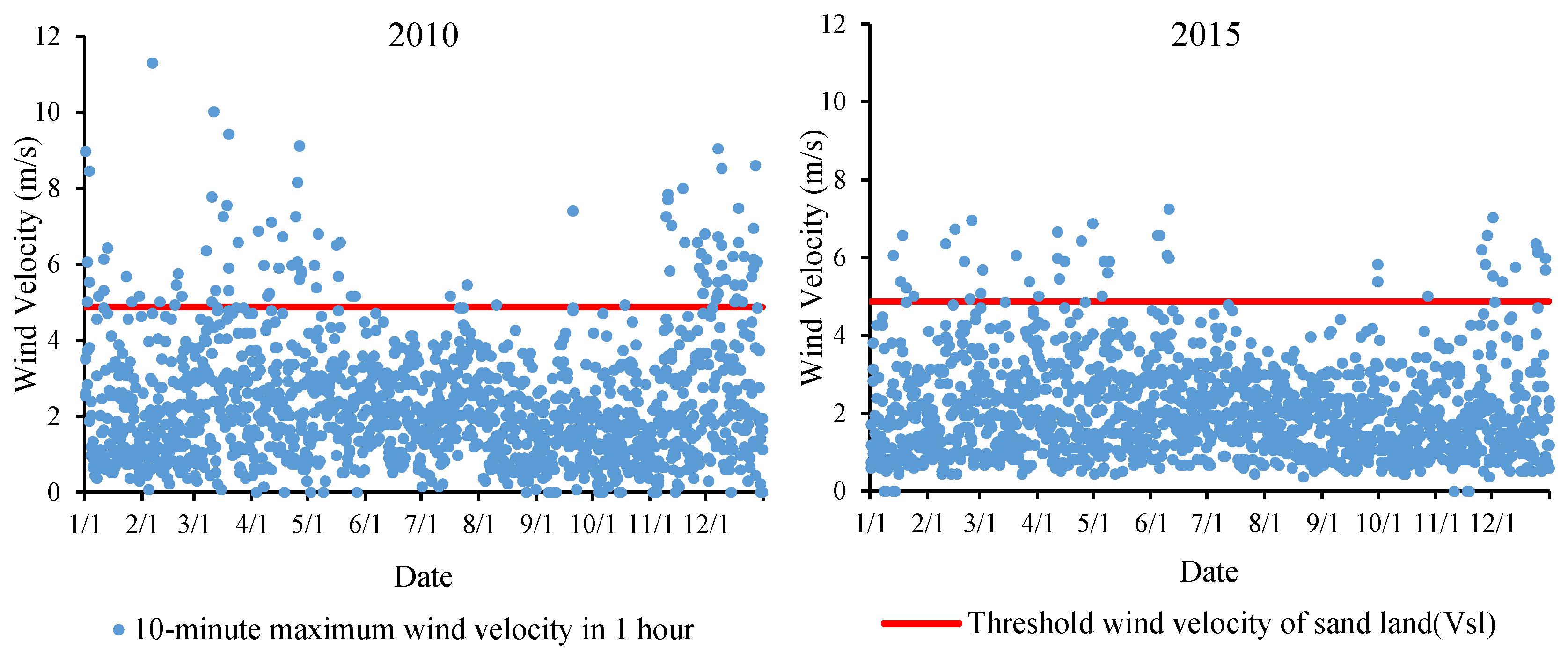
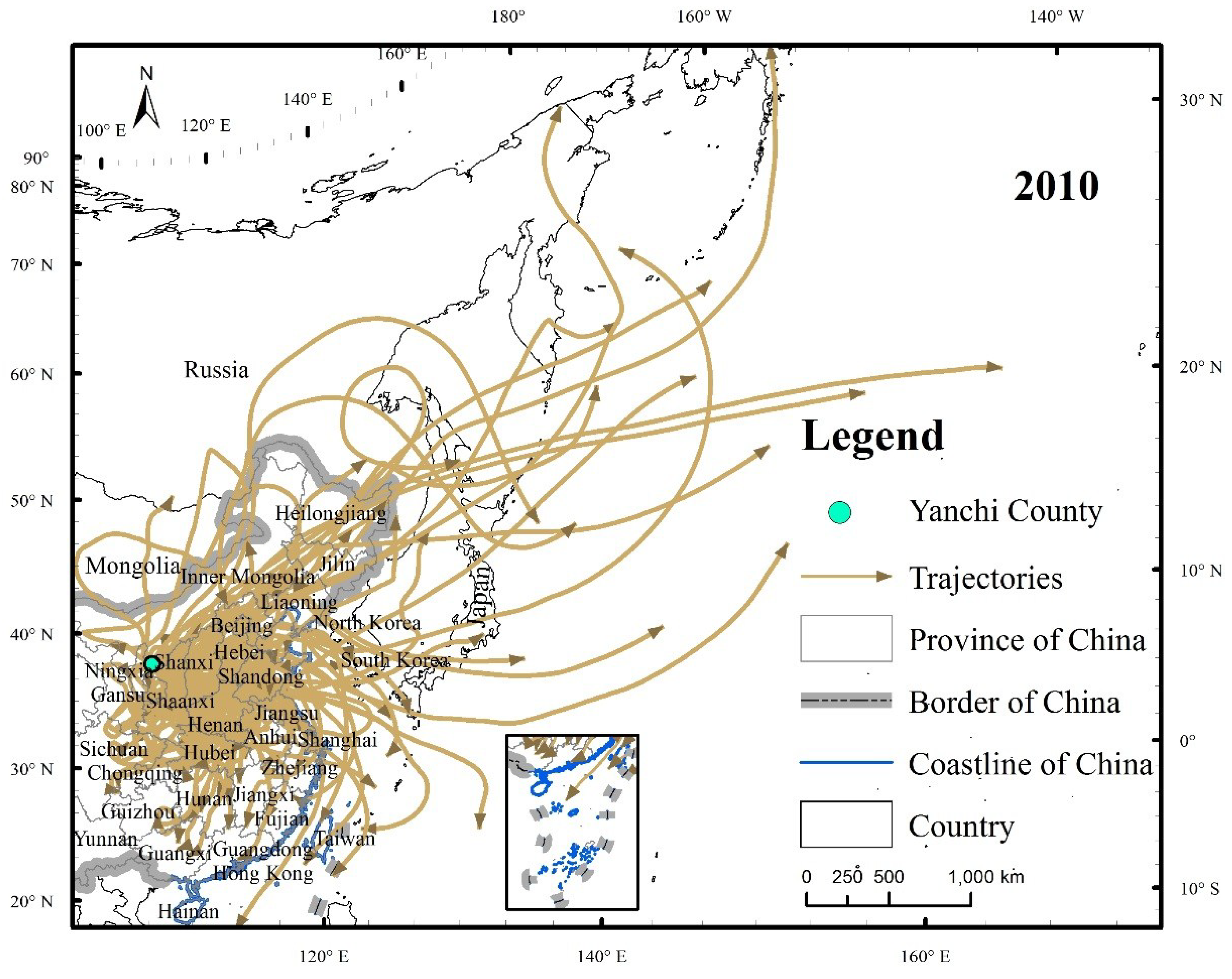
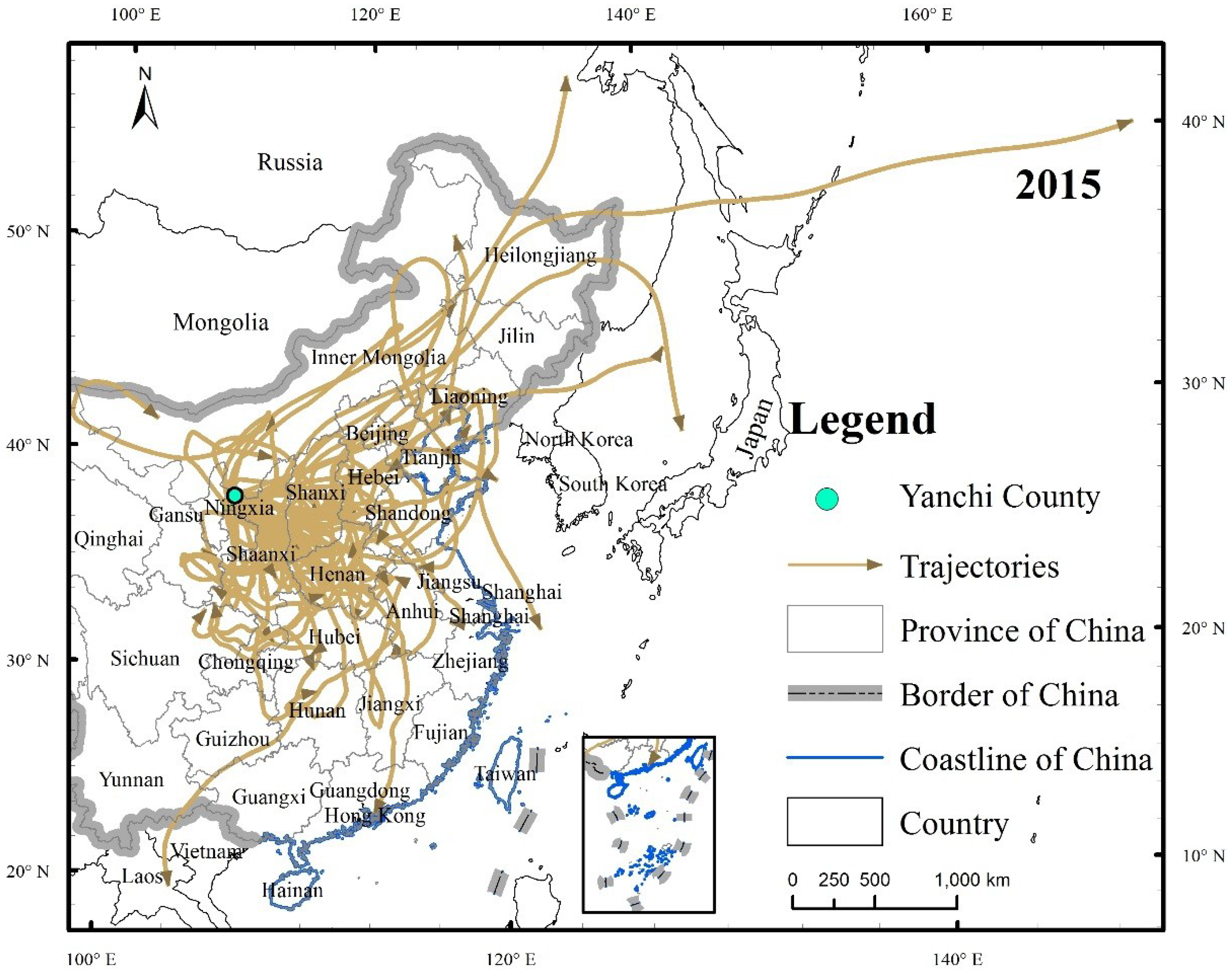
There were 1460 6-h wind velocity records in both 2010 and 2015 (Figure 4). The maximum wind velocity at a height of 2 m was 11.3 m/s in 2010 and 7.3 m/s in 2015, the minimum wind velocity was 0 m/s during both years, and the means were 2.3 m/s and 2.8 m/s, respectively. In 2010 and 2015, 99 and 45 wind velocity records exceeded the threshold wind velocity for the sand land (≥5.17 m/s), which corresponded to trajectories of 99 and 45, respectively (Figure 5). The simulated flow trajectories of WPSF service in Yanchi County mainly passed over East Asia, including north-central and eastern China, the Korean Peninsula, Japan, Mongolia, and eastern Russia in 2010 and 2015 and extended over Laos and Vietnam in 2015. Thus, the benefits of the WPSF service extended to countries other than China. The density of the dust transmission paths increased with the increase in transmission distance. The areas over which the trajectories flowed within China were mainly the Shaanxi, Shanxi, Hebei, Shandong, Beijing, Tianjin, Henan, Hubei, Jiangsu, and Liaoning Provinces, which were consistent with the results of Li et al. [56]. In general, the density of the trajectories decreased with an increase in the transmission distance, indicating that prevented wind erosion and sand fixation exhibit spatial proximity characteristics.
3.3. Areas Benefitting from the Wind Prevention and Sand Fixation Service
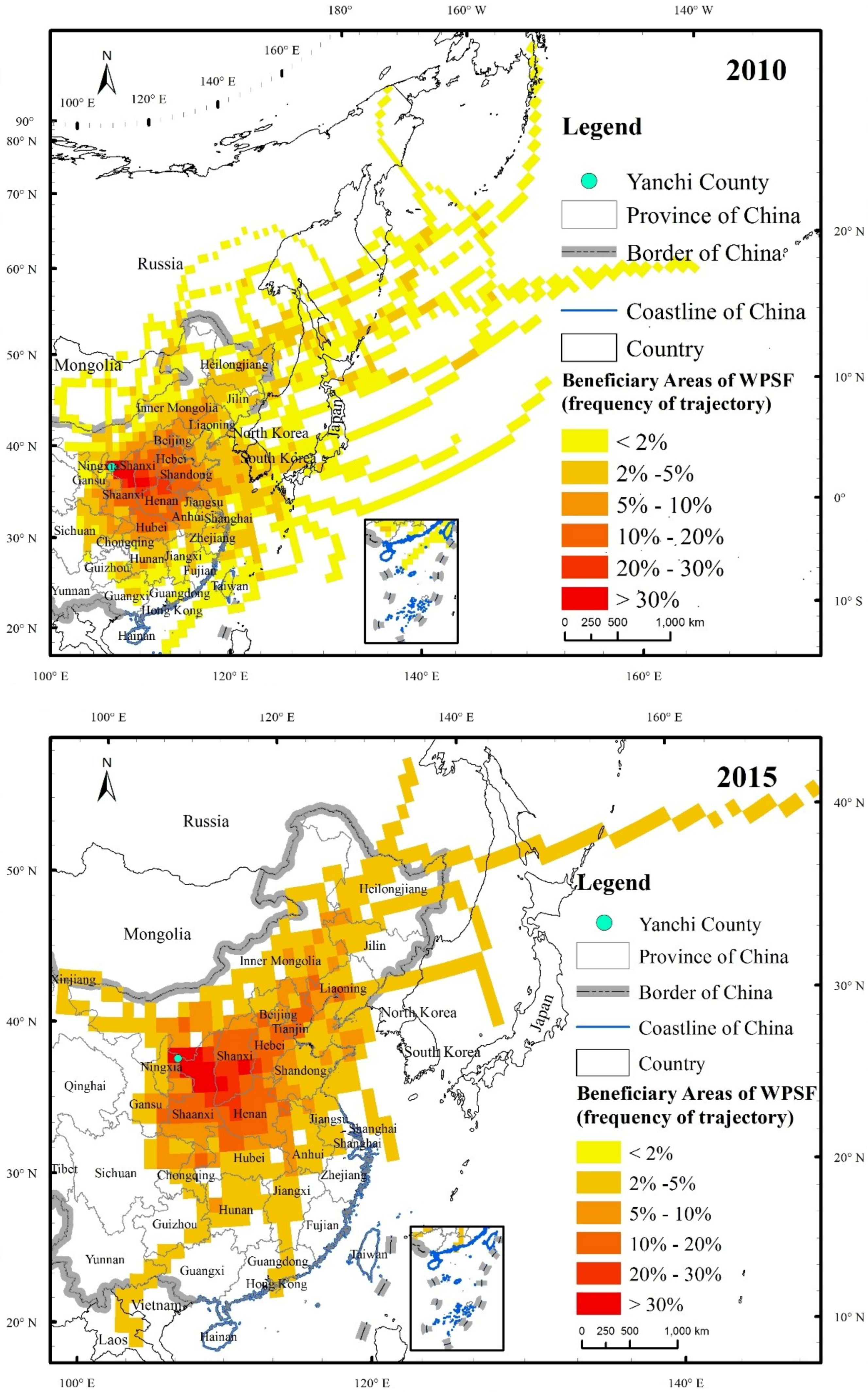
The spatial distribution of the areas benefitting from the WPSF service can be derived from the spatial interpolation of flow paths of the WPSF service (i.e., the areas of the dust transmission path that passed overhead can be regarded as the SBAs of the WPSF service). The ecosystem area that benefitted from the WPSF service in Yanchi County was estimated to be 1153.2 × 104 km2 in 2010 and 397.2 × 10⁴ km2 in 2015. In China, the SBAs were mostly in the eastern and north-central regions of the country (Figure 6), and they were estimated to be 392.4 × 10⁴ km2 in 2010 and 298.4 × 10⁴ km2 in 2015, which represented 40.9% and 31.1% of the total area of China, respectively, and indicated that the area of WPSF SBAs in Yanchi County was significantly reduced in 2015, especially for offshore areas. The grids with more than 10% of the trajectories were concentrated in the Shaanxi, Shanxi, Henan, western Shandong, Hebei, Beijing, and northern Hubei Provinces, and the frequencies of those in the Yan’an district, north-central Shaanxi and Linfen, and southwest Shanxi Province were greater than 30%. People in these higher frequency grids benefitted more from the WPSF service flow due to the ecosystems in Yanchi County than other grids. Overall, the area of the high-frequency region in 2015 decreased relative to that in 2010.
3.4. The Physical Flow of the Wind Prevention and Sand Fixation Service
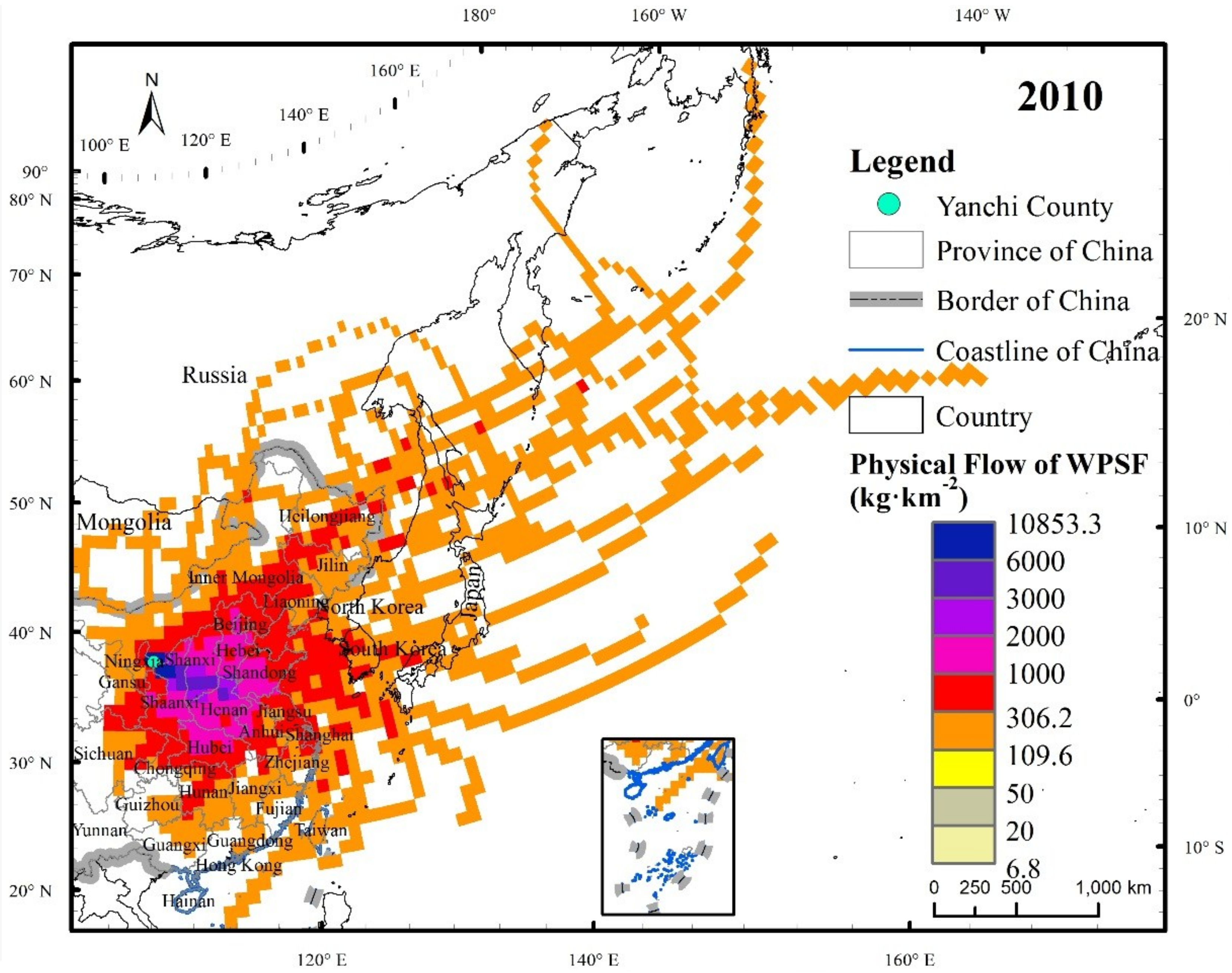
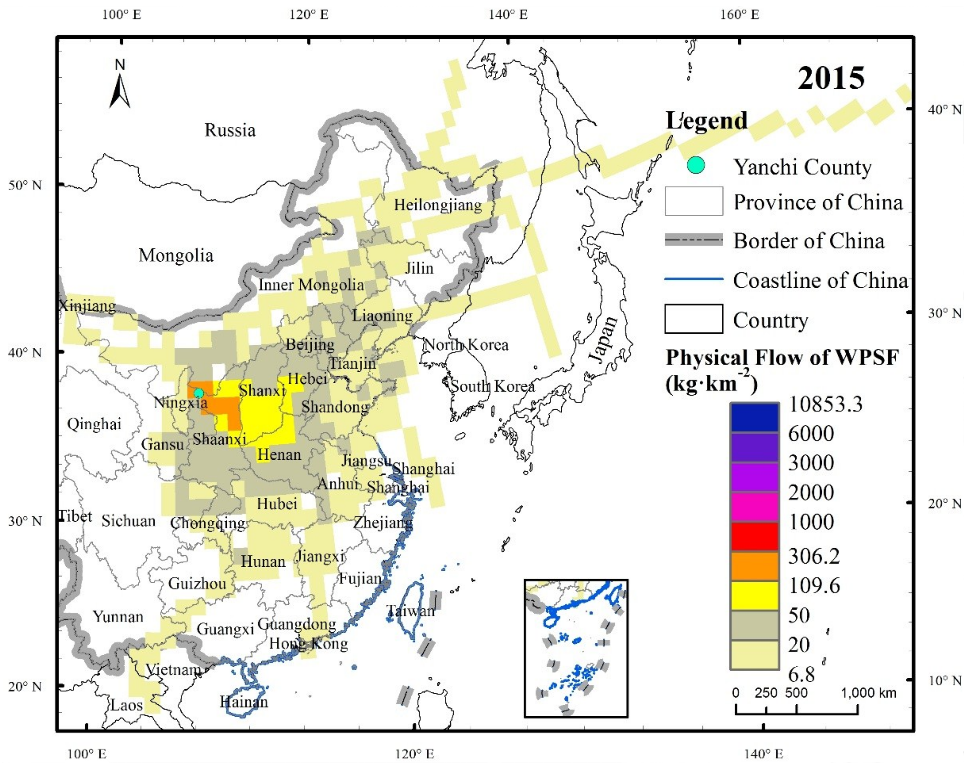
The dust flow path established a spatiotemporal relationship between the SSAs (the ecosystem of Yanchi County) and SBAs. Sediment deposition during dust transmission was closely related to the distribution frequency of the trajectories. The higher the trajectory frequency, the more dust deposition and the higher the effect of the WPSF service. The amount of dust transmission during the flow of the WPSF service can be defined as the physical flow of the WPSF service. In 2010 and 2015, the physical flow amount of the WPSF service in the SBAs was equal to the total prevented wind erosion amounts in 2010 and 2015. Among them, the physical flow amounts of the WPSF service obtained by the SBAs in China were 2.64 × 10⁹ and 0.07 × 10⁹ kg, which accounted for 71.11% and 91.32% of the total annual physical flow amount, and the average physical flow density was 597.16 kg·km−2 and 20.23 kg·km−2, respectively. The spatial distribution of the physical flow of the WPSF service in the SBAs can be derived from the distribution frequency of the dust transmission trajectory (Figure 7), with a high-value center in Shaanxi, Shanxi, and Hunan to the southeast. The physical flow amount of Shaanxi was the largest, which was 0.44 × 10⁹ kg in 2010 and 0.01 × 10⁹ kg in 2015, and the average physical flow density was 2150.35 kg·km−2 and 69.65 kg·km−2, respectively. In general, an improvement in the ecological environment that can reduce the wind erosion directly in Yanchi County has an obvious impact on sand and dust deposition in SBAs with a high physical flow amount, while this same improvement has little or no impact in Yunnan, Fujian, or Taiwan to the southwest or southeast.
4. Discussion
4.1. Implications for Eco-Compensation Based on Ecosystem Service Value Flow
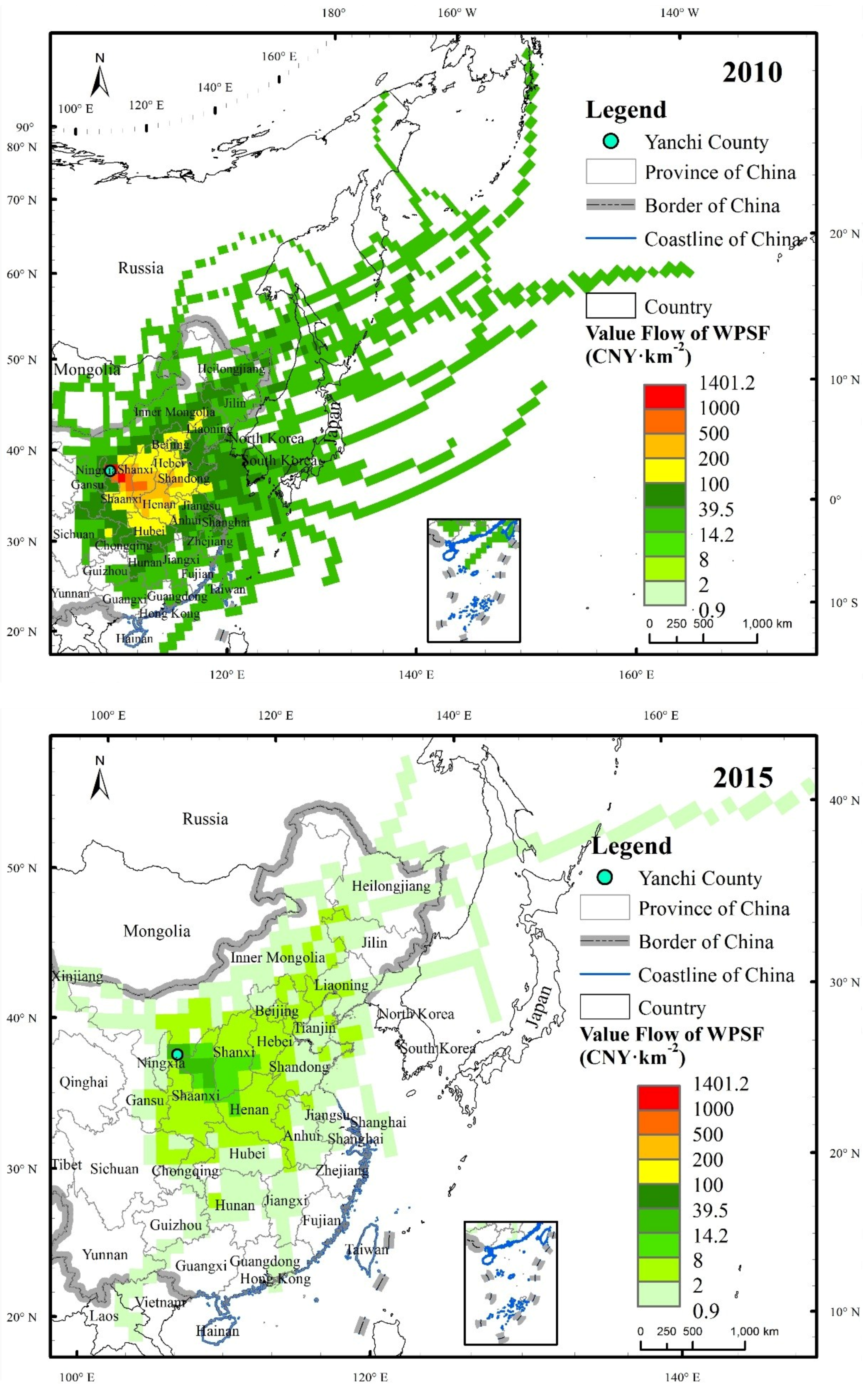
Human activities, such as overgrazing and farming, increase the desertification of grasslands and reduce vegetation coverage, thereby aggravating wind erosion. Though many ecological protection policies have been implemented in Yanchi County, there will be inevitable conflict between the economic interests of farmers/herdsmen and ecological policy if there is no corresponding sufficient economic compensation measures, effective guidance, or industrial structure adjustment [57]. By using an alternative cost method, the values of the WPSF service in Yanchi County in 2010 and 2015 were 479.46 million CNY and 10.22 million CNY, respectively. The value flows in SBAs in China were 340.96 million CNY and 9.33 million CNY, respectively, which accounted for 71.11% and 91.32%, respectively, where the spatial distributions were the same as those of the physical flow (Figure 8). The value flow of Shaanxi Province was the largest (57.16 million CNY in 2010 and 1.85 million CNY in 2015), and the average value flow density was 277.6 CNY·km−2 and 9.0 CNY·km−2, respectively. These value flows can provide a scientific basis for the formulation of the eco-compensation standard and be directly used to encourage the local residents in the SSAs to take measures to prevent further wind erosion (e.g., reducing grazing and returning farmland to forests and grasslands).
4.2. The Mismatches between the Value Flow and Eco-Compensation Flow of the Wind Prevention and Sand Fixation Service
Although the government implemented some ecological engineering measures, the farmers and herdsmen still had difficulties in establishing ecological awareness under the undeveloped economic pressure, which led to widespread illegal grazing [58] and unsustainable WPSF service supply. The fiscal subsidies related to grazing prohibition was very low and mainly funded by the government. Besides, the related policies were difficult to implement in contrast to the cropland protection program. However, the SBAs of the WPSF service for Yanchi County were mainly located in the eastern region, which has a higher economic development level, and the flow of the WPSF service greatly contributed to their economic development. Therefore, the downwind SBAs should contribute some ecological compensation to rectify the lack of existing ecological protection funds. However, there are no corresponding horizontal ecological compensation measures taken by the government or other stakeholders, partly due to the lack of a scientific foundation for policy making, which has led to the apparent mismatch between the value flow and eco-compensation flow of the WPSF service. The unsustainable mismatches can be solved by horizontal eco-compensation based on the physical and value flow analysis of the WPSF service, the improvement of the government’s management, and the involvement of every stakeholder.
4.3. Restrictions and Prospects
This study delineated the physical flow and value flow of the WPSF service from the SSAs in Yanchi County to the downwind SBAs, which can serve as an objective reference for an ecological compensation policy. However, there are still some restrictions in the research. The sand and dust transmission was simulated under these hypotheses: (1) an abundant sand source existed in the study area and (2) sand and dust would transport to the downwind areas as long as the wind velocity was no less than the threshold. The simplification of the flow path simulation of dust transmission based on the path frequency without considering the sequence of different sand grain sediments and other meteorological factors can influence the accuracy of the physical and value flows of the WPSF service to a certain extent. Due to the lack of field observation data, we did not consider the seasonal variation in the wind velocity threshold, which resulted in a lack of analysis on the seasonal difference in the flow of the WPSF service. Besides, we simplified the spatial difference of wind velocity in the SSAs and selected Yanchi meteorological station as a representative site to simulate the flow trajectories. Furthermore, more sophisticated models, including existing wind erosion models and sand deposition simulation models, should be developed to quantify the flow of prevented wind erosion from SSAs to SBAs. In the future, these restrictions above should be considered in the analysis of the WPSF service flow and more attention could be paid to the integration of wind erosion and air quality models.
5. Conclusions
Spatial visualization of the physical and value flows of ESs is beneficial and intuitive to reveal the relationship between SSAs and SBAs. The WPSF service has an obvious spatiotemporal flow attribute which can be traced by the sand and dust movement. This study analysed the spatiotemporal pattern of the WPSF service by the RWEQ model and identified the SBAs based on dust transmission paths simulated by the HYSPLIT model, which confirmed the physical and value flows of the WPSF service based on the distribution frequencies of the dust flow paths. We concluded that (1) the total amount of prevented wind erosion for the whole ecosystem in Yanchi County varied significantly under different land cover and meteorological condition, which was 3.71 × 10⁹ kg in 2010 and 0.08 × 10⁹ kg in 2015, and the retention of WPSF service in Yanchi County was 83.40% in 2010 and 78.11% in 2015. The areas with high retention rates were mainly located in areas to the east with high vegetation coverage. Therefore, conserving vegetation, especially the grasslands in arid and semiarid areas, is necessary for the improvement of the WPSF service and the downwind beneficiary areas. (2) There were 99 and 45 trajectories for the WPSF service in 2010 and 2015, respectively, which mainly passed over East Asia and had spatial proximity characteristics. (3) The areas that benefitted from the WPSF service due to ecosystems in Yanchi County were estimated to be 1153.2 × 104 km2 in 2010 and 397.2 × 10⁴ km2 in 2015. The areas with higher frequencies received more benefits from the WPSF service flow than other areas. (4) The SBAs in China were estimated to be 392.4 × 10⁴ km2 in 2010 and 298.4 × 10⁴ km2 in 2015. Though the areas of SBAs varied significantly, their extent within China mainly concentrated in eastern and north-central China, through which more than 10% of the trajectories passed. The frequencies of trajectories were greatest in the Yan’an district, north-central Shaanxi and Linfen, and southwest Shanxi Province. (5) The spatial distribution of the physical and value flows of the WPSF service was identical in each year. The flow rates of the physical and value flows of the SBAs in China were the same, accounting for 71.11% in 2010 and 91.32% in 2015. There were mismatches between the value flow and eco-compensation flow, which was unsustainable. From the perspective of ESF, we can evaluate the sustainability of WPSF service by connecting the provision and beneficiary areas at the same time, for the realization of ESs value is a comprehensive process that includes not only the supply but also the demand side. This study established an analytical framework for the sustainability of WPSF service by incorporating an existing wind erosion model that can be applied to other areas and has important theoretical significance for the study of ESF and practical significance for the formulation of ecological protection policies and sustainable development.
Author Contributions
Y.X. and J.X. conceived and co-designed the research. J.X. analysed the data and wrote the manuscript. G.X. and Y.J. polished the language and revised the paper. Y.W. and J.X. collected the data.
Funding
This study was supported by the National Key Research and Development Program of China (Grant No. 2016YFC0503403 and 2016YFC0503706), the Demonstration Project for Industrial Integration and Development (Grant No. YES-16-10-1001), the Science and Technology Innovation Pilot Fund Project of Ningxia Academy of Agriculture and Forestry Sciences (Grant No. nkyz-16-1001), soft science research of Ministry of Agriculture and Rural Affairs (Grant No. 2018084) and the Natural Science Foundation of Zhejiang Province, China (Grant No. LY18D010001).
Conflicts of Interest
The authors declare no conflict of interest.
References
- Schröter, M.; Stumpf, K.H.; Loos, J.; van Oudenhoven, A.P.E.; Böhnke-Henrichs, A.; Abson, D.J. Refocusing ecosystem services towards sustainability. Ecosyst. Serv. 2017, 25, 35–43. [Google Scholar] [CrossRef]
- Costanza, R.; Groot, R.D.; Braat, L.; Kubiszewski, I.; Fioramonti, L.; Sutton, P.; Farber, S.; Grasso, M. Twenty years of ecosystem services: How far have we come and how far do we still need to go? Ecosyst. Serv. 2017, 28, 1–16. [Google Scholar] [CrossRef]
- Costanza, R. Ecosystem services: Multiple classification systems are needed. Biol. Conserv. 2008, 141, 350–352. [Google Scholar] [CrossRef]
- Fisher, B.; Turner, R.K.; Morling, P. Defining and classifying ecosystem services for decision making. Ecol. Econ. 2009, 68, 643–653. [Google Scholar] [CrossRef] [Green Version]
- Syrbe, R.U.; Walz, U. Spatial indicators for the assessment of ecosystem services: Providing, benefiting and connecting areas and landscape metrics. Ecol. Indic. 2012, 21, 80–88. [Google Scholar] [CrossRef]
- Burkhard, B.; Kroll, F.; Nedkov, S.; Müllera, F. Mapping ecosystem service supply, demand and budgets. Ecol. Indic. 2012, 21, 17–29. [Google Scholar] [CrossRef]
- Turner, W.R.; Brandon, K.; Brooks, T.M.; Costanza, R.; Fonseca, G.A.B.; Portela, R. Global conservation of biodiversity and ecosystem services. Bioscience 2007, 57, 868–873. [Google Scholar] [CrossRef]
- Bagstad, K.J.; Johnson, G.W.; Voigt, B.; Villa, F. Spatial dynamics of ecosystem service flows: A comprehensive approach to quantifying actual services. Ecosyst. Serv. 2013, 4, 117–125. [Google Scholar] [CrossRef]
- Serna-Chavez, H.M.; Schulp, C.J.E.; Bodegom, P.M.V.; Bouten, W.; Verburg, P.H.; Davidson, M.D. A quantitative framework for assessing spatial flows of ecosystem services. Ecol. Indic. 2014, 39, 24–33. [Google Scholar] [CrossRef]
- Liu, J.G.; Hull, V.; Batistella, M.; De Fries, R.; Dietz, T.; Fu, F.; Hertel, T.W.; Izaurralde, R.C.; Lambin, E.F.; Li, S.X.; et al. Framing sustainability in a telecoupled world. Ecol. Soc. 2013, 18, 26. [Google Scholar] [CrossRef]
- Liu, J.G.; Yang, W. Integrated assessments of payments for ecosystem services programs. Proc. Natl. Acad. Sci. USA 2013, 110, 16297–16298. [Google Scholar] [CrossRef] [PubMed] [Green Version]
- Liu, J.G.; Yang, W.; Li, S. Framing ecosystem services in the telecoupled Anthropocene. Front. Ecol. Environ. 2016, 14, 27–36. [Google Scholar] [CrossRef]
- Schröter, M.; Remme, R.P.; Hein, L. How and where to map supply and demand of ecosystem services for policy-relevant outcomes? Ecol. Indic. 2012, 23, 220–221. [Google Scholar] [CrossRef]
- Jiang, C.; Li, D.Q.; Wang, D.W.; Zhang, L.B. Quantification and assessment of changes in ecosystem service in the Three-River Headwaters Region, China as a result of climate variability and land cover change. Ecol. Indic. 2016, 66, 199–211. [Google Scholar] [CrossRef]
- Goldenberg, R.; Kalantari, Z.; Cvetkovic, V.; Mörtberg, U.; Deal, B.; Destouni, G. Distinction, quantification and mapping of potential and realized supply-demand of flow-dependent ecosystem services. Sci. Total Environ. 2017, 593–594, 599–609. [Google Scholar] [CrossRef] [PubMed]
- Li, D.L.; Wu, S.Y.; Liu, L.B.; Liang, Z.; Li, S.C. Evaluating regional water security through a freshwater ecosystem service flow model: A case study in Beijing-Tianjin-Hebei region, China. Ecol. Indic. 2017, 81, 159–170. [Google Scholar] [CrossRef]
- Liu, J.G.; Hull, V.; Luo, J.Y.; Yang, W.; Liu, W.; Viña, A.; Vogt, C.; Xu, Z.C.; Yang, H.B.; Zhang, J.D.; et al. Multiple telecouplings and their complex interrelationships. Ecol. Soc. 2015, 20, 44. [Google Scholar] [CrossRef]
- Tonini, F.; Liu, J.G. Telecoupling Toolbox: Spatially explicit tools for studying telecoupled human and natural systems. Ecol. Soc. 2017, 22, 11. [Google Scholar] [CrossRef]
- Fang, B.L.; Tan, Y.; Li, C.B.; Cao, Y.J.; Liu, J.G.; Schweizer, P.J.; Shi, H.Q.; Zhou, B.; Chen, H.; Hu, Z.L. Energy sustainability under the framework of telecoupling. Energy 2016, 106, 253–259. [Google Scholar] [CrossRef]
- Liu, J.G. Forest sustainability in China and implications for a telecoupled world. Asia Pac. Policy Stud. 2014, 1, 230–250. [Google Scholar] [CrossRef]
- Liu, J.G.; Hull, V.; Moran, E.; Nagendra, H.; Swaffield, S.R.; Turner, B.L. Applications of the Telecoupling Framework to Land-Change Science. In Rethinking Global Land Use in an Urban Era; MIT Press: Cambridge, MA, USA, 2014; pp. 119–139. [Google Scholar]
- Hulina, J.; Bocetti, C.; Campa, H.; Hull, V.; Yang, W.; Liu, J.G. Telecoupling framework for research on migratory species in the Anthropocene. Elem. Sci. Anthr. 2017, 5, 5. [Google Scholar] [CrossRef]
- Deines, J.M.; Liu, X.; Liu, J.G. Telecoupling in urban water systems: An examination of Beijing’s imported water supply. Water Int. 2016, 41, 251–270. [Google Scholar] [CrossRef]
- Roels, B.; Donders, S.; Werger, M.J.A.; Dong, M. Relation of wind-induced sand displacement to plant biomass and plant sand-binding capacity. Acta Bot. Sin. 2001, 43, 979–982. [Google Scholar]
- Bagnold, R.A. The Physics of Blown Sand and Desert Dune; Chapman and Hall: London, UK, 1941; pp. 182–256. [Google Scholar]
- Burgess, R.C.; McTainsh, G.H.; Pitblado, J.R. An index of wind erosion in Australia. Aust. Geogr. Stud. 1989, 27, 98–110. [Google Scholar] [CrossRef]
- McTainsh, G.H.; Lynch, A.W.; Burgess, R.C. Wind erosion in eastern Australia. Aust. J. Soil Res. 1990, 28, 323–339. [Google Scholar] [CrossRef]
- McTainsh, G.H.; Lynch, A.W.; Tews, E.K. Climatic control upon dust storm occurrence in eastern Australia. J. Arid Environ. 1998, 39, 457–466. [Google Scholar] [CrossRef]
- Fryrear, D.W.; Saleh, A.; Bilbro, J.D.; Schromberg, H.M.; Stout, J.E.; Zobeck, T.M. Revised Wind Erosion Equation. Tech. Bull. 1998, 1, 33–54. [Google Scholar]
- Du, H.; Xue, X.; Wang, T.; Deng, X.H. Assessment of wind-erosion risk in the watershed of the Ningxia-Inner Mongolia Reach of the Yellow River, northern China. Aeolian Res. 2015, 17, 193–204. [Google Scholar] [CrossRef]
- Du, H.Q.; Dou, S.T.; Deng, X.H.; Xue, X.; Wang, T. Assessment of wind and water erosion risk in the watershed of the Ningxia-Inner Mongolia Reach of the Yellow River, China. Ecol. Indic. 2016, 67, 117–131. [Google Scholar] [CrossRef]
- Jiang, L.; Xiao, Y.X.; Rao, E.M.; Wang, L.Y.; Ouyang, Z.Y. Effects of land use and cover change (LUCC) on ecosystem sand fixing service in Inner Mongolia. Acta Ecol. Sin. 2016, 36, 3734–3747. (In Chinese) [Google Scholar]
- Grell, G.A.; Peckham, S.E.; Schmitz, R.; McKeen, S.A.; Frost, G.; Skamarock, W.C.; Eder, B. Fully coupled “online” chemistry within the WRF model. Atmos. Environ. 2005, 39, 6957–6975. [Google Scholar] [CrossRef]
- Gong, S.L.; Lavoué, D.; Zhao, T.L.; Huang, P.; Kaminski, J.W. GEM-AQ/EC, an on-line global multi-scale chemical weather modelling system: Model development and evaluation of global aerosol climatology. Atmos. Chem. Phys. 2012, 12, 8237–8256. [Google Scholar] [CrossRef] [Green Version]
- Dennis, R.L.; Byun, D.W.; Novak, J.H.; Galluppi, K.J.; Carlie, J.C.; Vouk, M.A. The next generation of integrated air quality modeling: EPA’s models-3. Atmos. Environ. 1996, 30, 1925–1938. [Google Scholar] [CrossRef]
- Stein, A.F.; Draxler, R.R.; Rolph, G.D.; Stunder, B.J.B.; Cohen, M.D.; Ngan, F. NOAA’s HYSPLIT Atmospheric Transport and Dispersion Modeling System. Bull. Am. Meteorol. Soc. 2015, 96, 2059–2077. [Google Scholar] [CrossRef]
- Engling, G.; He, J.; Betha, R.; Balasubramanian, R. Assessing the regional impact of Indonesian biomass burning emissions based on organic molecular tracers and chemical mass balance modeling. Atmos. Chem. Phys. 2014, 14, 8043–8054. [Google Scholar] [CrossRef] [Green Version]
- Li, W.; Wang, C.; Wang, H.Q.J.; Chen, J.W.; Yuan, C.Y.; Li, T.C.; Wang, W.T.; Shen, H.Z.; Huang, Y.; Wang, R.; et al. Distribution of atmospheric particulate matter (PM) in rural field, rural village and urban areas of northern China. Environ. Pollut. 2014, 185, 134–140. [Google Scholar] [CrossRef] [PubMed] [Green Version]
- Lv, B.L.; Zhang, B.; Bai, Y.Q. A systematic analysis of PM2.5 in Beijing and its sources from 2000 to 2012. Atmos. Environ. 2015, 124, 98–108. [Google Scholar] [CrossRef]
- Escudero, M.; Stein, A.; Draxler, R.R.; Querol, X.; Alastuey, A.; Castillo, S.; Avila, A. Determination of the contribution of northern Africa dust source areas to PM10 concentrations over the central Iberian Peninsula using the Hybrid Single-Particle Lagrangian Integrated Trajectory model (HYSPLIT) model. J. Geophys. Res. 2006, 111, D06210. [Google Scholar] [CrossRef]
- Draxler, R.R.; Gillette, D.A.; Kirkpatrick, J.S.; Heller, J. Estimating PM air concentrations from dust storms in Iraq, Kuwait and Saudi Arabia. Atmos. Environ. 2001, 35, 4315–4330. [Google Scholar] [CrossRef]
- Draxler, R.R. Meteorological factors of ozone predictability at Houston, Texas. J. Air Waste Manag. Assoc. 2000, 50, 259–271. [Google Scholar] [CrossRef] [PubMed]
- Stein, A.F.; Isakov, V.; Godowitch, J.; Draxler, R.R. A hybrid modeling approach to resolve pollutant concentrations in an urban area. Atmos. Environ. 2007, 41, 9410–9426. [Google Scholar] [CrossRef]
- Stunder, B.J.B.; Heffter, J.L.; Draxler, R.R. Airborne Volcanic Ash Forecast Area Reliability. Weather Forecast. 2007, 22, 1132–1139. [Google Scholar] [CrossRef]
- Xiao, Y.; Xie, G.D.; Zhen, L.; Lu, C.X.; Xu, J. Identifying the Areas Benefitting from the Prevention of Wind Erosion by the Key Ecological Function Area for the Protection of Desertification in Hunshandake, China. Sustainability 2017, 9, 1820. [Google Scholar] [CrossRef]
- Cui, Q.; Feng, Z.; Pfiz, M.; Veste, M.; Kuppers, M.; He, K.N.; Gao, J.R. Trade-off between shrub plantation and wind-breaking in the arid sandy lands of Ningxia, China. Pak. J. Bot. 2012, 44, 1639–1649. [Google Scholar]
- Yang, H.B.; Lupi, F.; Zhang, J.D.; Chen, X.D.; Liu, J.G. Feedback of telecoupling: The case of a payments for ecosystem services program. Ecol. Soc. 2018, 23, 45. [Google Scholar] [CrossRef]
- Skaggs, T.H.; Arya, L.M.; Shouse, P.J.; Mohanty, B.P. Estimating particle-size distribution from limited soil texture data. Soil Sci. Soc. Am. J. 2001, 65, 1038–1044. [Google Scholar] [CrossRef]
- Shen, L.; Tian, M.R.; Gao, J.X.; Qian, J.P. Spatio-temporal change of sand-fixing function and its driving forces in desertification control ecological function area of Hunshandake, China. Chin. J. Appl. Ecol. 2016, 27, 73–82. (In Chinese) [Google Scholar]
- Chai, H.; He, N.P. Evaluation of soil bulk density in Chinese terrestrial ecosystems for determination of soil carbon storage on a regional scale. Acta Ecol. Sin. 2016, 36, 3903–3910. (In Chinese) [Google Scholar]
- Jin, F.; Yang, H.; Cai, Z.C.; Zhao, Q.G. Caculation of density and reserve of organic carbon in soils. Acta Pedol. Sin. 2001, 38, 522–528. (In Chinese) [Google Scholar]
- Guo, W. Valuation of Ecosystem Services Based on Remote Sensing and Landscape Pattern Optimization in Beijing; Beijing Forestry University: Beijing, China, 2012. (In Chinese) [Google Scholar]
- Han, Y.W.; Gao, J.X.; Wang, B.L.; Liu, C.C.; Wang, J.; Tuo, X.S. Evaluation of soil conservation function and its values in major eco-function areas of Loess Plateau in eastern Gansu province. Trans. Chin. Soc. Agric. Eng. 2012, 28, 78–85. (In Chinese) [Google Scholar]
- Draxler, R.R.; Rolph, G.D. HYSPLIT (Hybrid Single-Particle Lagrangian Integrated Trajectory) Model; NOAA Air Resources Laboratory: Silver Spring, MD, USA, 2003. [Google Scholar]
- Villa, F.; Bagstad, K.J.; Voigt, B.; Johnson, G.W.; Portela, R.; Honzák, M.; Batker, D. A Methodology for Adaptable and Robust Ecosystem Services Assessment. PLoS ONE 2014, 9, e91001. [Google Scholar] [CrossRef] [PubMed]
- Li, Y.; Yun, F.; Chen, D.X. Causes and characteristics of sandstorm in Ningxia. Ningxia Eng. Technol. 2005, 4, 5–8. (In Chinese) [Google Scholar]
- Li, J.Y.; Zhao, L.N.; Xu, B.; Yang, X.C.; Jin, Y.X.; Gao, T.; Yu, H.D.; Zhao, F.; Ma, H.L.; Qin, Z.H. Spatiotemporal Variations in Grassland Desertification Based on Landsat Images and Spectral Mixture Analysis in Yanchi County of Ningxia, China. IEEE J. Sel. Top. Appl. Earth Obs. Remote Sens. 2014, 7, 4393–4402. [Google Scholar] [CrossRef]
- Chen, J.; Su, Y.L. Effects of grazing ban on production and livelihood of farmers in farming-pastoral zone: A survey of 80 farmers from four villages in two towns. Probl. Agric. Econ. 2008, 6, 73–79. [Google Scholar]
Figure 1.
Location of the study area. (a) The position of Yanchi County in China; (b) The position of Yanchi County in Ningxia; (c) The altitude distribution of Yanchi County.
Figure 1.
Location of the study area. (a) The position of Yanchi County in China; (b) The position of Yanchi County in Ningxia; (c) The altitude distribution of Yanchi County.

Figure 2.
The analytical framework for the sustainability of wind prevention and sand fixation (WPSF) service based on the ecosystem service flow. The thickness of the curved arrows represents the amount of corresponding flow path. The thicker the arrows, the more flow amount it carries. The relationship between the value flow and eco-compensation flow can be better understood in the form of a balancing scale (Figure 2a–c). (a) The eco-compensation flow amount is equivalent to the value flow, which is sustainable and the scale hangs fairly balanced. The scale is unbalanced in the condition of unsustainability when the eco-compensation flow amount is unequal to the value flow (b,c).

Figure 3.
The spatiotemporal pattern of wind erosion prevented amount of Yanchi County in 2010 and 2015. G corresponds to the wind erosion prevented amount in Equation (7), and F corresponds to retention rate of WPSF service in Equation (15).
Figure 3.
The spatiotemporal pattern of wind erosion prevented amount of Yanchi County in 2010 and 2015. G corresponds to the wind erosion prevented amount in Equation (7), and F corresponds to retention rate of WPSF service in Equation (15).

Figure 4.
Wind velocity records in Yanchi County in 2010 and 2015.

Figure 5.
Flow trajectories of the WPSF service in Yanchi County in 2010 and 2015. The flow paths were simulated in the Hybrid Single-Particle Lagrangian Integrated Trajectory (HYSPLIT) model when the wind speeds were ≥5.17 m/s, representing the trajectories of WPSF service flow, which spread overseas.


Figure 6.
Service beneficiary areas of WPSF service in Yanchi County in 2010 and 2015. The value in each grid represents the percentage of simulated trajectories passing through the grid. These values can be used as a comparative measure index of benefits people received in the grid. The higher the values, the greater benefits brought to humans.

Figure 7.
Physical flow of WPSF service in Yanchi County’s service beneficiary areas (SBAs) in 2010 and 2015.
Figure 7.
Physical flow of WPSF service in Yanchi County’s service beneficiary areas (SBAs) in 2010 and 2015.


Figure 8.
The value flow of WPSF service in Yanchi County’s SBAs in 2010 and 2015.

© 2018 by the authors. Licensee MDPI, Basel, Switzerland. This article is an open access article distributed under the terms and conditions of the Creative Commons Attribution (CC BY) license (http://creativecommons.org/licenses/by/4.0/).
Share and Cite
MDPI and ACS Style
Xu, J.; Xiao, Y.; Xie, G.; Wang, Y.; Jiang, Y. How to Guarantee the Sustainability of the Wind Prevention and Sand Fixation Service: An Ecosystem Service Flow Perspective. Sustainability 2018, 10, 2995. https://doi.org/10.3390/su10092995
AMA Style
Xu J, Xiao Y, Xie G, Wang Y, Jiang Y. How to Guarantee the Sustainability of the Wind Prevention and Sand Fixation Service: An Ecosystem Service Flow Perspective. Sustainability. 2018; 10(9):2995. https://doi.org/10.3390/su10092995
Chicago/Turabian StyleXu, Jie, Yu Xiao, Gaodi Xie, Yangyang Wang, and Yuan Jiang. 2018. "How to Guarantee the Sustainability of the Wind Prevention and Sand Fixation Service: An Ecosystem Service Flow Perspective" Sustainability 10, no. 9: 2995. https://doi.org/10.3390/su10092995
Note that from the first issue of 2016, this journal uses article numbers instead of page numbers. See further details here.