Quantifying Impacts of Land-Use/Cover Change on Urban Vegetation Gross Primary Production: A Case Study of Wuhan, China


1
College of Resources and Environment, Huazhong Agricultural University, Wuhan 430070, China
2
National Engineering Research Center of GIS, China University of Geosciences (Wuhan), Wuhan 430074, China
3
School of Information Engineering, China University of Geosciences (Wuhan), Wuhan 430074, China
*
Author to whom correspondence should be addressed.
Sustainability 2018, 10(3), 714; https://doi.org/10.3390/su10030714
Submission received: 27 December 2017
/
Revised: 6 February 2018
/
Accepted: 1 March 2018
/
Published: 6 March 2018
(This article belongs to the Section Sustainable Urban and Rural Development)
Abstract
:This study quantified the impacts of land-use/cover change (LUCC) on gross primary production (GPP) during 2000–2013 in a typical densely urbanized Chinese city, Wuhan. GPP was estimated at 30-m spatial resolution using annual land cover maps, meteorological data of the baseline year, and the normalized difference vegetation index (NDVI), which was generated with the spatial and temporal adaptive reflectance fusion model (STARFM) based on Landsat and MODIS images. The results showed that approximately 309.95 Gg C was lost over 13 years, which was mainly due to the conversion from cropland to built-up areas. The interannual variation of GPP was affected by the change of vegetation composition, especially the increasing relative fraction of forests. The loss of GPP due to the conversion from forest to cropland fluctuated through the study period, but showed a sharp decrease in 2007 and 2008. The gain of GPP due to the conversion from cropland to forest was low between 2001 and 2009, but increased dramatically between 2009 and 2013. The change rate map showed an increasing trend along the highways, and a decreasing trend around the metropolitan area and lakes. The results indicated that carbon consequences should be considered before land management policies are put forth.
1. Introduction
Urban areas account for less than 3% of the global land surface, but the intensive human activities happening in urban areas make them the main source of carbon dioxide (CO2) emissions in the biosphere [1]. In urban areas, vegetation plays a major role in sequestering CO2 and reduces local net carbon emissions. On one hand, rapid urban expansion replaces natural vegetation or agricultural crops with artificial surfaces made of concrete, asphalt, or turf grasses, decreasing the photosynthesis of the area. On the other hand, the integration of parks, green wedges, and green belts in the urban area changes the CO2 sequestrations of cities [2]. As urbanization is expected to increase significantly in the coming decades [3], it is important to understand the impact of rapid land-use/cover change (LUCC) on vegetation primary production in the urban area.
The effects of LUCC on the vegetation primary production in the urban area have been evaluated with remote sensing techniques and/or process-based models in several studies. At a regional scale, Milesi et al. assessed the impact of urban land development on net primary production (NPP) in the southeastern United States, through a combination of Moderate Resolution Imaging Spectroradiometer (MODIS) data, Defense Meteorological Satellite Program’s Operational Linescan System (DMSP-OLS) nighttime light data, and Landsat Enhanced Thematic Mapper Plus (ETM+) images [4]. Imhoff et al. examined the consequences of urban land transformation in the United States using data from two satellites and a terrestrial model [5]. They found that urbanization had a negative impact on NPP. Pei et al. evaluated the differences in NPP between pre-urban and post-urban land development in China using the Carnegie–Ames–Stanford approach (CASA) model [6]. They found that urbanization reduced NPP at an accelerating rate of 0.31 × 10⁻³ PgC year−1. At a city/county scale, a study of the NPP in the Phoenix metropolitan region of the United States indicated that urbanization, in an arid environment, may boost productivity by introducing highly productive plant communities and weakening the dependence of plants on natural cycles of water and nutrients [7]. In China, the effects of urban expansion on NPP in Jiangyin County [8], Shenzhen [9], and Guangzhou [10] were evaluated based on satellite data, or the combination of satellite data and an ecosystem model. Although these studies successfully analyzed the impacts of LUCC on the dynamics of vegetation primary production in urban areas using different models and at different scales, three key issues still need to be addressed.
First, vegetation primary production in urban areas needs to be estimated at fine spatial and temporal resolutions, considering that land covers in urban areas are highly fragmented and dynamically shaped by environmental processes and socioeconomic drivers. Vegetation primary production was usually estimated at coarse spatial resolution (e.g., 500–2000 m) either by remote sensing-based models or by process-based models [11,12,13,14,15,16]. Limited data availabilities and the unaffordable expenses of high-resolution data make it infeasible to estimate primary production with high spatial and temporal resolutions. Data fusion techniques bridge the gap between the spatial and temporal availabilities of current satellite data, and facilitate estimations of vegetation primary production at finer resolutions [17,18]. For example, the spatial and temporal adaptive reflectance fusion model (STARFM) combines Landsat Thematic Mapper/Enhanced Thematic Mapper Plus (TM/ETM+) data and MODIS Terra data to create a dataset with a 30-m spatial resolution and a daily revisit period [19,20,21,22]. The STARFM-generated data has been applied in various studies, such as phenology analysis [23,24], forest disturbance mapping [21,25], and the estimation of gross primary production (GPP) [26].
Second, the effects of meteorological variations need to be minimized, in order to emphasize the impacts of LUCC on changes in vegetation primary production. Several studies evaluated the combined effects of LUCC and climate change on vegetation primary production in urban areas [6,10]. The effect of meteorological variations on vegetation primary production may offset the changes in primary production that are associated with LUCC [6,27]. Quantifying the exclusive contributions of LUCC has been insufficiently investigated in previous studies.
Third, previous analyses of the impacts of LUCC on vegetation primary production were usually based on data collected every three or five years or over a longer period, ignoring the LUCC process during the study period [7,8]. However, as land covers change rapidly in the urban areas, a certain amount of pixels experienced more than one change during the study period. Exploring the impacts of yearly LUCC on GPP may provide insights into the interactions between urbanization and the carbon cycle.
In this study, we are particularly interested in the impacts of LUCC on vegetation GPP in the urban area. GPP, the photosynthetic uptake of carbon by plants, is a key variable in the global carbon cycle, as well as an indicator of vegetation health and dynamics. The objective of this study is to quantify the impacts of the year-to-year LUCC on the dynamics of vegetation GPP in a typical densely urbanized Chinese city, Wuhan. As the coarse spatial resolution of MODIS data may miss the detailed LUCC, GPP was estimated at 30-m spatial resolution using land cover maps derived from Landsat images, eight-day synthetic normalized difference vegetation index (NDVI) data generated by STARFM, and ground-based meteorological data. In order to minimize the effects of meteorological variations and emphasize the impacts of LUCC, GPP was estimated with the meteorological data of a baseline year for all of the studied years. The impacts of LUCC on vegetation GPP in Wuhan were quantified during 2000–2013, because Wuhan has experienced rapid urban expansion since 2000, and also, both Landsat and MODIS images were available during the studied period.
2. Study Area and Data
2.1. Study Area
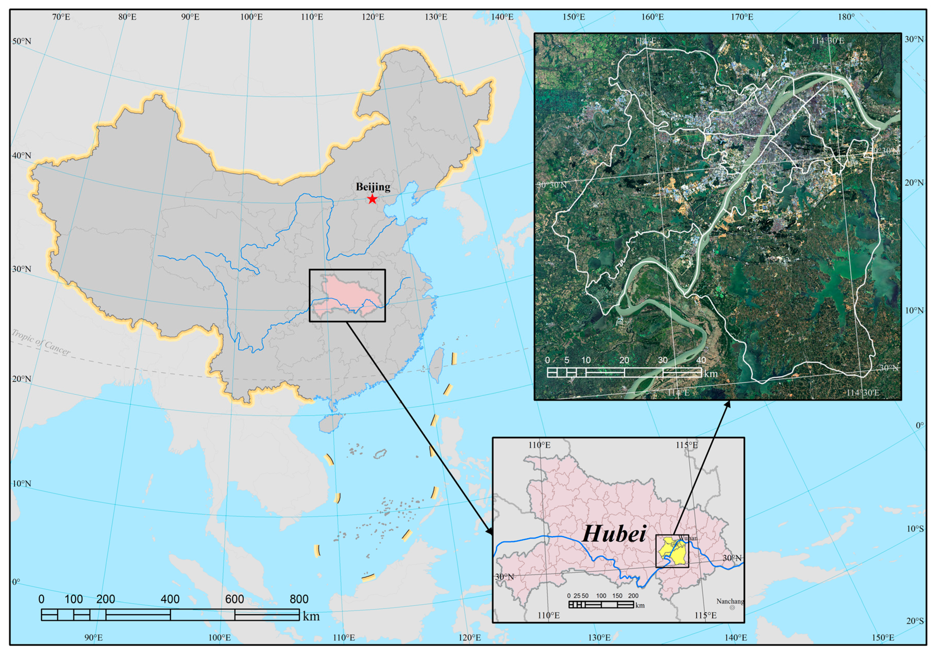
The study was conducted in Wuhan (113°41′E~115°05′E, 29°50′N~31°22′N), the capital of Hubei Province, located in central China and covering an area of 8494.41 km2 (Figure 1). Wuhan has a humid subtropical climate, with an annual total precipitation of 1315 mm and an annual mean temperature of 17.13 °C. Wuhan has a wealth of water and forest resources. It lies at the intersection of the Yangtze and Han rivers, and contains 166 lakes and over 70 parks. Its natural vegetation is composed primarily of deciduous broadleaf trees and evergreen broadleaf trees, such as camphor and oak. Evergreen needleleaf trees (e.g., Pinus massoniana Lamb) are also common in Wuhan, but they are sparsely mixed with broadleaf trees.
Wuhan is among the fastest growing cities in China, and has experienced rapid urban expansions in recent decades. The urban area in Wuhan increased from 4.19 × 10⁴ ha in 1988 to 49.39 × 10⁴ ha in 2011 [28], and the urban landscape became more fragmented. Wuhan comprises 13 districts with a total population of approximately 10.4 million. Our study area includes 11 districts, covering the whole metropolitan area and within one tile of Landsat images.
2.2. Data and Processing
2.2.1. Satellite Data and Products
In this study, 2576 eight-day MODIS composites (MOD09A1, from the Terra platform) from 2000 to 2013 were obtained from the Earth Observing System (EOS) data gateway (http://redhook.gsfc.nasa.gov) of the National Aeronautics and Space Administration (NASA). MOD09A1 has 500-m resolution and seven spectral bands, with each pixel containing the best observation during the eight-day period. Data were reprojected to the Universal Transverse Mercator (UTM) projection. For each date, four MODIS tiles (h26v05, h27v05, h27v06, h28v06) were mosaicked, and then clipped to the extent of the study area.
The absence of a flux tower around the study area made validations of GPP difficult. In this study, MOD17A2, an eight-day composite GPP product at 1-km resolution, was resampled to 30-m spatial resolution using the nearest-neighbor interpolation method. MOD17 is the GPP product computed with the MODIS land-cover (MOD12), MODIS Fraction of Photosynthetically Active Radiation/Leaf Area Index (FPAR/LAI) product, and Global Modeling and Assimilation Office (GMAO) surface meteorology for the vegetated land surface [13,29]. MOD17 has been validated in different ecosystems, showing a high correspondence with field measurements [29,30,31,32]. The resampled MOD17 GPP was used to validate the estimated GPP based on the pixels of the same land cover types in land cover maps derived from both Landsat images and MOD12 land cover data.
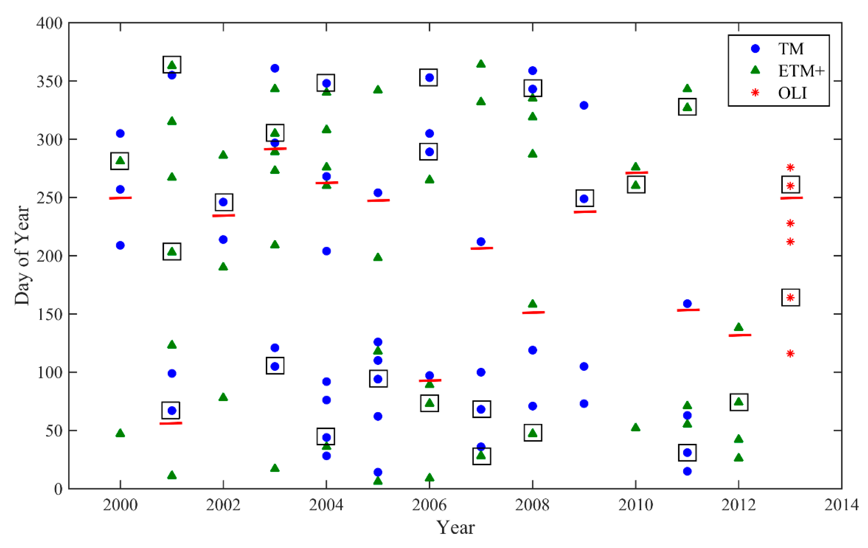
From 2000 to 2013, 99 Landsat surface reflectance images (path 123 row 039) with a cloud cover of less than 20% were downloaded from the United States Geological Survey (USGS) Earth Resources Observation Systems (EROS) data center, including 45 TM images, 48 ETM+ images, and six images acquired by Landsat-8 Operational Land Imager (OLI) (Figure 2). The scan line corrector (SLC)-off effect (which results in missing data lines in the image) was evident within some of the ETM+ scenes, and the missing data were filled with a gap-filling method [33]. For each year, one to three images were used to evaluate the accuracy of the STARFM-generated synthetic NDVI (referred to as the synthetic NDVI in the following text), and the rest of the available images were used as the inputs to the STARFM simulations. For the year 2009, since the available images were scarce, in order to maintain the quality of the synthetic NDVI, the selected image was used for both prediction and validation. In addition, the clearest image (cloud cover less than 10%) acquired between April and August was selected for each year to create the land cover map.
2.2.2. Meteorological Data
The daily meteorological data at 15 weather stations within and around the study area during 2000–2013 were used in this study. Meteorological data, including minimum temperature, relative humidity, and solar radiation, were obtained from the Chinese National Meteorological Information Center (http://data.cma.gov.cn). Vapor pressure deficit (VPD) was calculated from the relative humidity as:
where VP is the daily mean vapor pressure, and RH is the daily mean relative humidity [34].
VPD = VP × 100/RH − VP
The inverse distance weighting method was used to interpolate meteorological variables at 30-m spatial resolution. Daily meteorological data were then averaged for every eight days to estimate GPP in the study area.
3. Methods
3.1. Generation of the NDVI Time Series Using STARFM
STARFM produces a synthetic image based upon a spatially weighted difference computed between the Landsat and the MODIS scenes acquired at t1, and the Landsat t1-scene and one or more MODIS scenes of prediction day (t2), respectively [19]. The application of STARFM to ratio indices rather than reflectance usually provides more consistent indicators of vegetation, since normalization reduces the radiometric and atmospheric effects from different sensors [23,35]. We applied STARFM to MODIS and Landsat NDVI data, generating the synthetic NDVI time series with an eight-day interval and at 30-m spatial resolution. The time series of the NDVI was smoothed using the Harmonic Analysis of Time Series (HANTS) method [36].
To evaluate the accuracy of the synthetic NDVI generated by STARFM, we compared the synthetic NDVI against the NDVI derived from the original Landsat images in four test regions in the study area, with two regions in the homogeneous cropland, and two regions in the homogeneous evergreen broadleaf forest (EBF).
3.2. Creation of Land-Cover Maps
To parameterize the model to estimate GPP, the study area was classified into seven land-cover types, including EBF, deciduous broadleaf forest (DBF), grassland, cropland, built-up, bare land, and water bodies. In Wuhan, the needle tree is not the dominant tree type, and is usually mixed with broadleaf trees. Shrubs are mainly used to decorate roads. Thus, we excluded needle leaf forest and shrubs from our study, because it was difficult to accurately differentiate needle trees and shrubs from other vegetation types at 30-m resolution in the study area. Built-up areas, bare land, and water bodies were treated as non-vegetated areas.
Maximum likelihood classifier, a widely-used supervised classification approach, was employed in this study for the land-cover classification. Classification was conducted for each year on the selected image shown in Figure 2. Samples were collected for each image through the visual interpretation of Landsat images, with the help of a 2013 summer image of WorldView-2, higher resolution images in Google Earth, and field observations. A random stratification procedure was performed to generate training (80%) and testing (20%) datasets for each year. The NDVI values derived from Landsat images of different seasons were used to build a decision tree to classify forests into EBF and DBF.
3.3. Estimation of GPP
The GPP of urban vegetation was estimated using the MOD17 algorithm, which is based on the light-use efficiency (LUE) method [37]. GPP is related to the amount of photosynthetically active radiation (PAR) absorbed by the canopy through the use of a maximum radiation use conversion efficiency term (ε), such that [12]:
where fPAR is the fraction of incident PAR absorbed by the canopy, and PAR is the flux density of photosynthetically active radiation.
The value of ε depends on the vegetation type, and is reduced by the daily minimum air temperature (TMIN) and day-time vapor pressure deficit (VPD). ε is calculated as:
The lack of flux towers within or around the study area made it inapplicable to calibrate ε using field data. The parameters for calculating LUE were taken from the modified biome property look-up table (BPLUT) provided by Zhao and Running [38]. TMIN and VPD scalars are multipliers that reduce the conversion efficiency when cold temperature and/or high VPD inhibit photosynthesis. The scalars are calculated as follows:
where TMIN is the daily minimum temperature, TMINmin is the daily minimum temperature at which LUE is 0, and TMINmax is the daily maximum temperature at which LUE is maximum.
where VPDmin is the daily minimum VPD at which LUE is maximum, and VPDmax is the daily maximum VPD at which LUE is 0.
fPAR was calculated with STARFM-derived synthetic NDVI, using the equation proposed by Myneni and Williams [39]:
The GPP values of built-up areas, water bodies, and bare land within the study area were set to zero.
To minimize the effects of meteorological variations and emphasize the impacts of LUCC, GPP was estimated at 30-m resolution for every eight days under two scenarios. In the first scenario, GPP was estimated with the STARFM-generated NDVI, land cover maps, and ground-based meteorological measurements from 2000 to 2013. In the second scenario, GPP was estimated using the STARFM-generated NDVI from 2000 to 2013, the land cover maps from 2000 to 2013, and the meteorological data of the year 2000. The estimation of the first scenario (referred to as GPP_act) represented the actual dynamics of GPP in the study area, and was used for validation. The GPP estimated under the second scenario (referred to as GPP_ref) was used to quantify the impacts of LUCC on GPP in the urban areas.
3.4. Analysis of Impacts of LUCC on GPP
To take advantage of yearly land cover data, we quantified the relationship between the interannual variation of GPP_ref and that of the built-up, cropland, grassland, EBF, and DBF fraction, respectively, by calculating the Pearson correlation coefficient (r). The multiple correlation coefficient (R) was used to quantify the combined impacts of variations in multiple land cover types on GPP. The interannual variation of a variable was defined as the difference between the value of the current year and the value of the previous year. The yearly and multi-year cumulative transition matrixes of GPP_ref loss and gain associated with LUCC were computed for the study area.
Besides the widely used statistical methods, a change rate map was created to illustrate the spatiotemporal variations of GPP_ref caused by urbanization. To do so, a linear regression was performed over the annual GPP_ref values at each pixel, and the slope of the regression was used as the change rate of GPP at each location. The change rate showed the trend (positive/negative sign of the slope) and pace (magnitude of the slope) of the change in GPP over the study period.
4. Results
4.1. The Synthetic NDVI
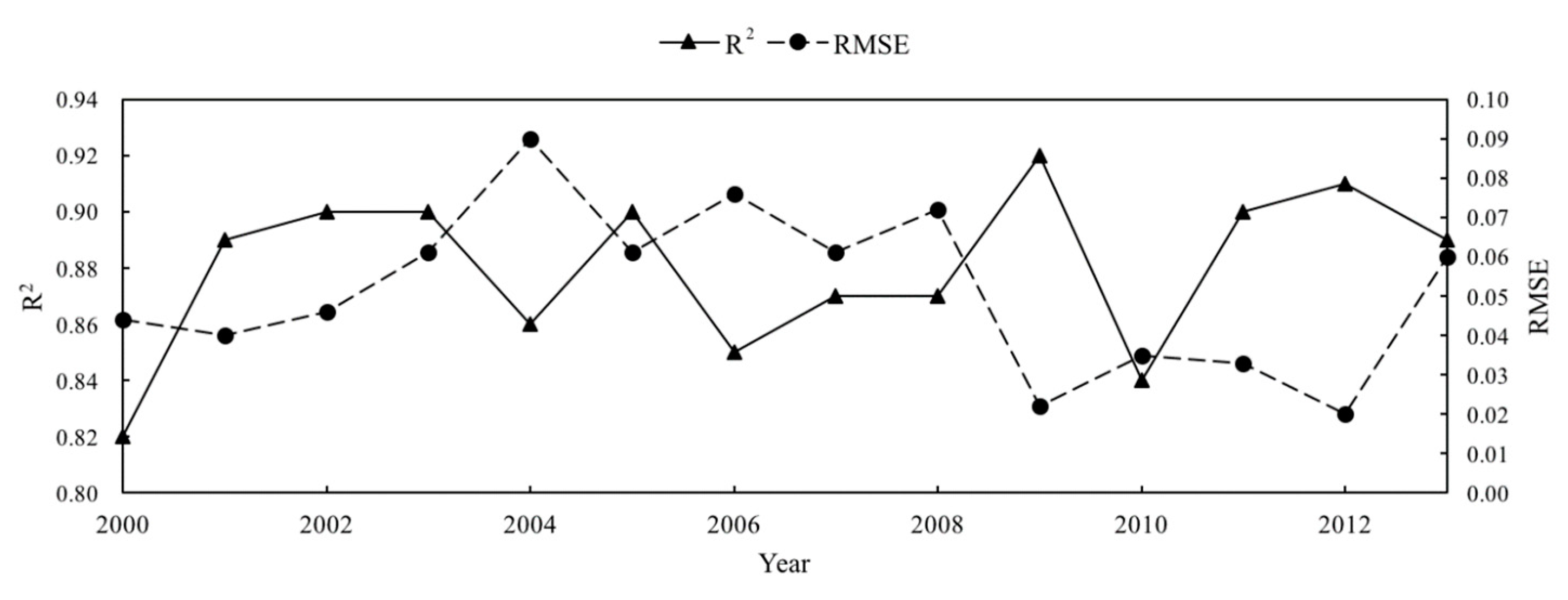
We assessed the accuracy of the synthetic NDVI in the four test regions for each year, using the independent Landsat images. The statistics shown in Figure 3 demonstrate that the synthetic NDVI has a close correspondence with the NDVI derived from the original Landsat images, with R2 ranging from 0.82 (p < 0.001) in 2000 to 0.93 (p < 0.001) in 2011, and a root mean square error (RMSE) ranging from 0.02 in 2012 to 0.09 in 2004.
4.2. Validation of GPP Estimates
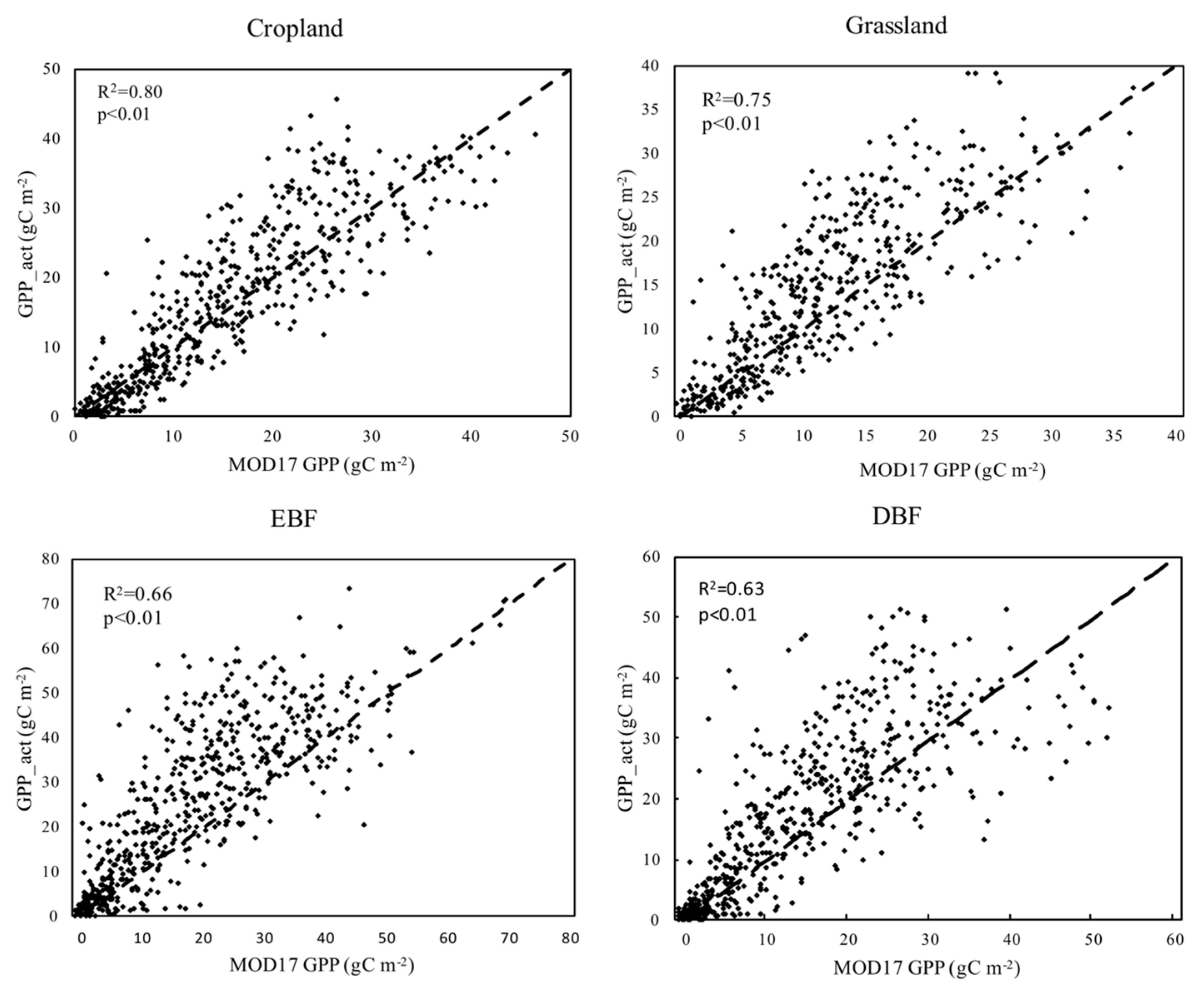
We roughly compared GPP_act with the results of Li et al.’s study [40], which predicted the GPP in China from 2000 to 2009 using the Eddy Covariance-Light Use Efficiency (EC-LUE) model, and validated results with measurements of 23 EC flux towers in China. Our estimates of different biomes were within the range of GPP observations shown in Li et al.’s study. Additionally, we compared our eight-day GPP estimates against MOD17 GPP for cropland, grassland, EBF, and DBF averaged on the pixels of the same land cover types on the land cover maps derived from both Landsat images and MOD12 land cover data. We found that GPP act was in agreement with MOD17 GPP for all of the vegetation types (Figure 4), but the values of GPP act were slightly higher than those of MOD17 GPP, especially for EBF and DBF.
4.3. LUCC in the Study Area
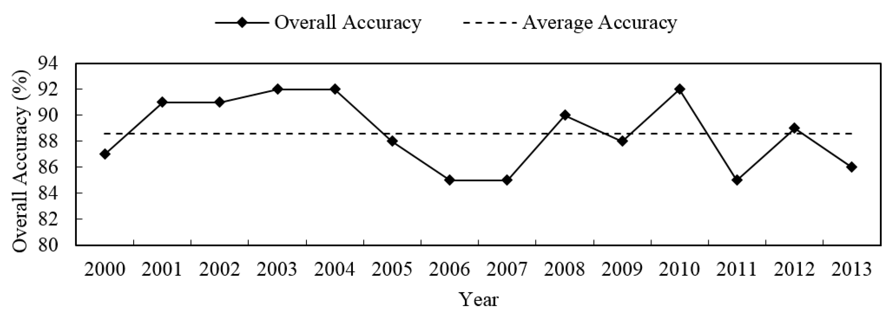
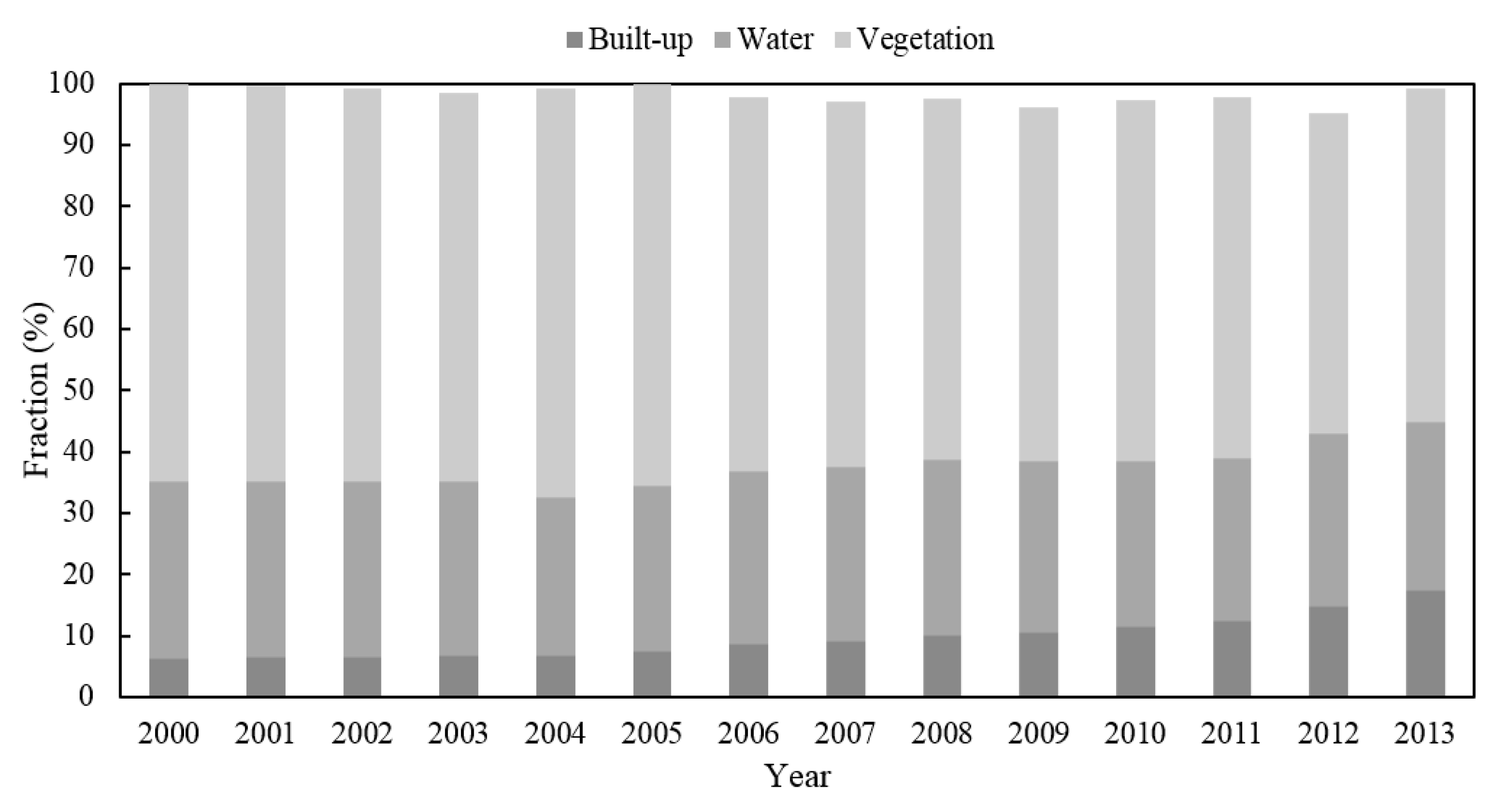
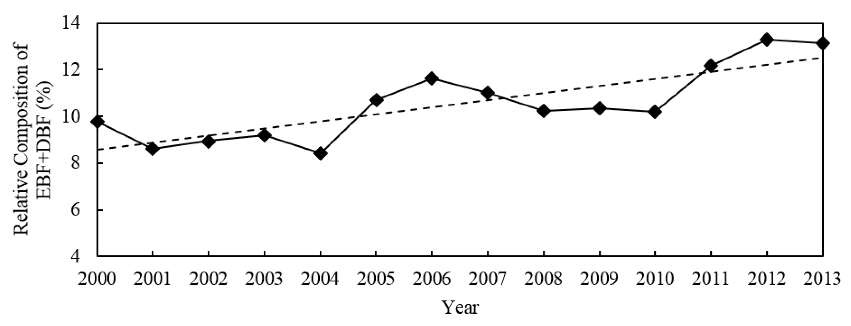
The overall accuracy of the land cover map for each year was evaluated with the testing samples, and is illustrated in Figure 5. The average accuracy of 14 years was 88.6%. Figure 6 summarizes the area fractions of built-up, water bodies, and vegetation (including grassland, cropland, EBF, and DBF) in the study area (bare land is not shown in Figure 6 due to the minimal area). It is evident that built-up areas increased rapidly after 2005, with an annual growth rate of 13.2%. On the other hand, vegetated area reduced by 0.9% per year, and water bodies decreased by 0.4% per year. While the total vegetated area was decreasing from 2000 to 2013, the fraction of forest increased slightly, which was highlighted on the plot of the relative composition of forest (Figure 7).
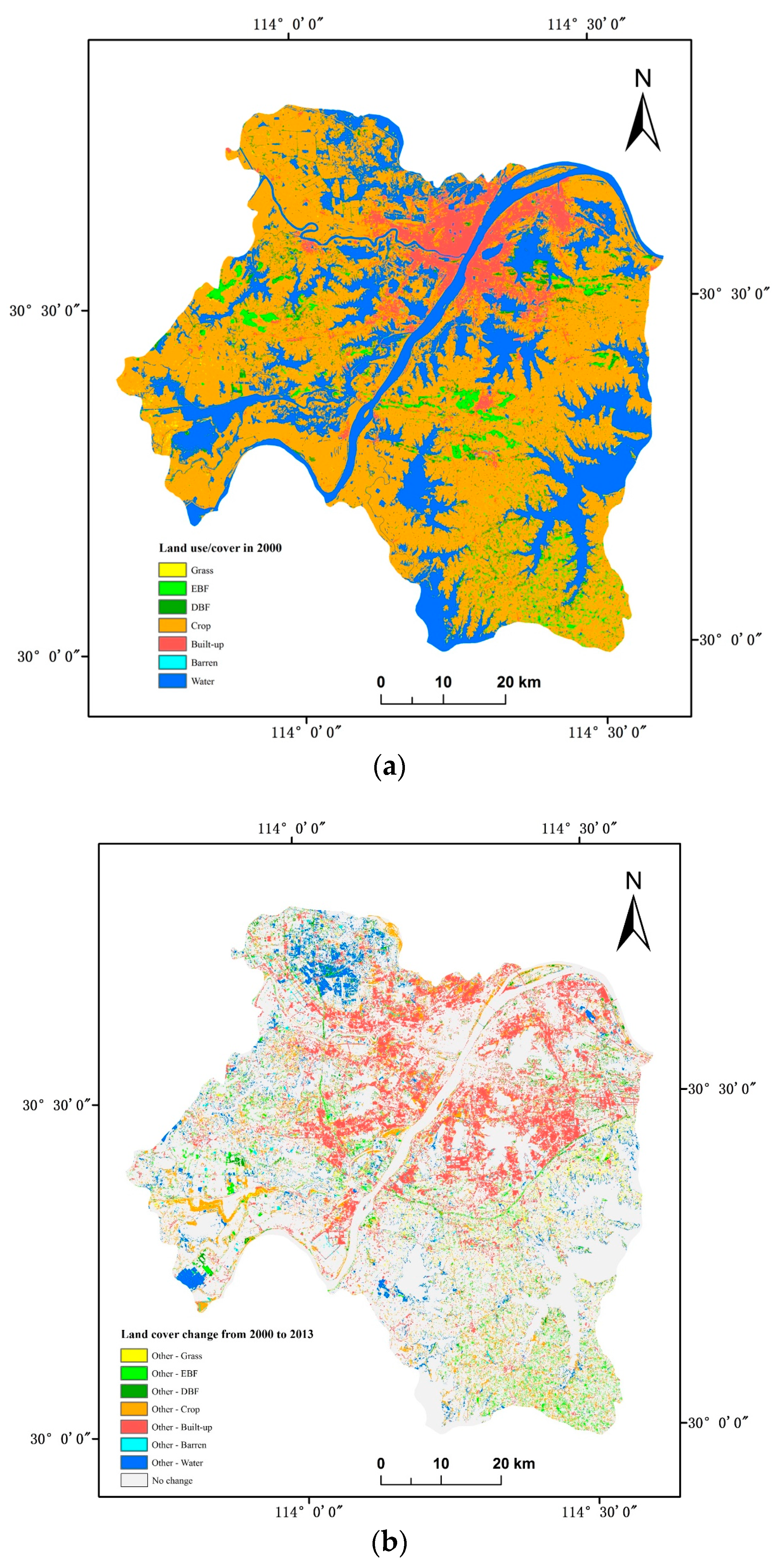
Figure 8 illustrates the spatial pattern of land-use/cover in 2000 and LUCC from 2000 to 2013 in the study area. The urban expansion resulted in the conversion of the large area of cropland in the suburb to built-up areas. The conversion from other land-use/cover types to water bodies can be found in the northwest of the study area, where areas of cropland were transformed to ponds in pursuit of higher economic benefits. The conversion from other land cover types to EBF or DBF primarily occurred in the southeast of the study area, where croplands were used to grow saplings.
4.4. Impacts of LUCC on GPP
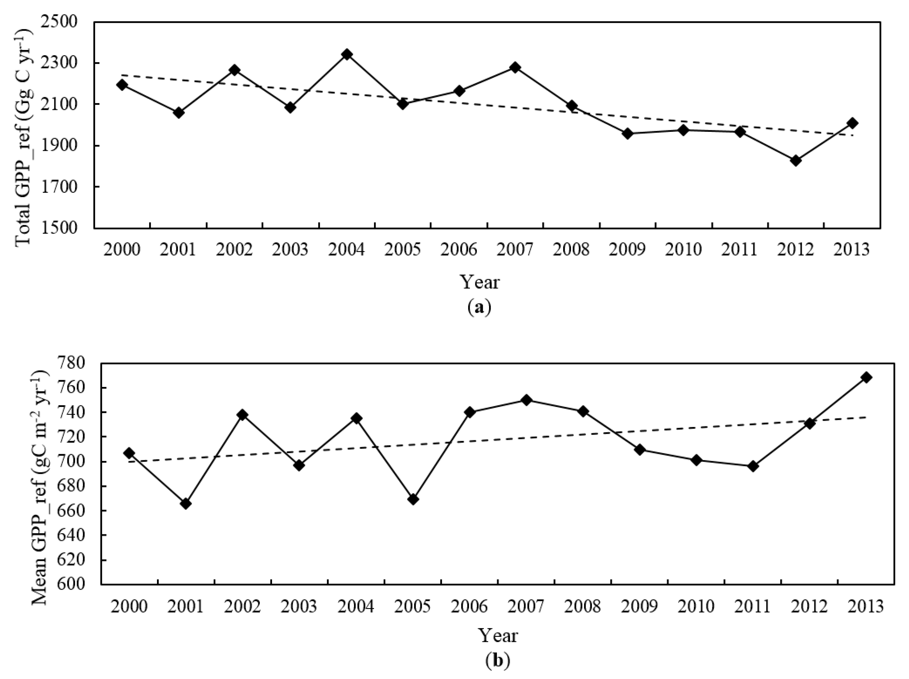
The temporal variations of GPP_ref over the study period were mainly controlled by LUCC, and the effects of meteorological variations had been largely minimized. Figure 9 illustrates the time series of the annual total GPP_ref and annual mean GPP_ref in the study area. The annual total GPP_ref showed a clear decreasing trend, with a decreasing rate of 1.02% per year (p < 0.1). The annual mean GPP_ref fluctuated from year to year, showing a weak increasing trend (p = 0.12).
We analyzed the relationship between the interannual variation of total GPP_ref and that of the built-up, cropland, grassland, EBF, and DBF fractions, respectively. The interannual variation of total GPP_ref had a negative linear relationship with the interannual variation of built-up fraction (r = 0.70, p < 0.05). During 2001–2005, when the pace of urbanization was slow, the interannual variation of GPP_ref was related to the interannual variation of the cropland fraction (r = 0.66, p < 0.05). During 2006–2013, when the built-up areas increased rapidly, the interannual variation of GPP_ref was related to that of the cropland fraction (r = 0.48, p < 0.1) as well as the forest fraction (r = 0.48, p < 0.1). The combined effect of changes in cropland and forest fraction on the interannual variation of GPP_ref can be quantified by the multiple correlation coefficient (r = 0.68, p < 0.05), implying that interannual variations in cropland and forest fractions together explained 68% variance in the interannual variation of GPP_ref.
We derived the transition matrix of the gain and the loss of annual GPP_ref associated with LUCC for each year in comparison with the annual GPP_ref of the previous year. The summary of the transition matrix over the 13 years is shown in Table 1. Besides the transition between cropland and bare land and the transition between cropland and water bodies, the maximum loss of GPP was associated with the conversion from cropland to built-up areas. The conversion from EBF and DBF to cropland and water bodies also contributed to a large amount of GPP loss. The substantial gain in GPP was due to the conversion from cropland to EBF and DBF. The transition between cropland and bare land may be caused by either crop rotation or urban expansion, with the net loss of 90.57 Gg C. The gain and loss of GPP that resulted from LUCC were not in balance. Approximately 309.95 Gg C in total was lost in the study area over the 13 years.
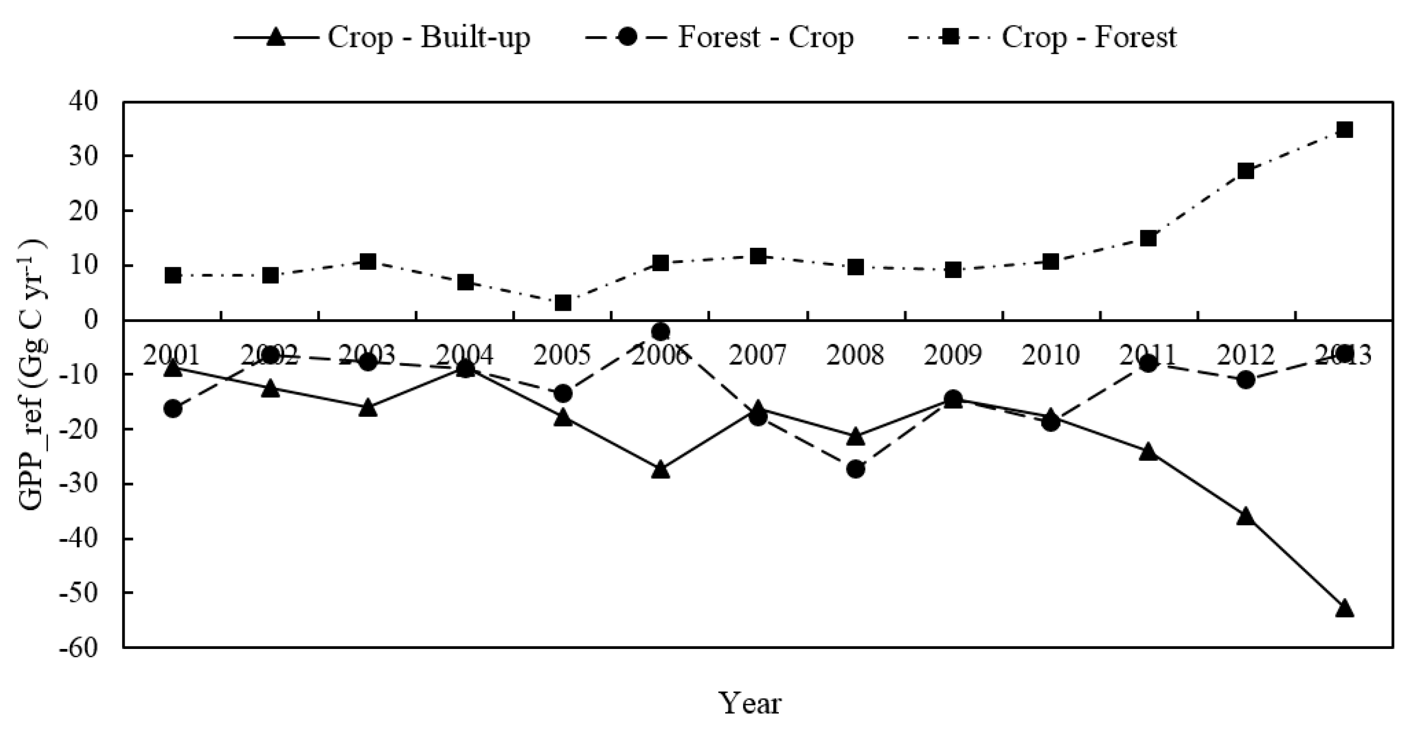
Figure 10 shows the temporal variations of loss and gain of GPP that was associated with a specific form of LUCC. The loss of GPP associated with the conversion from cropland to built-up areas increased slightly from 2001 to 2009, but the loss of GPP was worse after 2009, when built-up areas expanded rapidly. The loss of GPP due to the conversion from forest to cropland fluctuated through the study period, but it showed a sharp decrease in 2007 and 2008. The gain of GPP due to the conversion from cropland to forest was low during 2001–2009, but it increased dramatically from 2009 to 2013.
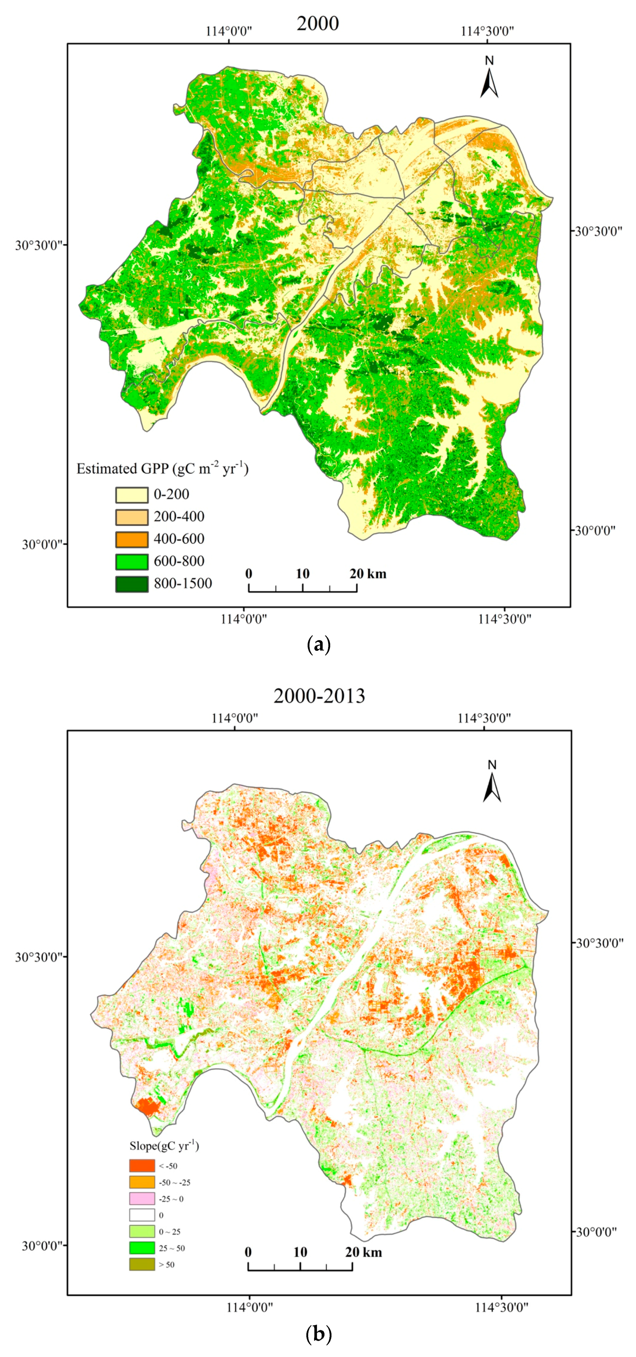
The spatial patterns of GPP_ref in 2000 is shown in Figure 11a. Urban forests showed the highest GPP values, and cropland in the suburb also had high GPP values ranging from 600 gC m−2 year−1 to 800 gC m−2 year−1. The medium GPP values (400–600 gC m−2 year−1) were found on the edge of the metropolitan areas or the water bodies, where land cover may change during the year. The slope of the linear regression on the time series of GPP_ref at each pixel served as the indicator of the change rate of GPP. The spatial pattern of the change rate shown in Figure 11b generally agrees with the LUCC map shown in Figure 8. The most prominent decreases in GPP occurred around metropolitan areas and a few water bodies, where cropland and forest were transformed into built-up areas. Significant decreases can also be found in the northwest of the study area, because cropland was transformed to ponds for aquatic plants and fisheries. Large areas of increases in GPP can be found in the southeast of the study area, where patches of cropland were transformed into forest. Interestingly, a significant increase in GPP throughout the 14 years can be found along the Huyu highway (through the central study area), along which the greenbelt was built around 2006.
5. Discussion
5.1. GPP Estimated at 30 m Spatial Resolution
While urban areas are highly fragmented and heterogeneous, most models simulate GPP in urban areas at coarse resolutions (e.g., 1–2 km) [5,6,7]. In this study, vegetation GPP in Wuhan was estimated at 30-m spatial resolution with land cover maps derived from Landsat images, the synthetic NDVI generated with STARFM, and meteorological measurements. It is worth mentioning that since the NDVI that was used to calculate fPAR in the GPP estimation reflected the combined effect of LUCC, meteorological variations and phenology, it was extremely difficult to completely eliminate the impact of meteorological variations on the GPP estimation.
The STARFM has been found to be able to produce an accurate interpolated NDVI time series in many studies [21,25]. In this study, the variations in the accuracy of the synthetic NDVI may be due to different atmospheric conditions when MODIS data and Landsat data were obtained on different days. GPP estimated with the synthetic NDVI demonstrated more spatial details and complexities in the urban area (Figure 11). The greater level of details provided a better representation of fringe areas and small LUCC than the models with 1–2 km spatial resolutions [26].
Directly validating GPP estimates in the urban area is difficult, due to the absence of EC flux towers in cities [7,10,41]. In this study, we proved the reliability of vegetation GPP estimates by comparing GPP_act with Li et al.’s [40] results and MOD17 GPP. Overall, values of GPP_act were within the reasonable range. The slightly higher values of GPP_act compared with the MOD17 GPP values were due to several factors. In the MOD17 GPP algorithm, fPAR was estimated with atmospherically corrected daily bidirectional reflectance and land cover classification [29], whereas GPP_act was based on the linear relationship between fPAR and NDVI. In addition, fPAR used in GPP_act was smoothed, free of peaks and valleys in the curve. In the mid-growing season of crops and EBF, the abrupt low values of MODIS fPAR may have great impacts on estimations of GPP. Another reason attributed to the difference between GPP_act and MODIS GPP may be the difference between the ground meteorological data used in GPP_act, and the GMAO surface meteorology used in MODIS GPP.
The study was based on the assumption that air pollutants did not affect the GPP of urban vegetation. Air pollutants originating in a city and transporting outside can adversely affect atmospheric chemistry, as well as the vegetation in that region [42]. Vegetation productivity in the urban area may decrease or increase, depending on the type of pollution and its effect on vegetation productivity [43]. Besides, the air temperature in the urban area may be more heterogeneous than air temperature that is estimated with observations at limited weather stations. Although the complex impacts of air pollutants and heterogeneous air temperature on vegetation GPP in the urban areas are very important issues, they are beyond the scope of this paper.
5.2. Impacts of LUCC on GPP
Wuhan is an excellent example of a human–natural system, where forests and wetland have been well preserved in recent decades as urbanization rapidly occurred. The results showed that in addition to the conversion from cropland to bare land and water bodies, the greatest loss of GPP was caused by the conversion from cropland to built-up areas that occurred in the suburbs and the exurbs due to urban expansion. This result was in agreement with findings reported by several studies that the substantial loss of primary production was due to the conversion from cropland to urban areas in the suburbs of cities in China [6,10]. Although built-up areas encroached cropland at a fast pace, the increasing relative fraction of forests that were more photosynthetically productive offset a certain amount of GPP loss. A study to analyze the impacts of LUCC on terrestrial carbon sinks and emissions in Guangzhou, China also reported that the carbon sink gained through the changes from the low carbon sink (e.g., grassland) to the high carbon sink (e.g., forests) [41]. Furthermore, they found that the proportion of urban land influenced the changes in carbon sinks, which is similar to our findings that the change in vegetation composition affected the interannual variation of GPP.
The conversion from cropland to water bodies led to a great loss of GPP that was even larger than the loss caused by the conversion from cropland to built-up areas. However, a certain amount of transition between cropland and water bodies may be due to the change from farmland to paddy fields, as the rotation between winter wheat/oilseed rape and paddy rice is common in the study area. Nonetheless, driven by economic benefits, the conversion from cropland to ponds for fisheries and aquatic plants led to the loss of GPP. Land cover maps were mostly derived from images of June, July, or August, but the date of the image used for classification varied from year to year. Hence, the transition between cropland and bare land may be either caused by the crop rotation or urban expansion.
The map of the GPP_ref change rate illustrates the spatiotemporal dynamics of GPP over 14 years. The significant decreases in GPP were found around the metropolitan area to be due to urban expansion, and around several major lakes because of the preferences of building apartments and houses near lakes and rivers. The greenbelt along the highway contributed to the interesting increasing trend in GPP. In the southeast of the study area, cropland was replaced by woods for economic reasons, leading to the increase in GPP. In the northwest of the study area, cropland was transformed to ponds, leading to the sharp decrease in GPP. The detailed map of the change rate demonstrated the ecological consequence of the characteristic land cover changes in a city.
China is currently promoting the concept of an urban ecosystem service [44]. In this study, the quantitative analysis of vegetation GPP changes over 14 years caused by LUCC may provide guidance to adjust land-use/cover structures in Wuhan in order to ensure minimized carbon loss in the future. Carbon consequences should be considered before land management policies and activities are put forth. Integrating more photosynthetically productive species in the limited area may largely mitigate the carbon losses that are associated with urbanization. Additionally, the method can be applied to other major cities, and combined with economic methods for policy-makers to establish carbon trading or offsetting rates policies [45].
6. Conclusions
This study quantified the impacts of LUCC on vegetation GPP during 2000–2013 in Wuhan, China at 30-m resolution, using yearly land cover maps derived from Landsat images, the synthetic NDVI generated by STARFM, and meteorological measurements. As the transition between cropland and water bodies or bare land was the combination of many factors, the greatest loss of GPP was due to the conversion from cropland to built-up areas, and the greatest gain of GPP was caused by the conversion from cropland to forests. Approximately 309.95 Gg C in total was lost in the study area during the 13 years. The interannual variation of GPP was mainly controlled by the change of cropland due to urban expansion, but the change in vegetation composition also affected the interannual variation of GPP. The loss of GPP due to the conversion from forests to cropland fluctuated throughout the study period, but it showed a sharp decrease in 2007 and 2008. The gain of GPP due to the conversion from cropland to forests was low during 2001–2009, but it increased dramatically from 2009 to 2013. The change rate map of GPP showed an interesting increasing trend along the highway, and a decreasing trend around the metropolitan area and lakes. The detailed maps of urban vegetation GPP in response to the rapid and fragmented LUCC facilitate the quantitative evaluation of the carbon consequences of land management activities and policies in urban areas. The results of this study suggested that the land-use/cover types should be adjusted wisely in urban planning in order to achieve the balance between the optimized economy and minimized carbon loss.
Acknowledgments
This research was supported by grants from the National Natural Science Foundation of China (Grant No. 41501367 and Grant No. 41671408). We acknowledge Feng Gao for making the STARFM code available. We thank Maosheng Zhao for his help with the MODIS GPP algorithm.
Author Contributions
Shishi Liu, Qingfeng Guan, and Shanqin Wang conceived and designed the experiments; Wei Du performed the experiments; Wei Du and Hang Su analyzed the data; Shishi Liu and Qingfeng Guan wrote the paper.
Conflicts of Interest
The authors declare no conflict of interest.
References
- Grimm, N.B.; Faeth, S.H.; Golubiewski, N.E.; Redman, C.L.; Wu, J.; Bai, X.; Briggs, J.M. Global change and the ecology of cities. Science 2008, 319, 756–760. [Google Scholar] [CrossRef] [PubMed]
- Li, F.; Wang, R.; Paulussen, J.; Liu, X. Comprehensive concept planning of urban greening based on ecological principles: A case study in Beijing, China. Landsc. Urban Plan. 2005, 72, 325–336. [Google Scholar] [CrossRef]
- Foley, J.A.; DeFries, R.; Asner, G.P. Global consequences of land use. Science 2005, 309, 570–574. [Google Scholar] [CrossRef] [PubMed]
- Milesi, C.; Elvidge, C.D.; Nemani, R.R.; Running, S.W. Assessing the impact of urban land development on net primary productivity in the southeastern United States. Remote Sens. Environ. 2003, 86, 401–410. [Google Scholar] [CrossRef]
- Imhoff, M.L.; Bounoua, L.; DeFries, R.; Lawrence, W.T.; Stutzer, D.; Tucker, C.J.; Ricketts, T. The consequences of urban land transformation on net primary productivity in the United States. Remote Sens. Environ. 2004, 89, 434–443. [Google Scholar] [CrossRef]
- Pei, F.; Li, X.; Liu, X.; Wang, S.; He, Z. Assessing the differences in net primary productivity between pre- and post-urban land development in China. Agric. For. Meteorol. 2013, 171–172, 174–186. [Google Scholar] [CrossRef]
- Buyantuyev, A.; Wu, J. Urbanization alters spatiotemporal patterns of ecosystem primary production: A case study of the Phoenix metropolitan region, USA. J. Arid Environ. 2009, 73, 512–520. [Google Scholar] [CrossRef]
- Xu, C.; Liu, M.; An, S.; Chen, J.M.; Yan, P. Assessing the impact of urbanization on regional net primary productivity in Jiangyin County, China. J. Environ. Manag. 2007, 85, 597–606. [Google Scholar] [CrossRef] [PubMed]
- Yu, D.; Shao, H.; Shi, P.; Zhu, W.; Pan, Y. How does the conversion of land cover to urban use affect net primary productivity? A case study in Shenzhen city, China. Agric. For. Meteorol. 2009, 149, 2054–2060. [Google Scholar]
- Fu, Y.; Lu, X.; Zhao, Y.; Zeng, X.; Xia, L. Assessment impacts of weather and land use/land-cover (LULC) change on urban vegetation net primary productivity (NPP): A case study in Guangzhou, China. Remote Sens. 2013, 5, 4125–4144. [Google Scholar] [CrossRef]
- Potter, C.S.; Randerson, J.T.; Field, C.B.; Matson, P.A.; Vitousek, P.M.; Mooney, H.A.; Klooster, S.A. Terrestrial ecosystem production: A process model based on global satellite and surface data. Glob. Biogeochem. Cycles 1993, 7, 811–841. [Google Scholar] [CrossRef]
- Running, S.W.; Thornton, P.E.; Nemani, R.; Glassy, J.M. Global Terrestrial Gross and Net Primary Productivity from the Earth Observing System. In Methods in Ecosystem Science; Sala, O.E., Jackson, R.B., Mooney, H.A., Howarth, R.W., Eds.; Springer: New York, NY, USA, 2000; pp. 44–57. [Google Scholar]
- Zhao, M.; Heinsch, F.A.; Nemani, R.R.; Running, S.W. Improvements of the MODIS terrestrial gross and net primary production global data set. Remote Sens. Environ. 2005, 95, 164–176. [Google Scholar] [CrossRef]
- Nightingale, J.M.; Coops, N.C.; Waring, R.H.; Hargrove, W.W. Comparison of MODIS gross primary production estimates for forests across the U.S.A. with those generated by a simple process model, 3-PGS. Remote Sens. Environ. 2007, 109, 500–509. [Google Scholar] [CrossRef]
- Sims, D.; Rahman, A.; Cordova, V.; Elmasri, B.; Baldocchi, D.; Bolstad, P.; Flanagan, L.; Goldstein, A.; Hollinger, D.; Misson, L. A new model of gross primary productivity for North American ecosystems based solely on the enhanced vegetation index and land surface temperature from MODIS. Remote Sens. Environ. 2008, 112, 1633–1646. [Google Scholar] [CrossRef]
- Gitelson, A.A.; Peng, Y.; Masek, J.G.; Rundquist, D.C.; Verma, S.B.; Suyker, A.; Baker, J.M.; Hatfield, J.L.; Meyers, T. Remote estimation of crop gross primary production with Landsat data. Remote Sens. Environ. 2012, 121, 404–414. [Google Scholar] [CrossRef]
- Lee, D.S.; Storey, J.C.; Choate, M.J.; Hayes, R.W. Four years of Landsat-7 onorbit geometric calibration and performance. IEEE Trans. Geosci. Remote Sens. 2004, 42, 2786–2795. [Google Scholar] [CrossRef]
- Wolfe, R.E.; Nishihama, M.; Fleig, A.J.; Kuyper, J.A.; Roy, D.P.; Storey, J.C.; Patt, F.S. Achieving sub-pixel geolocation accuracy in support of MODIS land science. Remote Sens. Environ. 2002, 83, 31–49. [Google Scholar] [CrossRef]
- Gao, F.; Masek, J.; Schwaller, M.; Hall, H. On the blending of the Landsat and MODIS surface reflectance: Predicting daily Landsat surface reflectance. IEEE Trans. Geosci. Remote Sens. 2006, 44, 2207–2218. [Google Scholar]
- Roy, D.P.; Ju, J.; Lewis, P.; Schaaf, C.; Gao, F.; Hansen, M.; Lindquist, E. Multi-temporal MODIS–Landsat data fusion for relative radiometric normalization, gap filling, and prediction of Landsat data. Remote Sens. Environ. 2008, 112, 3112–3130. [Google Scholar] [CrossRef]
- Hilker, T.; Wulder, M.A.; Coops, N.C.; Seitz, N.; White, J.C.; Gao, F. Generation of dense time series synthetic Landsat data through data blending with MODIS using a spatial and temporal adaptive reflectance fusion model. Remote Sens. Environ. 2009, 113, 1988–1999. [Google Scholar] [CrossRef]
- Gevaert, C.M.; García-Haro, F.J. A comparison of STARFM and an unmixing-based algorithm for Landsat and MODIS data fusion. Remote Sens. Environ. 2015, 156, 34–44. [Google Scholar] [CrossRef]
- Hwang, T.; Song, C.; Bolstad, P.V.; Band, L.E. Downscaling real-time vegetation dynamics by fusing multi-temporal MODIS and Landsat NDVI in topographically complex terrain. Remote Sens. Environ. 2011, 115, 2499–2512. [Google Scholar] [CrossRef]
- Walker, J.J.; de Beurs, K.M.; Wynne, R.H.; Gao, F. Evaluation of Landsat and MODIS data fusion products for analysis of dryland forest phenology. Remote Sens. Environ. 2012, 117, 381–393. [Google Scholar] [CrossRef]
- Schmidt, M.; Lucas, R.; Bunting, P.; Verbesselt, J.; Armston, J. Multi-resolution time series imagery for forest disturbance and regrowth monitoring in Queensland, Australia. Remote Sens. Environ. 2015, 158, 156–168. [Google Scholar] [CrossRef] [Green Version]
- Singh, D. Generation and evaluation of gross primary productivity using Landsat data through blending with MODIS data. Int. J. Appl. Earth Obs. Geoinf. 2011, 13, 59–69. [Google Scholar] [CrossRef]
- Churkina, G. Modeling the carbon cycle of urban systems. Ecol. Model. 2008, 216, 107–113. [Google Scholar] [CrossRef]
- Tan, R.; Liu, Y.; Liu, Y.; He, Q.; Ming, L.; Tang, S. Urban growth and its determinants across the Wuhan urban agglomeration, central China. Habitat Int. 2014, 44, 268–281. [Google Scholar] [CrossRef]
- Kanniah, K.D.; Beringer, J.; Hutley, L.B.; Tapper, N.J.; Zhu, X. Evaluation of Collection 4 and 5 of the MODIS gross primary productivity product and algorithm improvement at a tropical savanna site in northern Australia. Remote Sens. Environ. 2009, 113, 1808–1822. [Google Scholar] [CrossRef]
- Turner, D.P.; Ritts, W.D.; Cohen, W.B.; Gower, S.T.; Running, S.W.; Zhao, M.; Costa, M.H.; Kirschbaum, A.A.; Ham, J.M.; Saleska, S.R.; et al. Evaluation of MODIS NPP and GPP products across multiple biomes. Remote Sens. Environ. 2006, 102, 282–292. [Google Scholar] [CrossRef]
- Turner, D.P.; Ritts, W.D.; Zhao, M.; Kurc, S.A.; Dunn, A.L.; Wofsy, S.C.; Small, E.E.; Running, S.W. Assessing interannual variation in MODIS-based estimates of gross primary production. IEEE Trans. Geosci. Remote Sens. 2006, 44, 1899–1907. [Google Scholar] [CrossRef]
- Heinsch, F.A.; Zhao, M.; Running, S.W.; Kimball, J.S.; Nemani, R.R.; Davis, K.J.; Bolstad, P.V.; Cook, B.D.; Desai, A.R.; Ricciuto, D.M.; et al. Evaluation of remote sensing based terrestrial productivity from MODIS using regional tower eddy flux network observations. IEEE Trans. Geosci. Remote Sens. 2006, 44, 1908–1925. [Google Scholar] [CrossRef]
- Scaramuzza, P.; Micijevic, E.; Chander, G. SLC gap-filled products phase one methodology. Available online: https://landsat.usgs.gov/sites/default/files/documents/SLC_Gap_Fill_Methodology.pdf (accessed on 6 March 2018).
- Murray, F.W. On the computation of saturation vapor pressure. J. Appl. Meteorol. 1991, 6, 203–204. [Google Scholar] [CrossRef]
- Tian, F.; Wang, Y.; Fensholt, R.; Wang, K.; Zhang, L.; Huang, Y. Mapping and Evaluation of NDVI Trends from Synthetic Time Series Obtained by Blending Landsat and MODIS Data around a Coalfield on the Loess Plateau. Remote Sens. 2013, 5, 4255–4279. [Google Scholar] [CrossRef]
- Menenti, M.; Azzali, S.; Verhoef, W.; van Swol, R. Mapping agroecological zones and time lag in vegetation growth by means of fourier analysis of time series of NDVI images. Adv. Space Res. 1993, 13, 233–237. [Google Scholar] [CrossRef]
- Monteith, J.L. Solar radiation and productivity in tropical ecosystems. J. Appl. Ecol. 1972, 9, 747–766. [Google Scholar] [CrossRef]
- Zhao, M.; Running, S.W. Drought-Induced Reduction in Global Terrestrial Net Primary Production from 2000 through 2009. Science 2010, 329, 940–943. [Google Scholar] [CrossRef] [PubMed]
- Myneni, R.B.; Williams, D.L. On the relationship between FAPAR and NDVI. Remote Sens. Environ. 1994, 49, 200–211. [Google Scholar] [CrossRef]
- Li, X.; Liang, S.; Yu, G.; Yuan, W.; Cheng, X.; Xia, J.; Zhao, T.; Feng, J.; Ma, Z.; Ma, M.; et al. Estimation of gross primary production over the terrestrial ecosystems in China. Ecol. Model. 2013, 261–262, 80–92. [Google Scholar] [CrossRef]
- Xu, Q.; Yang, R.; Dong, Y.-X.; Liu, Y.-X.; Qiu, L.-R. The influence of rapid urbanization and land use changes on terrestrial carbon sources/sinks in Guangzhou, China. Ecol. Indic. 2016, 70, 304–316. [Google Scholar] [CrossRef]
- Crutzen, P.J. New directions: The growing urban heat and pollution “island” effect—Impact on chemistry and climate. Atmos. Environ. 2004, 38, 3539–3540. [Google Scholar] [CrossRef]
- Gregg, J.W.; Jones, C.G.; Dawson, T.E. Urbanization effects on tree growth in the vicinity of New York City. Nature 2003, 424, 183–187. [Google Scholar] [CrossRef] [PubMed]
- Li, Z.; Zhong, J.; Sun, Z.; Yang, W. Spatial Pattern of Carbon Sequestration and Urban Sustainability: Analysis of Land-Use and Carbon Emission in Guang’an, China. Sustainability 2017, 9, 1951. [Google Scholar] [CrossRef]
- Pearson, L.J.; Pearson, L.; Pearson, C.J. Sustainable urban agriculture: Stocktake and opportunities. Int. J. Agric. Sustain. 2010, 8, 7–19. [Google Scholar] [CrossRef]
Figure 1.
Location of the study area.

Figure 2.
The Landsat TM, ETM+, and OLI images used as the inputs to the STARFM simulations; images used for validations were marked with rectangles; images used for classifications were underlined.
Figure 2.
The Landsat TM, ETM+, and OLI images used as the inputs to the STARFM simulations; images used for validations were marked with rectangles; images used for classifications were underlined.

Figure 3.
The coefficient of determination (R2) and root mean square error (RMSE) of the relationship between the synthetic normalized difference vegetation index (NDVI) and the NDVI derived from the original Landsat images in four test regions in the study area (p < 0.001 for all of the studied years).

Figure 4.
Comparison of eight-day GPP_act against MOD17 GPP for cropland, grassland, EBF, and DBF. GPP were averaged on pixels of the same land cover type on land cover maps derived from both Landsat images and MOD12 land cover data.
Figure 4.
Comparison of eight-day GPP_act against MOD17 GPP for cropland, grassland, EBF, and DBF. GPP were averaged on pixels of the same land cover type on land cover maps derived from both Landsat images and MOD12 land cover data.

Figure 5.
The overall accuracy and the average accuracy of classification of Landsat images from 2000 to 2013. The maximum likelihood classifier was applied to classify seven land cover types in the study area.
Figure 5.
The overall accuracy and the average accuracy of classification of Landsat images from 2000 to 2013. The maximum likelihood classifier was applied to classify seven land cover types in the study area.

Figure 6.
Fractions of built-up, water bodies (Water), and vegetation (including cropland, grassland, EBF and DBF) in the study area from 2000 to 2013.
Figure 6.
Fractions of built-up, water bodies (Water), and vegetation (including cropland, grassland, EBF and DBF) in the study area from 2000 to 2013.

Figure 7.
The relative composition of EBF and DBF to the total vegetated area from 2000 to 2013. The dash line is the best-fit line of the linear regression, indicating the increasing trend of the relative composition of EBF and DBF through the study period.
Figure 7.
The relative composition of EBF and DBF to the total vegetated area from 2000 to 2013. The dash line is the best-fit line of the linear regression, indicating the increasing trend of the relative composition of EBF and DBF through the study period.

Figure 8.
The map of land-use/cover in 2000 (a); the map of land cover changes from 2000 to 2013 in the study area (b).
Figure 8.
The map of land-use/cover in 2000 (a); the map of land cover changes from 2000 to 2013 in the study area (b).

Figure 9.
Time series of the total annual GPP_ref (Gg C year−1) (a) and mean annual GPP_ref (gC m−2 year−1) (b) in the study area from 2000 to 2013. The dash lines represent the trends of the time series. The trend of the total annual GPP_ref was significant at p < 0.1; the trend of the mean annual GPP_ref was not significant (p = 0.12).

Figure 10.
Time series of gain and loss of GPP_ref associated with the conversion from cropland to built-up areas, the conversion from forest (including EBF and DBF) to cropland, and the conversion from cropland to forest (including EBF and DBF).
Figure 10.
Time series of gain and loss of GPP_ref associated with the conversion from cropland to built-up areas, the conversion from forest (including EBF and DBF) to cropland, and the conversion from cropland to forest (including EBF and DBF).

Figure 11.
The map of GPP_ref in the study area in 2000 (a); and change rate of GPP_ref from 2000 to 2013 (b). The change rate was calculated as the slope of the linear regression of the annual GPP_ref per pixel. The slope of the linear regression that was not significant (p > 0.1) was set to 0.
Figure 11.
The map of GPP_ref in the study area in 2000 (a); and change rate of GPP_ref from 2000 to 2013 (b). The change rate was calculated as the slope of the linear regression of the annual GPP_ref per pixel. The slope of the linear regression that was not significant (p > 0.1) was set to 0.


Table 1.
The cumulative gain (positive values) and loss (negative values) of the annual GPP_ref (Gg C) associated with land-use/cover change (LUCC) in each year from 2000 to 2013. Values smaller than 0.1 Gg C were set to 0.
Table 1.
The cumulative gain (positive values) and loss (negative values) of the annual GPP_ref (Gg C) associated with land-use/cover change (LUCC) in each year from 2000 to 2013. Values smaller than 0.1 Gg C were set to 0.
| Grass | EBF | DBF | Crop | Built-Up | Bare | Water | |
|---|---|---|---|---|---|---|---|
| Grass | 0 | −5.9 | −5.5 | −42.2 | 2.5 | 3.5 | 8.5 |
| EBF | 7.6 | 0 | 0 | 121.8 | 0.1 | 1.0 | 12.2 |
| DBF | 6.7 | 0 | 0 | 71.5 | 2.4 | 6.8 | 52.7 |
| Crop | 46.0 | −93.3 | −65.4 | 0 | 0 | 374.2 | 356.5 |
| Built-up | −8.3 | −0.7 | −17.1 | −272.8 | 0 | 0 | 0 |
| Bare | −5.9 | −1.6 | −13.2 | −464.7 | 0 | 0 | 0 |
| Water | −7.6 | −9.1 | −63.9 | −361.2 | 0 | 0 | 0 |
© 2018 by the authors. Licensee MDPI, Basel, Switzerland. This article is an open access article distributed under the terms and conditions of the Creative Commons Attribution (CC BY) license (http://creativecommons.org/licenses/by/4.0/).
Share and Cite
MDPI and ACS Style
Liu, S.; Du, W.; Su, H.; Wang, S.; Guan, Q. Quantifying Impacts of Land-Use/Cover Change on Urban Vegetation Gross Primary Production: A Case Study of Wuhan, China. Sustainability 2018, 10, 714. https://doi.org/10.3390/su10030714
AMA Style
Liu S, Du W, Su H, Wang S, Guan Q. Quantifying Impacts of Land-Use/Cover Change on Urban Vegetation Gross Primary Production: A Case Study of Wuhan, China. Sustainability. 2018; 10(3):714. https://doi.org/10.3390/su10030714
Chicago/Turabian StyleLiu, Shishi, Wei Du, Hang Su, Shanqin Wang, and Qingfeng Guan. 2018. "Quantifying Impacts of Land-Use/Cover Change on Urban Vegetation Gross Primary Production: A Case Study of Wuhan, China" Sustainability 10, no. 3: 714. https://doi.org/10.3390/su10030714
Note that from the first issue of 2016, this journal uses article numbers instead of page numbers. See further details here.