1. Introduction
Urban social and behavioral scientists have long been interested in
neighborhoods: what they are [
1,
2,
3,
4,
5,
6,
7]; how they form [
8,
9]; the processes by which they change over time, and, in turn, how those changes play out at higher levels of aggregation [
10,
11,
12,
13,
14,
15]; their roles in strategic planning and governance [
16,
17]; and, among other things, how (or if) they affect the behaviors and life outcomes of their constituent actors [
18,
19,
20,
21,
22,
23]. Concerning the latter of these themes, which is the focus of the current article, the ways in which neighborhood contexts influence individuals have proven quite difficult to study empirically. For, such inquiries must attend to a host of theoretical and methodological issues [
21,
22,
23,
24,
25,
26,
27].
Perhaps the most fundamental of these issues is what Kwan [
28] refers to as the “uncertain geographic context problem”, or UGCoP. Briefly, the UGCoP—which is distinct from the technically addressable modifiable areal unit problem [
28,
29]—describes the set of challenges associated with not knowing the “true” spatiotemporal context(s) that influences individual behavior (assuming that individual behavior is in fact influenced by contextual factors). In the absence of knowledge about such “behaviorally meaningful” geographies [
26], researchers are left to approximate neighborhood units in empirical analyses, frequently using areas delimited by straight line distances or administrative boundaries [
30]. However, there are few
a priori reasons to assume that these types of boundaries are causally relevant to an individual’s behavior ([
28,
29]; [
31], p. 134). To the contrary, they tend to be chosen for convenience with respect to data availability [
20,
21]. This means that the analytical units that regularly feature in quantitative neighborhood effects studies might, and presumably do, differ from actual spatial contexts that affect individuals. Such circumstances can produce spurious statistical associations between (misspecified) geographical contexts and individual behavior; or, they can lead to false negatives whereby “causally relevant” contexts do in fact influence individual behavior, but these effects are not detected by the misspecified models [
28,
29].
None of this is to say that extant scholarship on neighborhood effects which relies on administrative boundaries is unsound. In fact, this stream of literature has created a strong base of circumstantial evidence to suggest that individuals’ behaviors are indeed influenced by their spatial environments [
32,
33]. Nevertheless, in the context of the UGCoP, incautious assumptions that administrative boundaries adequately double as neighborhoods can lead to inferential errors [
28,
29]. Thus, it is useful for neighborhood effects researchers to begin their investigations by constructing well-grounded “conceptual model[s] that clearly specif[y] the causal pathways among contextual and outcomes variables”. This practice will aid in identifying “appropriate methods that can be used to better approximate the true geographic context[s] for the individuals being studied” ([
29], p. 249).
Toward these ends, this article argues that crossing relatively underexplored disciplinary boundaries can provide new insights for building the types of “sound conceptual models” that might currently be undersupplied in the prevailing neighborhood effects literature [
29]. In particular, recent research from the field of evolutionary studies is drawn on for its instructive work on conceptualizing and modeling neighborhood effects as
cross-level phenomena, whereby multiple, interacting spatial contexts influence individual behavior. These contributions guide the development of a statistical model that seeks to explain how individual property maintenance behavior in a selected U.S. study area changes as a function of neighborhood property conditions. Empirical tests of the model produce evidence suggestive of neighborhood effects operating at two interacting spatial levels that do not coincide with conventional administrative boundaries. While they are proffered as exploratory, these results nonetheless support the argument that interdisciplinary evolutionary research on social behavior can add value to studies of neighborhoods and neighborhood effects. That being said, to begin the investigation, it is necessary to briefly grapple with the idea of a “neighborhood” at a conceptual and operational level.
2. Conceptualizing and Operationalizing “Neighborhood”
In a special (neighborhood-themed) issue of
Urban Studies, Galster offers a parsimonious definition of
neighborhood: “a bundle of spatially based attributes associated with clusters of residences” ([
26], p. 2112). To the degree that the “geographic scale across which an attribute varies…is wildly dissimilar among attributes”, this definition suggests that the extent, boundaries, or even existence of a neighborhood depend on what attribute is being considered ([
26], pp. 2113–14). Put differently, the contextual or compositional dimension of interest (e.g., the amount of local demographic homogeneity; see [
4]) is itself what determines where and when a neighborhood exists [
26]. Interacting this observation with Galster’s [
8] concept of a “neighborhood externality space”, which is an “area over which changes in one or more
spatially based attributes initiated by others” alter the well-being of a given resident ([
26], p. 2114, emphasis added), a neighborhood comes to be seen as a
relation defined on a set of residences (see [
34]).
Grannis [
6] asserts that the specific relation of interest is “neighboring”. Neighboring, in turn, is a superposed relation that contains four levels, each of which necessarily follows from the one before (below) it. The foundational level of this relation—that on which all spatial neighborhoods are based—is geographic availability (“stage one neighboring”). Geographic availability is a function of relative, not absolute, proximity. When households are relatively proximate, actors are geographically available to experience passive contacts (“stage 2 neighboring”), passive contacts may then lead to intentional contacts (“stage 3 neighboring”), and intentional/active contacts can eventually produce mutual trust and a sense of community among neighbors (“stage 4 neighboring”) ([
6], pp. 17–19).
On that backdrop, where relative proximity of
residences behaviorally affects
residents, the trappings of a neighborhood are in place [
6]. Grannis argues that such situations very regularly manifest on one’s
face block [
6]. A face block “includes all of the dwellings that front…the same segment of the same street…between…two cross streets”. Within these spatial units, which terminate at street intersections, the probability of experiencing regular [at minimum] passive neighborly contacts is sufficiently high ([
6], pp. 31–33). More than this high probability of social contact, however, residents of the same face block are joint claimants on a collective good—a “neighborhood commons” [
35]. That is, while all residents of a face block enjoy the exclusive and rival use of the
interiors of their homes, the visible
exteriors of their homes, and the outdoor spaces and infrastructure that exist between them, are experienced and “used” collectively by all residents of the block. As a consequence, actions taken in this shared space—say, neglecting outdoor property maintenance and upkeep—affects the quality of the neighborhood commons for all residents of the block [
36]. This observation implies that face blocks are likely to be “behaviorally meaningful” [
26] and/or “causally relevant” [
28,
29] spatial contexts for a substantial fraction of the population.
Multiple Neighborhood Levels and Cross-Level Interactions
Importantly, face blocks rarely exist as islands that are closed off to other parts of human settlements. Thus, although face blocks constitute an intuitive and intimate spatial context that assumedly influences individual behavior [
6], they are only one of many possible geographic environments that perform this function [
28,
29,
33]. Acknowledging this point, many neighborhood effects studies in the social sciences have leveraged multilevel model specifications that classify observations into more than one (typically nested) group. For instance, persons might be grouped into households, with households grouped on face blocks, and face blocks grouped within, say, [clusters of] U.S. census tracts (e.g., [
21,
37]). Such model specifications allow researchers to “separately estimate the predictive effects of an individual predictor and its group-level mean”, where the latter are interpreted as contextual (
i.e., neighborhood) effects ([
38], p. 434). In this way, neighborhood effects can be detected at multiple levels in a spatial hierarchy [
37].
There is tremendous value in conceptualizing neighborhoods as multilevel entities [
39,
40], and in detecting their effects at multiple geographic levels [
21,
33,
37,
41]. Yet, while these objectives have received ample attention from social scientists in recent decades [
21], there has been comparably less effort aimed at detecting
cross-level interactions in contextual effects research [
41]. To articulate what is meant by “cross-level interactions”, this article adopts the definitions of the terms “level” and “scale” that are given in [
42]. Specifically,
scale refers to the “spatial, temporal, quantitative, or analytical dimensions used to measure and study any phenomenon”; and
levels are the “units of analysis…located at different positions on a scale” ([
42], p. 2). In other words, the
spatial scale consists of a continuous range of
levels including, for example, face blocks, cities, and regions [
42]. With that in mind,
cross-level interactions can be defined as “interactions among levels within a [spatial] scale” ([
42], p. 2).
Consider a case of two geographic
levels: (1) a face block and (2) the set of all face blocks connected to that face block by an intersection. The preceding section made the case that circumstances on one’s face block are likely to affect one’s behavior. Similarly, to the extent that “customary travel [is] one of the strongest influences” on an individual’s ability to mentally picture parts of a city ([
43], pp. 49–50), the face blocks that are directly connected to one’s own block—insofar as one or more of these streets needs to be accessed each time one travels outside of one’s immediate vicinity—plausibly structure at least part of an individual’s cognitive image of his or her “neighborhood” [
43]. Consequently, there is reason to believe that both of the aforementioned geographic levels are “behaviorally meaningful” [
26] and “causally relevant” [
28,
29] for a given individual.
If one assumes that contextual effects are present at both levels of this two-level schema, then a given individual’s “neighborhood context” can take on one of two qualitative states. First, the two spatial levels of the individual’s neighborhood may exhibit
congruence in the values of key contextual variables [
41]. In other words, the contextual attributes of the face block are the same as, or sufficiently similar to, the contextual attributes of the wider spatial environment that also includes all connecting face blocks. Second, the two levels may be
incongruent, or such that conditions on the given face block differ significantly from conditions on the surrounding face blocks [
41]. Whether the contextual effects associated with two (in)congruent spatial levels have reinforcing or balancing influences depends on the precise effects and behaviors under investigation. Hence, the nature of these effects ought to be engaged with at a conceptual level, prior to empirical analysis. That being said, neighborhood effects studies that do consider the possibility of cross-level interactions have done so: (1) via empirical models that hypothesize significant cross-level interactions in contextual effects, but that do not anticipate
ex ante the directions of these effects and (2) using administrative geographies, such as U.S. census block groups and municipal boundaries, as proxies for behaviorally meaningful spatial contextual levels [
41]. In response to these openings for further research, the remainder of this article: (1) draws on literature from evolutionary studies to construct a conceptual model that leads to testable hypotheses about the direction and nature of cross-level neighborhood effects and (2) in such a way that it grapples with the UGCoP. Concerning the latter, the empirical analysis forgoes reliance on comparatively arbitrary administrative boundaries to proxy for behaviorally meaningful or causally relevant neighborhood contexts.
3. Conceptual Model
A review of scholarship on the evolution of social structure is beyond the scope of this article, and interested readers can obtain a deeper understanding of this work from other sources [
44,
45,
46,
47,
48,
49]. For present purposes, consider only that evolution is a dynamic process in which individual-level variations have population-level consequences [
50,
51]. When variation in individual characteristics makes some actors better adapted to a shared environment than others, the frequency with which the “fitter” individuals’ characteristics occur in the overall population will increase with time [
47,
50,
51]. This observation sometimes leads to the misimpression that evolutionary processes disfavor cooperation among individuals—for, acting cooperatively tends to be costlier than free-riding on the efforts of others, which implies that non-cooperative strategies outcompete cooperative strategies in overall (randomly assorted) populations [
48]. Such scenarios are frequently portrayed in the context of a prisoner’s dilemma, wherein “defecting” strictly dominates (for any given individual) the strategy of “cooperating”. The implication is that cooperation is an unlikely population-level outcome [
45].
It is obvious, however, that cooperative social outcomes occur in the real world [
48,
50,
51,
52,
53]. One way that evolutionists explain this seeming inconsistency is by recognizing the important role of positive correlation in individual interactions [
44,
45,
49,
50,
51]. Namely, if cooperators are more likely to interact with other cooperators in a given environment than they are with defectors—
i.e., if cooperative behavior exhibits positive correlation—then cooperative outcomes can be locally adaptive [
45]. Moreover, if populations are positively assorted into spatial groups or neighborhoods, then the relative success of cooperative
groups in these configurations can bring about population-wide cooperation [
54,
55,
56]. An observable implication here is that non-cooperative behaviors make individuals relatively worse off when they live within a sufficiently high concentration of cooperators [
44,
46,
48]. By the same token, being a cooperator in a neighborhood of all defectors puts the prosocial minority at a distinct (relative) disadvantage [
54]. Accordingly, individuals tend to adjust their behaviors to make themselves at least as successful as other members in their reference groups—e.g., defectors living among all cooperators begin to cooperate [
36]. In familiar terms, individuals in these evolutionary models are subject to “neighborhood effects” ([
44], p. 24). Features from evolutionary models might therefore apply more generally to examinations of contextual influences in the social sciences.
To support this claim, insights from evolutionary studies are used here to create a conceptual model in which neighborhood effects are both multi- and cross-level. Explicitly, Skyrms [
44] describes a model that features what he calls geographically nested “imitation” and “interaction” neighborhoods. In this two-level spatial environment, cooperation spreads via imitation in a given locale when non-cooperative agents interact with sufficiently many cooperators in their immediate neighbor networks. However, the strength of this imitation effect is conditioned by the (non-)cooperation norms that prevail in a wider spatial context that contains, and extends beyond, both the given individual and the nearest neighbors whose behavior that individual is inclined to imitate. More precisely, the norms that prevail in an individual’s comparatively inclusive “interaction neighborhood” modify the probability with which he or she copies the behavior(s) of actors living in his or her more intimate “imitation neighborhood” [
44].
To help clarify these abstract concepts, consider that an
imitation neighborhood might consist of the set of households on one’s face block, as argued above in
Section 2. An
interaction neighborhood might then extend beyond the face block to include, for instance, all of the households on one’s face block,
plus all of the households on face blocks that share a street intersection with the given face block (refer to
Section 2) [
6]. In the interest of tractability, the remainder of this article refers to Skyrms’ [
44] higher resolution
imitation neighborhoods as a “level-1 neighborhoods”, and the lower resolution
interaction neighborhoods as a “level-2 neighborhoods”. Hence, all that readers must remember is that, as one is smaller than two, level-1 neighborhoods are geographically smaller (more compact and localized) than level-2 neighborhoods.
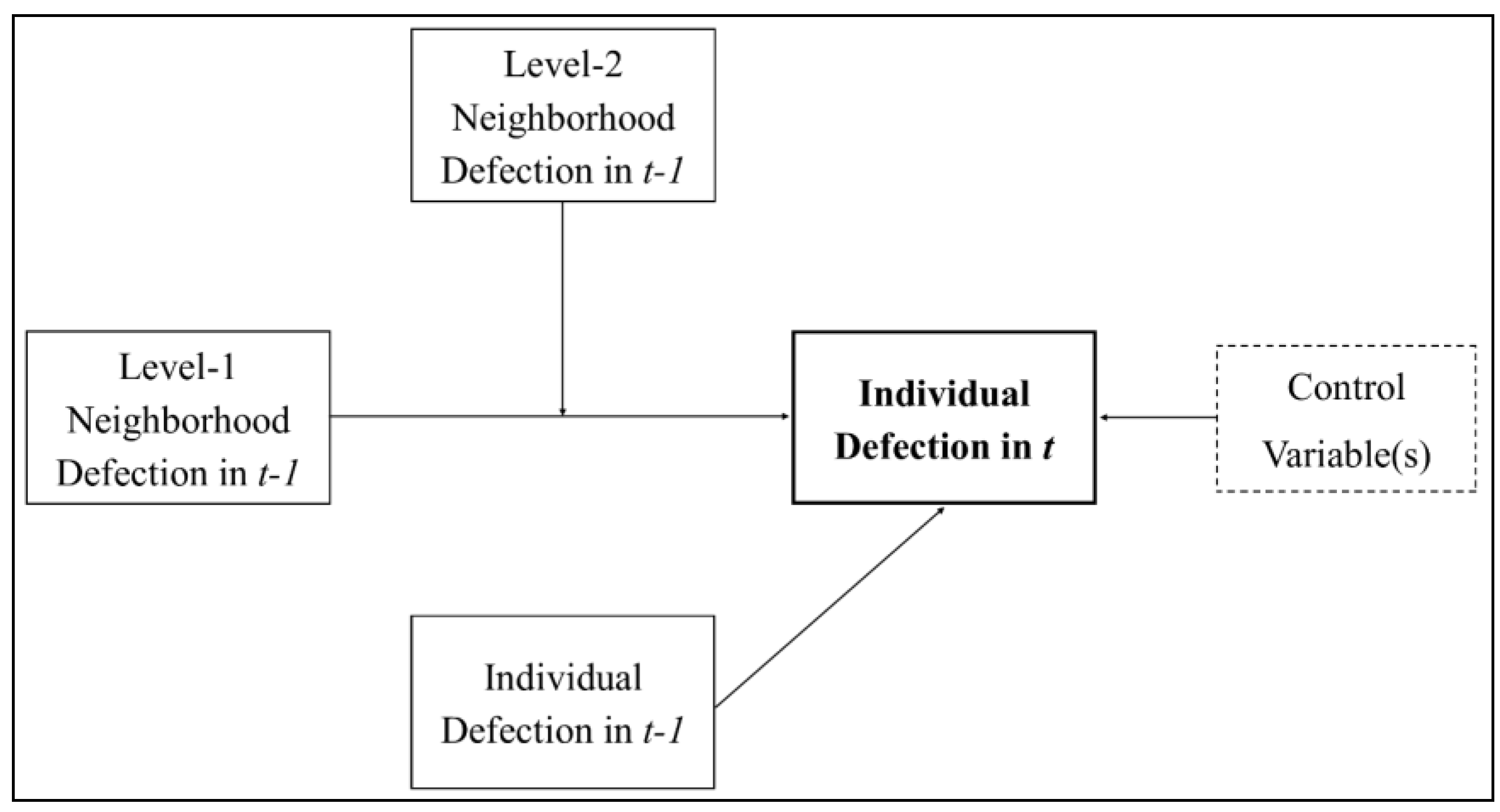
With the preceding definitions in hand,
Figure 1 proposes a general conceptual model of how individual-level defection (or cooperation), broadly defined, is influenced by local context in a two-level environment similar to the one described by Skyrms [
44]. In any given time period,
t, the probability that an individual engages in some antisocial or non-cooperative behavior depends on that individual’s behavior in an earlier time period,
t-1. This is a straightforward expectation which acknowledges that individuals are likely to exhibit similar behavioral tendencies across time [
57]. More interesting is the model’s hypothesized neighborhood effects. Namely, defection (or cooperation) is assumed to be directly influenced by one’s level-1 neighborhood context. That is, one is prone to conform to the behaviors of his or her nearest and most frequent interactants. However, the magnitude of this relationship is expected to change based on the wider geographic context in which one’s level-1 neighborhood is embedded, and in which one regularly observes local descriptive norms. Put another way, the influence that actions taken within one’s level-1 neighborhood have on one’s own behavior is
moderated by the context of one’s level-2 neighborhood. The probability that an individual imitates the (non-)cooperative behavior(s) of his or her neighbors is therefore not a constant property of a spatial system—it varies with geographic variation in level-2 social norms. While other neighborhood “levels” are most certainly relevant to an individual’s behavior, only two are considered here for parsimony.
Figure 1.
A two-level model of neighborhood effects with cross-level interactions.
Figure 1.
A two-level model of neighborhood effects with cross-level interactions.
4. Hypotheses, Data, and Methods
Cross-level neighborhood effects models like the one proposed in
Figure 1 are regularly tested in the evolutionary literature by simulating outcomes of hypothetical interactions on imaginary rectangular lattices [
44,
46,
48]. In contrast, the model in
Figure 1 is tested here for a real world case to explore the influences that substandard property conditions have on individual behavior in a selected city: Buffalo, NY, USA. Property conditions are of interest inasmuch as they are a decisive “spatially based attribute” (see
Section 2) for demarcating residential neighborhoods or housing submarkets [
11,
12,
14]. This is not to say that property conditions are the
exclusive spatially based attribute for defining neighborhood contexts and studying neighborhood effects. The variable is merely one important attribute that can be measured, and thus it can be used to explore the implications of the conceptual model in
Figure 1. On that note, property conditions in the selected study area are measured with parcel-level data on local property code compliance. Because property codes specify the minimum standards to which a built structure must legally be maintained, violation of these codes is an indicator of substandard conditions [
58]. In this sense, property code violation is effectively a non-cooperative social behavior (defection), while compliance is a cooperative behavior. In what follows, therefore, “violation” and “defection” (refer to
Figure 1) are used interchangeably, as are “compliance” and “cooperation”.
That being said, it is necessary to caution that code violations are an imperfect measure of defection of or cooperation with neighborhood property maintenance norms. Property inspections institutions tend to be complaint-driven, and they are embedded within local sociopolitical and cultural environments [
58]. Both of these points suggest that patterns of property code violations are observable outcomes of complex processes that cannot be adequately modeled using readily available micro-level data. For instance, the
Appendix shows that property code violations, when aggregated to the U.S. Census block group level (
i.e., an administrative geographic unit for which data are readily accessible), appear to vary systematically with: (1) local median home value; (2) local conditions of poverty; (3) average education levels; and (4) racial diversity. The former three variables speak to the intuitive notions that property upkeep is likely to correlate with both higher residential property values and economic advantage [
36]. The fourth variable supports Putnam’s [
59] highly-cited finding that ethnic diversity erodes social cohesion and cooperation. The upshot is that, while these four, and potentially many other, variables are probably involved in the processes that generate patterns of property code violations, they are typically only observable at administrative geographic levels. And, as argued above, assuming that measures taken from administrative geographic units have “causal relevance” for micro-level behavior is problematic in the context of the UGCoP [
28,
29]. For that reason, the analyses presented in this article rely exclusively on variables that can be measured for the individual and neighborhood levels that follow from the article’s
a priori engagements with the UGCoP (see
Section 2,
Section 2.1, and
Section 4.2). Because this choice necessarily omits relevant (but unmeasurable) variables from consideration, both the forthcoming analyses and the results obtained therefrom are proffered as exploratory, and intended only to test the implications of the model in
Figure 1 using real world data.
Minding these caveats, code violations are arguably one of the more relevant outcome variables that can be accessed with secondary data sources—at the resolution of an individual parcel—in pursuit of this article’s objectives. Indeed, the data obtained for this project were acquired at no financial cost through public information requests. Future studies with access to funding for primary data collection—in which more finely-tuned and customizable outcome and explanatory variables can be measured—will add significant value to this work.
4.1. Hypotheses
Prior to discussing the data available for this project in greater detail, it is necessary to convert the relationships from
Figure 1 into testable hypotheses. At the simplest level for chosen the empirical application, the model claims that an individual’s likelihood of violating the city’s property code in time
t is a function of (1) the individual’s property code violation behavior in
t-1, and (2) the
t-1 violation rate in the individual’s level-1 neighborhood. It is straightforward to hypothesize that these two explanatory variables will have direct relationships with the dependent variable, which is the probability that an individual defects in time
t. To make things slightly more complicated, however, the latter relationship is expected to manifest differently in different level-2 neighborhood contexts. In order to construct an informed hypothesis about this effect, it is useful to once again consult the evolutionary literature which guided development of the underlying conceptual model.
Instructive evolutionary models of social structure imply that an individual is likely to imitate the behaviors of his or her neighbors when those neighbors are successful “mutants” or “invaders” in the local environment—that is, when their behavior deviates from local norms in ways that increase their adaptedness to the environment relative to the given individual [
44,
46,
48]. This observation implicates a specific hypothesis about the moderated relationship shown in
Figure 1. Namely, in highly cooperative level-2 neighborhoods, violating is essentially a “mutant” behavior: the extant descriptive norm in cooperative neighborhoods is property code compliance. Consequently, in cooperative settings, an increase in the violation/defection rate in one’s level-1 neighborhood is likely to amplify the degree to which a given property owner violates the property code. The rationale is that free-riding level-1 neighbors do not incur the costs of cooperation, but they still enjoy the benefits of living in a cooperative level-2 neighborhood. With this line of reasoning in place, one is left with three testable hypotheses. The probability that an individual in the selected study area violates property code regulations in time
t:
- (1)
is higher for individuals who violated the property code in time t-1;
- (2)
increases as a direct function of the individual’s level-1 neighborhood violation rate; but such that;
- (3)
this “neighborhood effect” is amplified in cooperative level-2 neighborhoods (and, by extension, is muted in non-cooperative level-2 neighborhoods).
Given the above, the outstanding task is to operationalize level-1 and level-2 neighborhoods in a way that engages with the UGCoP. To proceed in that direction, the next section introduces the data available for this project.
4.2. Data
Data for the street addresses associated with all outstanding property code violations in Buffalo, NY were obtained through a public information request to the city’s Department of Management Information Systems. The request produced records for all unresolved property code violations through the end of the second quarter in 2009 [
60]. These records were batch geocoded in Esri ArcGIS 10.2 with a success rate exceeding 95 percent. The matched records were then joined to their respective real property tax parcels in a Geographic Information System (GIS). By joining the micro-level property code data to a geographic parcel dataset acquired from the city’s Office of Strategic Planning, every parcel in the study area can be coded as either cooperative (
i.e., not associated with a violation) or non-cooperative (
i.e., associated with a violation) during a given year. The dependent variable is then operationalized using the most recent observations (2008–2009) from the dataset. In turn, it is possible to calculate the fraction of a property’s neighbors who were violators prior to the focal year (
i.e., pre-2008–2009).
To facilitate this calculation, U.S. Census TIGER/Line shapefiles for 2010 were used to construct face blocks from the Census Bureau’s spatial data on all streets in Buffalo (refer to
Section 2) [
61]. Upon joining all parcels from the citywide parcel dataset to their respective face blocks in a GIS, the number of parcels on each face block was summed, and a minimum threshold of three “neighbors” was used to retain or exclude parcels from the sample. Parcels situated on face blocks with fewer than three total parcels were dropped from the sample. This step was taken to ensure that each parcel (owner) in the analysis was part of a
social environment, where sociologists and network theorists claim that social networks, and societies more generally, require at least three agents to exist [
62]. From there, the fraction of parcels with outstanding code violations was quantified for (1) each parcel’s face block, and (2) the total of the parcel’s face block and all of the face blocks with which the given block shares a street intersection. In this manner, each observation in the dataset is connected to
parcel-specific level-1 and level-2 neighborhoods. Moreover, the particular geographies used to operationalize these parcel-specific level-1 and level-2 neighborhoods follow directly from the engagements with the UGCoP that can be found earlier in this article (
Section 2).
4.3. Methods
The three hypotheses enumerated in
Section 4.1 can be tested in a regression model with interaction effects [
41,
63]. Namely, if the hypotheses are suitable, then performing a regression of individual-level violation behavior in
t on the (1) level-1 neighborhood violation rate in
t-1, (2) level-2 neighborhood violation rate in
t-1, and (3) product of (2) and (3), ought to produce statistically significant nonzero coefficients on all three of these terms [
41,
63]. This statement effectively describes a space-time regression model in which the dependent variable is explained by a time-lagged measure of itself at both neighborhood and individual levels [
36,
64]. Because violation behavior is binary coded, a limited dependent variable regression method, such as logit, is the appropriate modeling choice. The resulting empirical model takes the following form:
where
is the observed dichotomous dependent variable that takes on a value of 1 if individual
i defected in period
t and a value of 0 otherwise,
is the fraction of violators observed for
i’s face block in period
t-1,
is the fraction of violators observed for
i’s face block and connected face blocks during period
t-1, and
Ownership is a measure of housing tenure. More specifically with respect to the latter variable, in the context of O’Brien’s [
65] finding that homeownership increases cooperative property maintenance behavior in cities, the
Ownership variable takes on a value of 1 if a given parcel is estimated to be owner-occupied and a value of 0 otherwise. Values for this variable are estimated using the procedure described in [
65], which entails identifying exact matches in Buffalo’s geospatial parcel dataset between a parcel’s physical address and its owner’s mailing address. This imputed ownership predictor is expected to take on a highly significant and negative relationship with the violation dependent variable [
65,
66].
Next, recall that the code violation dataset does not completely cover the most recent year of data (see [
60]). As such, the dependent variable is measured for the partial year of 2009
plus the most recent full year of data. This choice has the added benefit of increasing variation in the dependent variable [
67]. That being said, because the code violation dataset describes outstanding violations,
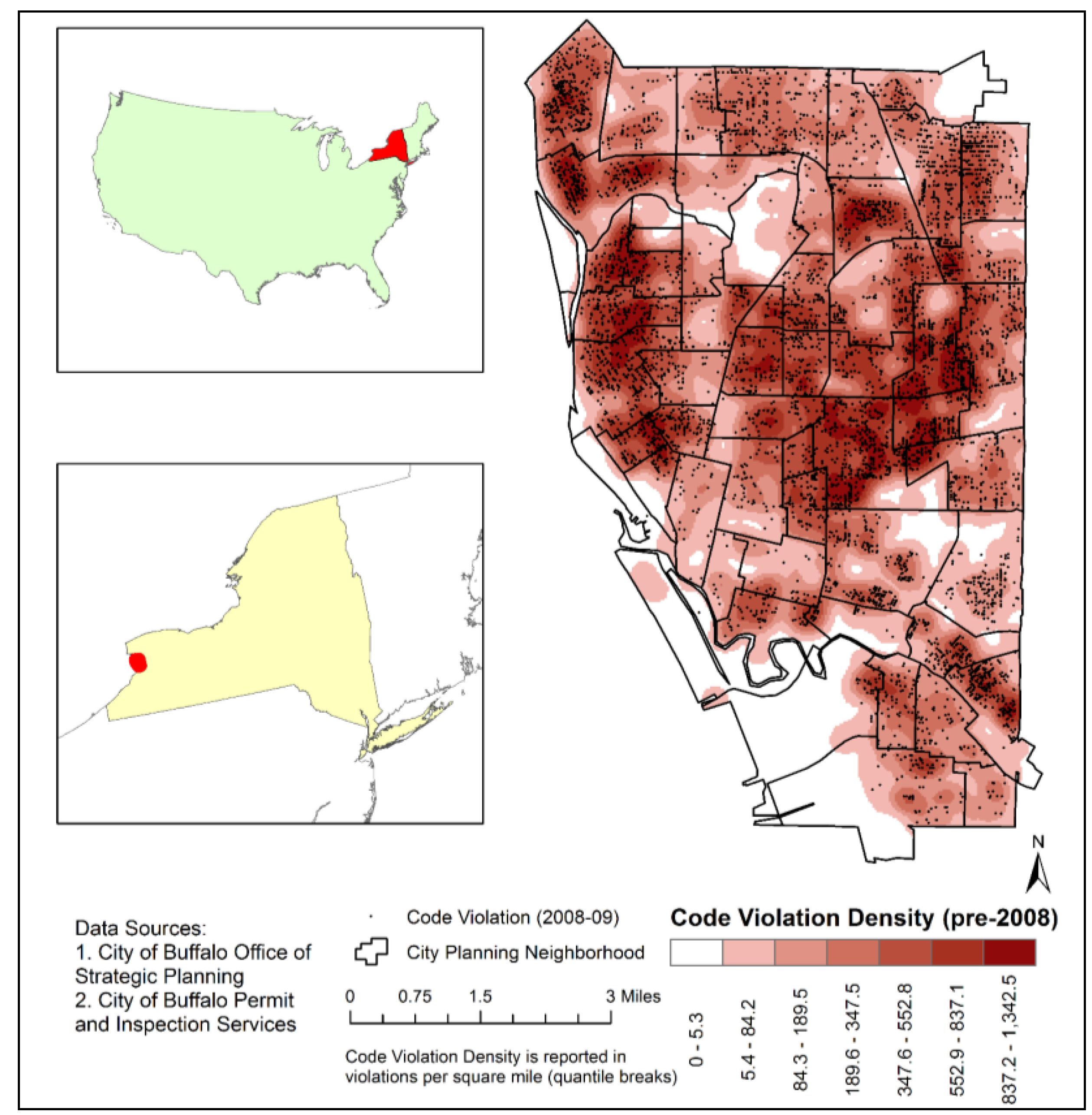
t-1 is set to include all violations that were unresolved (still present) on 31 December 2007, regardless of the date on which they were first recorded. The distributions of these two measures are mapped in
Figure 2, which depicts the density of outstanding pre-2008 violations relative to the locations of violations committed in 2008–2009.
Finally, consider that the number of property violations observed in 2008–2009 (
q = 6130) is small relative to the total number of parcels included in the citywide GIS dataset (
N = 90,614) (NB:
N excludes parcels that are situated on face blocks with fewer than three total parcels). To compensate for this disparity, estimation of the statistical model is carried out with the prior correction rare events logit (relogit) model proposed by King and Zeng [
68]. This method corrects for rare events bias in the model through its intercept, based on the population violation rate. Because the population rate in this case is known (
q/
N ≈ 7 percent), the relogit model allows the author to decrease the large number of non-violators (
M = 84,484) in the dataset in order to increase efficiency in carrying out the analysis [
68]. Accordingly, a random sample of
m = 6130 non-violators was taken and combined with the
q = 6130 violators to form an analytical sample of
n = 12,260. The reduced number of observations decreases computing time and virtual memory requirements, while insuring against rare events bias by adjusting the intercept of the model to account for the known population violation rate of approximately seven percent [
68].
Table 1 presents descriptive sample statistics for these data.
Figure 2.
Distribution of violations in the study area.
Figure 2.
Distribution of violations in the study area.
Table 1.
Characteristics of sample data.
Table 1.
Characteristics of sample data.
| Variable | Mean | Standard Deviation |
|---|
| Individual Violationt-1 * | 0.14 | n/a |
| Level-1 Neighborhood Violatorst-1 | 0.12 | 0.11 |
| Level-2 Neighborhood Violatorst-1 | 0.12 | 0.07 |
| Ownership (imputed) * | 0.47 | n/a |
| Number of parcels in Level-1 Neighborhood | 36.9 | 24.4 |
| Number of parcels in Level-2 Neighborhood | 106.3 | 48.4 |
| n | 12,260 | |
5. Results
The results from estimating the relogit model are presented in
Table 2. The first column gives the output from estimating a base model that is evaluated to ensure that both the level-1 and level-2 neighborhood variables are significant predictors of individual violation behavior, holding the other (and all else) constant (see [
63]). Because the base model does establish this condition, the second column proceeds to show the results from estimating the full model, which features a multiplicative interaction term between the two level-based neighborhood regressors. As hypothesized, the two neighborhood variables, and their cross-level interaction, are all significant predictors of individual violation behavior in the study area.
Table 2.
Relogit estimation results, dependent variable = individual violation in period t.
Table 2.
Relogit estimation results, dependent variable = individual violation in period t.
| Variable | Without Product Term | Full Model |
|---|
| Coefficient (Standard Error) | Coefficient (Standard Error) |
|---|
| Individual Violationt-1 | 0.41 *** (0.05) | 0.41 *** (0.05) |
| Level-1 Neighborhood Violatorst-1 | 0.49 * (0.23) | 2.91 *** (0.39) |
| Level-2 Neighborhood Violatorst-1 | 2.46 *** (0.35) | 4.41 *** (0.43) |
| (Level-1 Neighborhood Violatorst-1 x Level-2 Neighborhood Violatorst-1) | - | −14.57 *** (1.85) |
| Ownership | −0.57 *** (0.04) | −0.56 *** (0.04) |
| Intercept | −2.74 *** (0.04) | −2.98 *** (0.05) |
Before discussing the apparent neighborhood effects in detail, observe that the two non-neighborhood predictors from the model are both statistically significant and have the expected relationships with the dependent variable. In the first place, one’s past violation behavior is predictive of his or her current violation behavior. Exponentiating the estimated logit coefficient on this variable shows that the odds of violating the property code in
t are about 1.5 times greater for individuals who previously violated the property code, all else being equal. This result supports extant findings that individuals’ past property maintenance behaviors carry over to present situations [
36,
57]. Concerning the remaining variable, imputed homeownership is found to have a significant and negative effect on property code violation. Exponentiating the inverse of the
Ownership coefficient suggests that the odds of committing a violation in the given time period are approximately 1.8 times greater for non-owners relative to owner-occupants, holding all else constant. This finding is consistent with existing empirical evidence of a positive relationship between homeownership and prosocial property maintenance behavior [
65,
66].
Crucially, controlling for the influences of owner-occupancy and past violation behavior does not eliminate the hypothesized neighborhood effects on one’s current behavior (
Table 2). Rather, the observed violation rates in one’s level-1 and level-2 neighborhoods significantly affect one’s compliance with the study area’s property code. Further, the significance of the product term implies that the strength of the relationship between one’s behavior and the number of violators in one’s level-1 neighborhood is in fact moderated by the fraction of violators in one’s wider level-2 neighborhood (
Figure 1). Note, though, that the presence of this product term means that the estimated logit coefficients represent conditional (simple), not general (main), effects [
63]. Stated differently, each neighborhood-level coefficient represents the given variable’s marginal effect on the logged odds that an individual commits a property violation in
t, holding the other variable at zero. Because these coefficients are not conveniently interpretable, it is useful to extend this analysis beyond
Table 2.
One way of doing this is to set the explanatory variables to meaningful values and take simulation draws on the model to generate distributions (and expected values) for selected quantities of interest [
70]. Continuing with the exploratory theme of this investigation, one might want to model the responsiveness of cooperative homeowners to their neighborhood contexts. Because both prior cooperative behavior and homeownership are estimated to decrease an individual’s probability of committing property code violations (
Table 2), it is interesting to simulate the change in violation probability for such individuals in different multilevel neighborhood contexts. If the probability of violation remains constant across contexts, then the case for neighborhood effects is weakened. If, however, similar individuals show different propensities for violating in different contexts, then the circumstantial evidence produced to this point is strongly reinforced. Furthermore, the simulation exercise offers a case-based approach to considering the third hypothesis from the preceding section, as explained below.
To facilitate the simulation exercise, the
Individual Violationt-1 predictor is set to 0, the
Ownership predictor is set to 1, the
Level-1 Neighborhood Violatorst-1 predictor is allowed to range from 0 to 1 in increments of 0.01, and the moderating
Level-2 Neighborhood Violatorst-1 predictor is evaluated for three different scenarios: (1) the mean level of 0.12; (2) a “low” value of 0.00, or a 100% reduction in the number of level-2 violators relative to the mean; and (3) a “high” value of 0.24, or a 100% increase in the number of level-2 violators relative to the mean. For each of these three level-2 neighborhood contexts, 1000 simulation draws are taken from the estimated relogit model for every possible value in the above-specified range of the level-1 neighborhood variable. Doing this allows for calculation of the expected probability that a cooperative homeowner violates the property code in period
t, given (1) the
t-1 behavior of actors in his or her level-1 neighborhood and (2) his or her presence in a high-, mean-, or low-violation level-2 neighborhood as defined above. Because the expected value of the dependent variable is a simulation of the predicted probability of observing a violation (given a draw of the estimated coefficients from their sampling distributions), this process further allows for the construction of confidence intervals around all of the expected probabilities [
70,
71].
Figure 3 plots the expected probability of violating for cooperative owner occupants against the fraction of violators in one’s level-1 neighborhood. The three separate functions correspond to the three level-2 neighborhood contexts set forth above. Each function is graphed along with its 84% and 94% confidence intervals. These intervals are selected for empirical reasons. Explicitly, while non-overlap of traditional confidence intervals (e.g., 95%) indicates statistically significant differences at the specified level of confidence, the converse is not necessarily true [
72]. Thus, plotting, say, the 95% confidence intervals in
Figure 3 would not permit readers to visually assess whether differences observed in the expected probabilities of violating across the three neighborhood contexts are statistically significant when overlap is present. However, empirical research suggests that overlap in 84% confidence intervals approximates a test for statistically significant differences at a 95% level of confidence—that is, when 84% confidence intervals overlap, differences in expected values are not significant at a 95% confidence level [
72,
73,
74]. Overlap in 94% confidence intervals has a similar interpretation for a 99% level of confidence [
74]. Accordingly, the (non-)overlap in the confidence intervals plotted in
Figure 3 facilitates visual assessment of the statistical significance of differences observed across the graph at two standard levels of confidence.
Figure 3.
Simulating violation behavior for cooperative owner occupants in three level-2 neighborhood contexts.
Figure 3.
Simulating violation behavior for cooperative owner occupants in three level-2 neighborhood contexts.
Notice in
Figure 3 that previously cooperative homeowners in low violation (high cooperation) level-2 neighborhoods are estimated to be more responsive to violation behavior within their level-1 neighborhoods than equivalent individuals in high violation (low cooperation) level-2 neighborhoods. In fact, the expected probability that cooperative homeowners violate the property code in highly non-cooperative level-2 neighborhoods remains relatively constant across the whole range of behavior in their level-1 neighborhoods. The reason that this finding might appear odd at first is that, one might expect a level-2 neighborhood norm of high violation to always make an individual more likely to violate compared to a neighborhood norm of low violation. However, this reasoning overlooks the evolutionary nature of the decision environment. Specifically, recall that
Figure 3 corresponds to previously cooperative homeowners. Stated another way, all individuals of interest
complied with the property code prior to 2008, even those living in the “high violation” level-2 neighborhoods where cooperation was low. Adopting the terminology used earlier to develop the three hypotheses tested by the statistical model, in “high violation” level-2 neighborhoods, violating is not a “mutant” behavior—it is the descriptive property maintenance norm. Hence, in such contexts, a given [compliant] property owner is plausibly what the evolutionary and experimental game theory literatures call an “unconditional cooperator” [
75]. Such owners do not condition their behaviors on the actions of others, which, consistent with the relatively flat line in
Figure 3, appears to be the case for cooperative homeowners who live in non-cooperative level-2 neighborhoods.
Extending this reasoning, the third hypothesis tested by the empirical model stated that behavioral copying in level-1 neighborhoods (
i.e., level-1 neighborhood effects) will occur most frequently when level-1 neighbors are mutant violators living in relatively cooperative level-2 neighborhoods [
44]. This expectation is borne out in
Figure 3: the probability that cooperative homeowners who live in cooperative level-2 neighborhoods violate the property code increases at an increasing rate with the number of violators in their level-1 neighborhoods. Even though these owners are significantly less likely than their counterparts in average- or high-violation neighborhoods to behave non-cooperatively when their level-1 neighbors are mostly cooperators (in this case, their contexts are
congruent), beyond a threshold, their increasingly
incongruent neighborhood contexts make them significantly more likely to violate the property code than other, similar individuals. In this vein, level-1 neighborhood effects are seemingly present and strong in cooperative level-2 neighborhoods. Similar effects are present, though somewhat weaker, in level-2 neighborhoods with average levels of (non-)cooperation.
In that light, the negative coefficient on the product term in
Table 2 can be interpreted to describe an urban environment with
cross-level neighborhood effects. Cooperative owner occupants are extremely responsive to the behaviors of their non-cooperative neighbors when their broader geographic contexts are mostly cooperative. Likewise, they are relatively nonresponsive to these influences when the local norm is defection. Taken together, the results from
Table 2 and
Figure 3 offer convincing support for the three hypotheses that were derived from the conceptual model in
Figure 1. Moreover, as argued in the preceding paragraph, these findings fit very well with the empirical and theoretical work of evolutionary game theorists [
44,
46,
48]. As such, they seem to provide justification for making more and stronger connections between neighborhood effects research and evolutionary studies.
6. Discussion and Conclusions
Empirical research on neighborhood effects in the social and behavioral sciences faces a number of analytical challenges, not least of which is the uncertain geographic context problem (UGCoP). The UGCoP refers to the observation that when modeled contextual units differ from “causally relevant” geographic contexts, empirical results from neighborhood effects studies are at risk of being spurious and unreliable ([
28,
29]; [
31], p. 134). In this sense, the UGCoP not only implicates the need to “operationalize neighborhoods better” ([
27], p. 2791); it also emphasizes the need to conceptualize the pathways by which neighborhoods affect individuals [
23,
28,
29]. As it stands, much of the literature on neighborhood effects fails to engage with these issues in a sufficiently careful manner. Rather, data limitations regularly lead researchers to assume that single-level, data-rich administrative units such as census geographies are causally relevant “neighborhoods” for studied individuals—even though this assumption is unlikely to hold [
6,
20,
21,
22,
30].
The first part of this paper tackled the above challenges by joining a behaviorally meaningful conceptualization of neighborhoods from the social sciences [
4,
5,
6] to formal, cross-level models of neighborhood effects from the evolutionary literature on social behavior. This synthesis led to a general conceptual model of how contextual influences operate on individual-level behavior in a two-level geographic environment with cross-level interactions. From there, the second part of the paper shifted to application. Drawing on the aforementioned conceptual model, a statistical model was set up to test three hypotheses using parcel-level data on property code violations in Buffalo, NY, USA. It was argued that “neighborhood” code violation (non-cooperative) behavior influences individual behavior at (at least) two interacting geographic levels. Testing the model supported this assertion by revealing a moderated relationship: most property owners exhibit a disposition toward imitating the behavior of other owners in their
level-1 neighborhoods, but such that the magnitude of this relationship changes according to the descriptive social norms that are present in their
level-2 neighborhoods (
Figure 1). Simulations then offered a detailed look at these influences for the specific case of cooperative homeowners. The findings showed that neighborhood context
s matter (
Figure 3). Precisely, when the level-1 neighborhood of a cooperative owner occupant who lives in a cooperative level-2 neighborhood is “invaded” by non-compliant behavior, the probability that such an owner commits a violation increases at an increasing rate. Alternatively, ostensibly “unconditionally cooperative” owners who live in non-cooperative level-2 neighborhoods are unresponsive to violations in their level-1 neighborhoods.
Arguably, these results show that there are gains to be made from connecting neighborhood effects research in the social sciences to literature in evolutionary studies. Still, it is important to caution that the results of this article are preliminary and exploratory, and are not without limitations. First, the behavior of interest—violation of or compliance with property codes—is presumably appropriate for studying (non-)cooperative property upkeep at the individual level [
58]. However, it is necessary to point out once more that this outcome variable is an imperfect proxy variable (see
Section 4 and
Appendix).
Second, future tests of multilevel contextual effects on individual behavior with cross-level interactions must work to identify and operationalize additional individual-level controls. The inclusion of estimated homeownership in the article’s statistical model is a step in this direction. Nonetheless, it is necessary to ensure that evidence of cross-level neighborhood effects is robust to models that contain more comprehensive information on attributes of the individual (e.g., ethnicity, age, socioeconomic status). Not only can these variables act as controls in the model, but they can also be used to aggregate individual data to custom “neighborhood” geographies. Limited access to or availability of individual-level data suggests that this will be a difficult challenge for researchers to address, but it is one that needs to be taken up. Supplementing large public datasets similar to the ones used above with survey data is a potential path forward [
65,
66]. Applying the conceptual and empirical strategies from this paper to other cases—at various levels, in different national and political settings, and for alternative spatially based behaviors—will presumably uncover many others.
Ultimately, the complex and mostly obscured nature of neighborhoods and neighborhood effects implies that no single theoretical, methodological, or empirical approach is sufficient for understanding the types of phenomena described in this paper. For that reason, new ways of combining efforts, especially through crossing relatively underexplored disciplinary boundaries, are vital for advancing the field of neighborhood effects research. The preceding connections to evolutionary studies appear to have some value in this regard, and the author encourages extensions of this work, in both exploratory and confirmatory settings, to investigate how these linkages can be strengthened.


