

Microsatellite Uncertainty Control Using Deterministic Artificial Intelligence


1
Sibley School of Mechanical and Aerospace Engineering, Cornell University, Ithaca, NY 14850, USA
2
Department of Mechanical and Aerospace Engineering, Naval Postgraduate School, Monterey, CA 93943, USA
*
Author to whom correspondence should be addressed.
Sensors 2022, 22(22), 8723; https://doi.org/10.3390/s22228723
Submission received: 28 September 2022
/
Revised: 1 November 2022
/
Accepted: 9 November 2022
/
Published: 11 November 2022
(This article belongs to the Special Issue Sensing Technologies for Fault Diagnostics and Prognosis)
Abstract
:This manuscript explores the applications of deterministic artificial intelligence (DAI) in a space environment in response to unknown sensor noise and sudden changes in craft physical parameters. The current state of the art literature has proposed the method, but only ideal environments, and accordingly this article addresses the literature gaps by critically evaluating efficacy in the face of unaddressed parametric uncertainties. We compare an idealized combined non-linear feedforward (FFD) and linearized feedback (FB) control scheme with an altered feedforward, feedback, and deterministic artificial intelligence scheme in the presence of simulated craft damage and environmental disturbances. Mean trajectory tracking error was improved over 91%, while the standard deviation was improved over 97% whilst improving (reducing) control effort by 13%.
1. Introduction
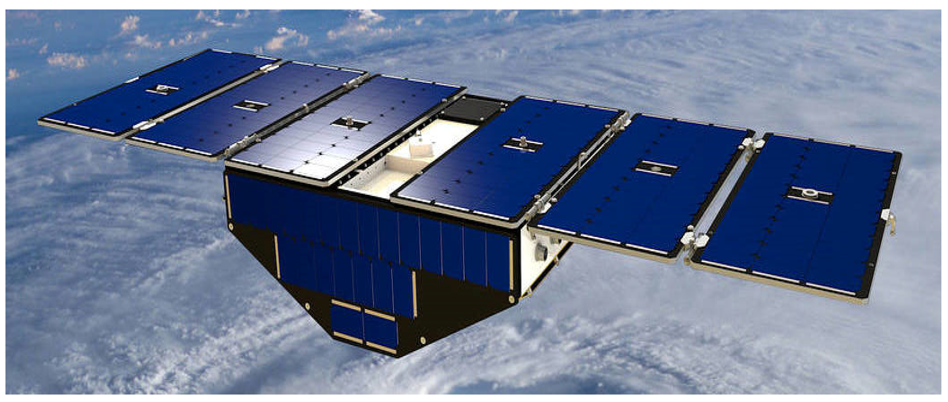
Attitude determination and control is a critical subsystem on the majority of modern spacecraft like that depicted in Figure 1. Rotational dynamics and kinematics, actuators, sensors and observers, controllers, and perturbations are all expansive areas of research into ensuring the desired pointing and spin of a given craft is achieved. Traditional linearized feedback control is anything but simple and robust. Extensive analysis of poles, gain design, and analysis on the boundaries of where linearization still holds true all pose consistent challenges even in simple implementations of traditional proportional-integral-derivative (PID). Large amounts of thought are put into designing controllers for their specific implementations and their performances are highly restricted to the anticipated environment for which they were designed. To address the limitations of linearization, non-linear feedforward techniques were developed. Though more robust than traditional feedback (and in theory capable of exact control), feedforward control also has innate restrictions. It requires highly accurate process modeling that is easily disturbed by unaccounted for noise. deterministic artificial intelligence conveniently ignores environmental noise and requires only knowledge of rotational dynamics. By assuming the physics will hold true (which it always will), we can create highly accurate and robust controllers. In conjunction with feedback and feedforward control, our new hybrid control can perform accurately in a wide range of environments and shifting variables.
Attitude control of space vehicles is complicated by external forces and torques and unfortunately sometimes collision damage due to coincident orbital events. Significant research in the topic follows several lines seeking to negate such complicating factors. A long list of techniques in the lineage include classical feedback, feedforward (more relatively rare), optimal control, robust control (typically a label for optimal control minimizing the infinity norm of specified cost function), and several nonlinear adaptive techniques like self-tuning regulators and model-reference adaptive control. Another recent technique is physics-based control. Several of these techniques necessitate autonomous formulation of attitude trajectories and several options predominate. Especially noting the utilization of the eigenaxis [3] by the four-dimensional parameterization of three-dimensional rotation (the “quaternion”), so-called eigen-axis maneuvers [4] utilize the eigen-axis to define the shortest-distance between two point (the initial point and the desired point). Subsequent demonstration that shortest distance does not lead to minimum time maneuvers, [5] alternative options for autonomous trajectory generation abound. Having the control follow a “sliding-mode” manifold [6,7] defined as by linearity with a nonlinear control forcing the trajectory to follow the sliding mode, where Zou et al., [8] also sought to introduce learning using a stochastic (non-deterministic) neural network. Wang et al., [9] sought to include actuator dynamics while Wang et al., [10] incorporated vehicle structural flexibility.
Nonlinear adaptive techniques established the provenance of self-awareness statements in deterministic artificial intelligence (later combined with physics-based controls). Slotine proposed nonlinear adaptive methods for robotics [11] with parallel development for spacecraft attitude control [12] culminating in the finalized development of both presented as advanced material in the textbook Applied Nonlinear Control. [13] The method essentially utilized classic feedback to adapt a feedforward and feedback signals in addition to adaptive the trajectory fed to both feedforward and feedback channels. The foundational work parameterized the control in the non-rotating, non-accelerating inertial reference frame, while Fossen [14] proposed improved performance (computational efficiency) with analytically identical control formulated in the rotating body reference frame. Fossen illustrated broad, general applicability to underwater robotics and underwater vehicles in general [15,16], and this generalization continued eventually culminating in similar demonstrations for the currently instantiation of deterministic artificial intelligence.
After Fossen’s evolutions, the feedforward and feedback gains were proven to be separately tunable [17,18], while the former works combined tuning of both. The evolving techniques were augmented by physics-based control methods of Lorenz [19] formerly applied to torque control [20] but also applied specifically to deadbeat torque generation, induction machines [21], multi-phase electric motors [22], magnetic state control [23], loss-minimizing servo control [24], magnetic flux control [25], self-sensing control [26], and brushed DC motor control [27] eventually illustrating efficacy for spacecraft attitude control [28] as an augmentation to the lineage of methods started by Slotine.
Regarding the feedforward channel, the most recent developments proposed methods for dealing with highly nonlinear oscillatory van der Pol circuits [29] necessitating state observers [30] to permit applicability in feedback [31] as learning by Smeresky and Rizzo to spacecraft attitude control. Following this success, very similarly to the earlier lineage, the methods were applied to unmanned underwater vehicles [32] and DC motor control [33] where an interesting comparison to foundational nonlinear adaptive control was offered by Shah [34]. So far, this year the current instantiation of deterministic artificial intelligence has been applied to remote underwater vehicles by Osler [35], while the necessary autonomous trajectory generation schemes currently in use were critically compared by Sandberg [36] following Koo’s elaboration [37] of the impacts on trajectories of discretization and numerical propagation. Sandberg’s trajectory generation results were enhanced by Raigoza [38] to include satellite de-orbiting with autonomous obstacle avoidance.
This considerable background literature display gaps emphasized strongly by the instantiation of the work presented here, and based on the major gaps of overcoming uncertainties, the claimed contributions of the article are justified. One major feature offered by the self-awareness statements of deterministic artificial intelligence obfuscates the necessity in the stochastic approaches to categorize uncertainties as internal or external, parametric or non-parametric, constant, characteristic or random. In real time applications the physical, mechanical, electrical and environmental constraints are addressable in real time environments by a priori utilization of real-time optimization techniques presented by Sandberg in [36].
Artificial intelligence is ubiquitously described as intrinsically stochastic, implying machine learning, most often utilizing neural networks and often augmented with deep learning. While this manuscript utilizes a number of uncertainties, disturbances and noises the algorithm remains deterministic in the assertion of self-awareness (offered by Cooper and Heidlauf’s methodology), relegating the stochastic forms of artificial intelligence to counteract the unknowable features.
Smeresky and Rizzo [31] showed that deterministic artificial intelligence could achieve improved results compared to both optimized feedback and feedforward control schemes. Additionally, it achieved reduced computational burden. Building off their work, this manuscript presents a redesigned deterministic artificial intelligence controller in conjunction with Smeresky’s optimal feedback and feedforward control and evaluates the proposed method to overcome a range of environmental disturbances (not formerly in the literature) including a sudden shift in the values of the craft’s mass moments of inertia, while the controller was tuned with no such knowledge. Despite this sudden shift and range of disturbances, the controller exceeded expectations and demonstrated consistent stability. Mean trajectory tracking error was improved over 91%, while the standard deviation was improved over 97% whilst improving (reducing) control effort by 13%.
2. Materials and Methods
Comparisons of the various algorithms should be performed under equal conditions. Therefore, the validating simulations displayed in Appendix A illustrate identical conditions where algorithms are switched on when active, while others are deactivated. The parameters of the respective algorithms are chosen seeking identical final values when initiated from identical initial conditions.
2.1. Rigid Body Motion
The topic of rigid body motion is best described in a Euler’s Equation for rigid body motion displayed in Equation (1) (reference Table 1 for variable definitions in Equation (1)).
This is the rotational equivalent of newton’s second law relating the acceleration of an object to the fore applied to it. It is the basis of action from the controllers and actuators on the craft, determining the exact quantity of torque necessary to shift the angular momentum of the craft to a specific direction and magnitude.
2.2. PDI Control
Traditional PID control functions around a linearized control point as illustrated in Equation (2) (reference Table 2 for variable definitions in Equations (2) and (3)).
We implement a non-linear enhanced control called proportional-integral-derivative (PDI) of the form displayed in Equation (3).
This controller accounts for both position and velocity errors, better reflecting the true physics of the non-linear system we are modeling. Additionally, it contains a non-linear decoupling term ( to account for the constantly shifting reference frames.
2.3. Luenberger Observers
We implement an observer of the form displayed in Equation (4) (reference Table 3 for variable definitions in Equation (4)).
where (k) is the kth estimated state vector, (k) is the kth estimated output vector. Ad is the discretized state matrix, is the discretized input matrix, and is the observer gain matrix.
2.4. Deterministic Artificial Intelligence (DAI)
While feedback (PDI) and feedforward control have proven applications and functionality, they both suffer flaws. Feedback (PDI) control contains no analytical solution, as one is equating a derivative and integral to an exact physical value, hence the consistent error and oscillation in steady state of all feedback (PDI) solutions. Adaptive Feedforward control could in theory provide exact solutions, but only with perfect knowledge of all system and environmental parameters, again impossible. deterministic artificial intelligence seeks to provide an exact analytical solution without knowledge of environmental parameters, by enforcing new assumptions on your physical system, a system who’s physics one can characterize exactly. In this case, we focus purely on three degree of freedom rotational control according to Euler’s equations for rotational rigid body motion. Our estimable system parameter of inertia will allow us to enforce desirable physics on our control algorithm via the self-awareness statement displayed in Equation (5) (reference Table 4 for variable definitions in Equations (5)–(7)). whose system matrix is displayed in Equation (6) and regression vector in Equation (7). Equation (6) in particular illustrates the novel method of insuring trajectory tracking, where the control definition embeds the coupled, nonlinear desired trajectory annotated by the subscript, d. As estimates converge to actual values, trajectory tracking is assured by actual states converging to desired states.
where:
And
Incorporating this knowledge with our observer output, we can estimate a (the difference in our desired state inertia vs. our current state inertia) via the Moore-Penrose pseudo inverse (the 2-norm optimal solution to our self-awareness statement). This gives an output control that enforces our system inertia to match its actual behavior, thus producing a more robust response regardless of any present disturbances.
Using our learned , we can enforce an additional control input proportional to in addition that of our PID algorithm. While the DAI control can exist on its own, in this paper we only cover the pure PID and hybrid PID/DAI cases.
Existing machine learning techniques in vehicle control attempt to match assumptions about highly non-linear real-world equations of motion and matching control outputs based on environmental experience. Inherently, these methods will be non-robust as the introduction of novel inputs to their schemas will produce undesirable results until the algorithm readapts. For example, if a reinforcement learning model is trained to control an aerial vehicle in laminar flow conditions, the introduction of turbulent conditions will introduce unknown equations of motion that will threaten stability. DAI, in contrast, assumes any estimated control input to produce a desired change in motion is inherently false (as we do not have perfect knowledge of the multitude of effects that can change vehicle dynamics). To counter this problem, it simplifies the error to a change in vehicle parameters (parameters that we know will affect the equations of motion we are seeking to modify, in this case inertia). The “learning” is instantaneous and not necessarily reflective of the true state of the vehicle, but it is reflective of the effective state in the face of unknown perturbations.
3. Results
This section will compare combined feedforward and feedback control (FFD + FB) to combined feedforward and feedback control with deterministic artificial intelligence (FFD + FB + DAI). First, we will compare performances of the schemes for a thirty-degree yaw with no disturbances. Next, we will perform the same maneuver with simulated gravitational gradient and drag torques to evaluate the efficacy of each approach to handle the disturbance inputs without their explicit presence in the respective approach. Lastly, we simulate a large one-hundred-degree yaw with perturbations and a change in the craft’s dynamics via a sudden shift in inertia. Visualization, initialization, and data processing code are provided in Appendix B. The exact values for simulation startup and input parameters are provided in Appendix C. Observer and controller gains are listed in Table 5.
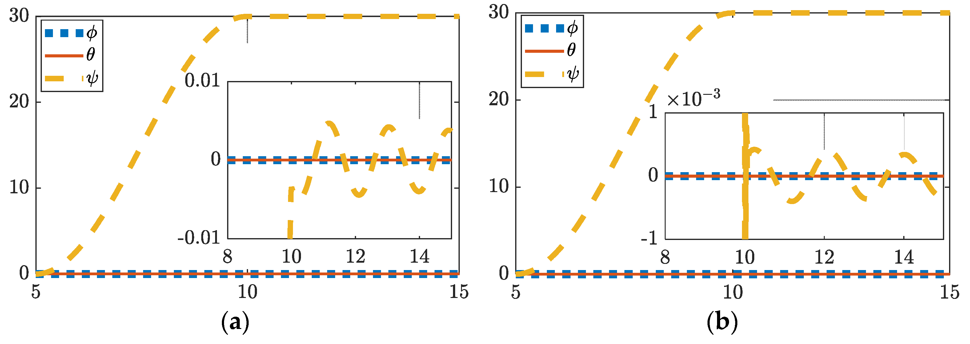
3.1. Thirty-Degree Yaw
The plots in Figure 2 show that just over one order of magnitude of precision is gained via deterministic artificial intelligence implementation. Exact values of improvement are listed in Table 6. While traditional control settles to degrees of error, deterministic artificial intelligence hybrid control settles to degrees of error in a fraction of the amount of time. Additionally, deterministic artificial intelligence runs in 18.2 s while traditional optimal control takes 21.3 s, showing both a boost in speed and accuracy.
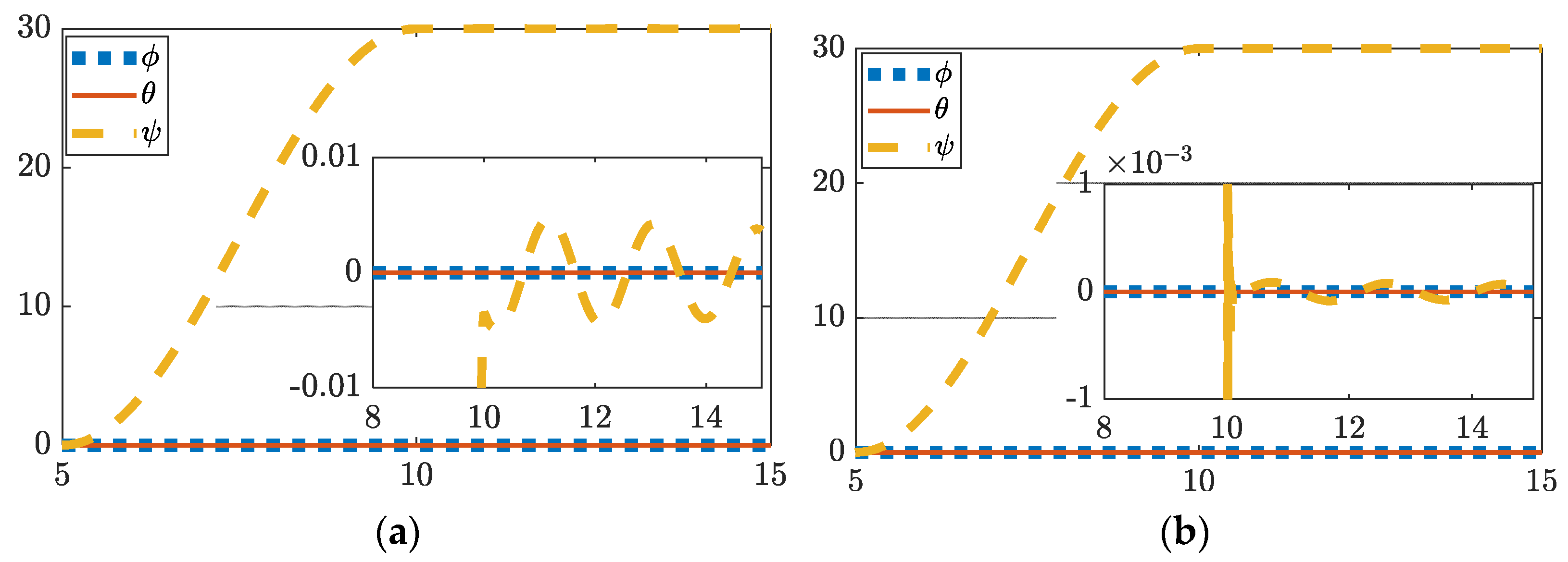
3.2. 30 Degree Yaw with Perturbations
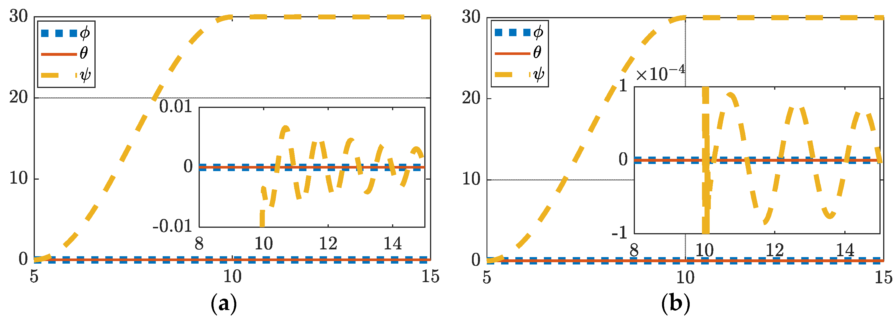
3.3. One-Hundred-Degree Yaw Maneuver with Perturbations and Simulated Damage
4. Discussion
While it was anticipated that the hybrid deterministic artificial intelligence approach would yield optimal results per the work of Smeresky and Rizzo, one surprising outcome was the reduction of error in the presence of persistent excitation. Any level of observer noise improved the precision of the deterministic artificial intelligence controller. In simulation, this can be difficult to model but a real-world implementation of deterministic artificial intelligence would yield continuous noise inputs from sensors and thus more accurate controls.
Both controllers seemed to handle sudden changes in spacecraft inertia (and thus its dynamics), quite well, with minimal effect on the actual control. As displayed in Table 9, mean trajectory tracking error was improved over 91%, while the standard deviation was improved over 97% whilst improving (reducing) control effort by 13%. It should be noted that the observer proportional-derivative-integral (PDI) gains were set quite aggressively and may not be feasible for real life actuators to implement. Further work should be done to explore deterministic artificial intelligence with control signals restricted by the capabilities of real-world actuators.
One final further route to explore would be to implement the output of the deterministic artificial intelligence controller to update the controller side inertia estimate. This may allow for faster control in the face of damage, along with being a useful diagnostic tool for remote vehicles.
Author Contributions
Conceptualization, T.S.; Formal analysis, E.W.; Funding acquisition, T.S.; Investigation, E.W.; Methodology, T.S.; Project administration, T.S.; Resources, T.S.; Software, E.W.; Supervision, T.S.; Validation, E.W. and T.S.; Visualization, E.W.; Writing—original draft, E.W.; Writing—review & editing, E.W. and T.S. All authors have read and agreed to the published version of the manuscript.
Funding
This research received no external funding.
Institutional Review Board Statement
Not applicable.
Informed Consent Statement
Not applicable.
Data Availability Statement
Data is available by contacting the corresponding author.
Acknowledgments
The authors thank Cornell University and the U.S. Naval Postgraduate School for continued support of graduate research and learning.
Conflicts of Interest
The authors declare no conflict of interest. Authors have no personal circumstances or interest that may be perceived as inappropriately influencing the representation or interpretation of reported research results.
Appendix A
Appendix A contains topologies and software crucial to understanding and reproducing the research shown.
Appendix A.1. Simulink Model
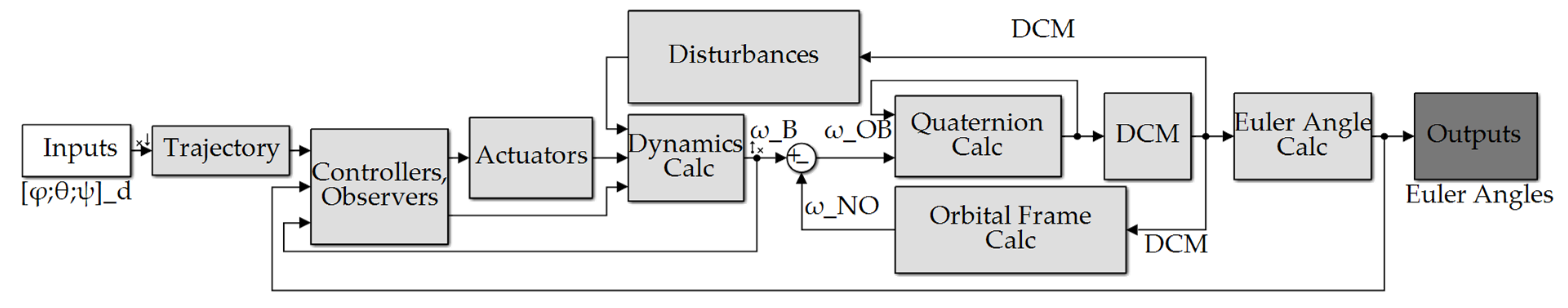
Figure A1.
Simulink model overview.

Figure A2.
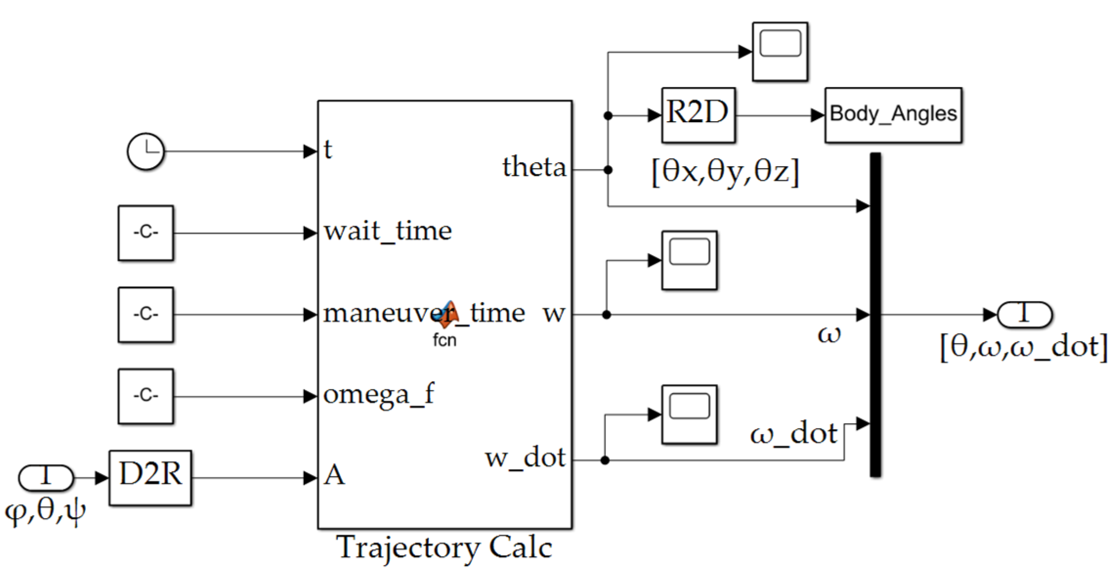
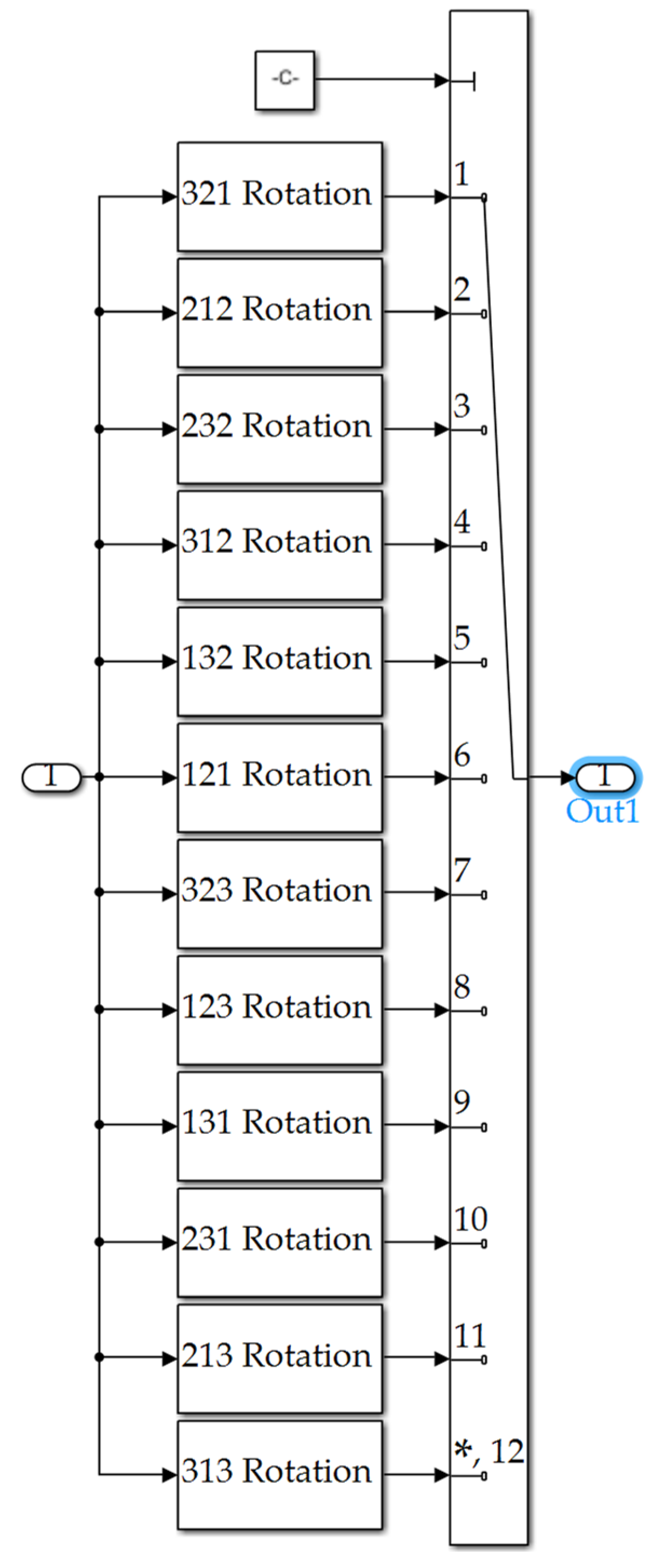
Trajectory subsystem depicted in Figure A1.
Figure A2.
Trajectory subsystem depicted in Figure A1.

Figure A3.
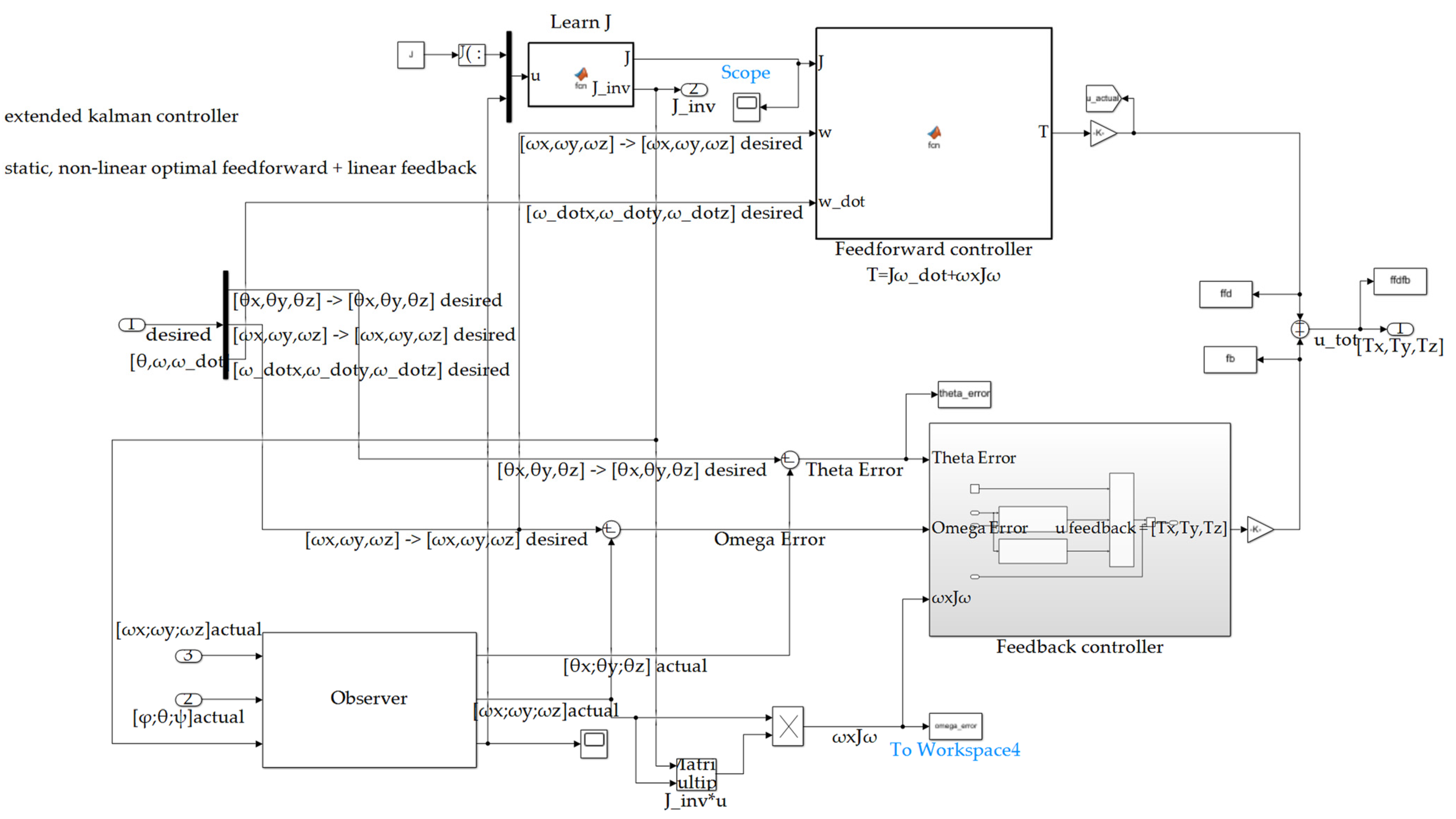
controllers’ and observers’ subsystem depicted in Figure A1.
Figure A3.
controllers’ and observers’ subsystem depicted in Figure A1.

Appendix A.2. Learn [J] Subsystem Function File Depicted in Figure A3
function [J,J_inv] = fcn(u)
%At T = 8, simulate damage
% if u(16) == 8
% u(1) = 0.7*u(1); u(5) = 0.3*u(5); u(9) = 0.65*u(9);
% end
J = zeros(3,3);
J(1,1) = u(1) + u(10); J(1,2) = u(2) + u(11); J(1,3) = u(3) + u(12);
J(2,1) = u(4) + u(11); J(2,2) = u(5) + u(13); J(2,3) = u(6) + u(14);
J(3,1) = u(7) + u(12); J(3,2) = u(8) + u(14); J(3,3) = u(9) + u(15);
% J = [J(1) J(2) J(3); J(4) J(5) J(6); J(7) J(8) J(9)];
J_inv = J\eye(length(J)); %J_inv = inv(J); %J_inv = eye(3,3)\J;
%set_param(‘AE3818_HW6_v3_simulink/J’,’Value’,[J(1:3);J(4:6);J(7:9)]);
Appendix A.3. Feedforward Control Subsystem Function File Depicted in Figure A3
function T = fcn(J,w,w_dot)
%Unpack the input data
Jxx = J(1); Jxy = J(2); Jxz = J(3);
Jyx = J(4); Jyy = J(5); Jyz = J(6);
Jzx = J(7); Jzy = J(8); Jzz = J(9);
wx = w(1); wy = w(2); wz = w(3);
wx_dot = w_dot(1); wy_dot = w_dot(2); wz_dot = w_dot(3);
%Calculate the torques
Tx = Jxx*wx_dot+Jxy*wy_dot+Jxz*wz_dot-Jxy*wx*wz-Jyy*wy*wz-Jyz*wz^2+Jxz*wx*wy+Jzz*wz*wy+Jyz*wy^2;
Ty = Jyx*wx_dot+Jyy*wy_dot+Jyz*wz_dot-Jyz*wx*wy-Jzz*wx*wz-Jxz*wx^2+Jxx*wx*wz+Jxy*wz*wy+Jxz*wz^2;
Tz = Jzx*wx_dot+Jzy*wy_dot+Jzz*wz_dot-Jxx*wx*wy-Jxz*wy*wz-Jxy*wy^2+Jyy*wx*wy+Jyz*wz*wx+Jxy*wx^2;
%Package the output
T = [Tx;Ty;Tz];
end
Figure A4.
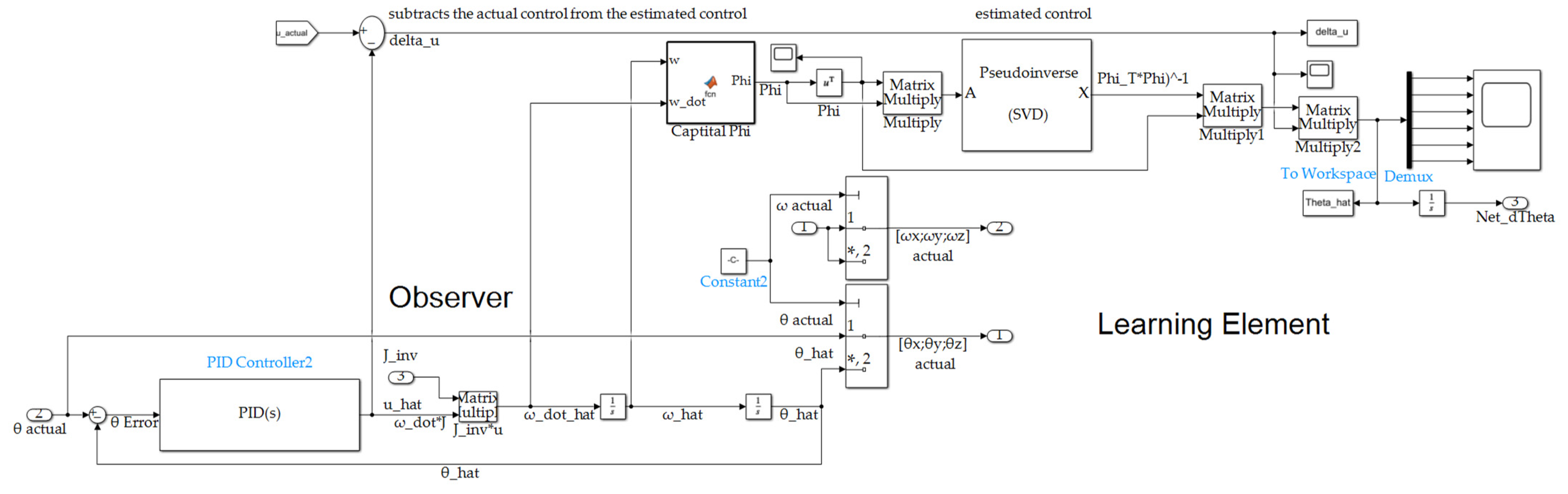
Observer subsystem depicted in Figure A3.
Figure A4.
Observer subsystem depicted in Figure A3.

Figure A5.
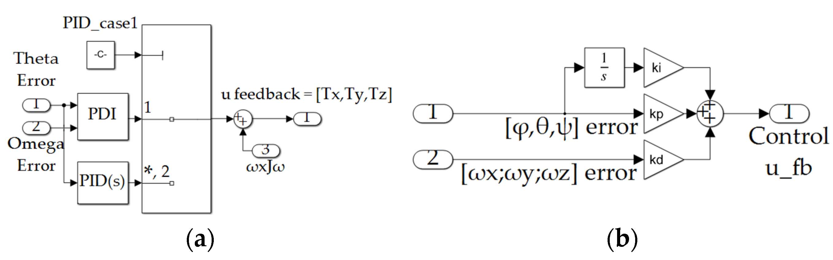
(a) Feedback controller subsystem depicted in Figure A3; (b) proportional, derivative, integral controller depicted in subfigure (a).
Figure A5.
(a) Feedback controller subsystem depicted in Figure A3; (b) proportional, derivative, integral controller depicted in subfigure (a).

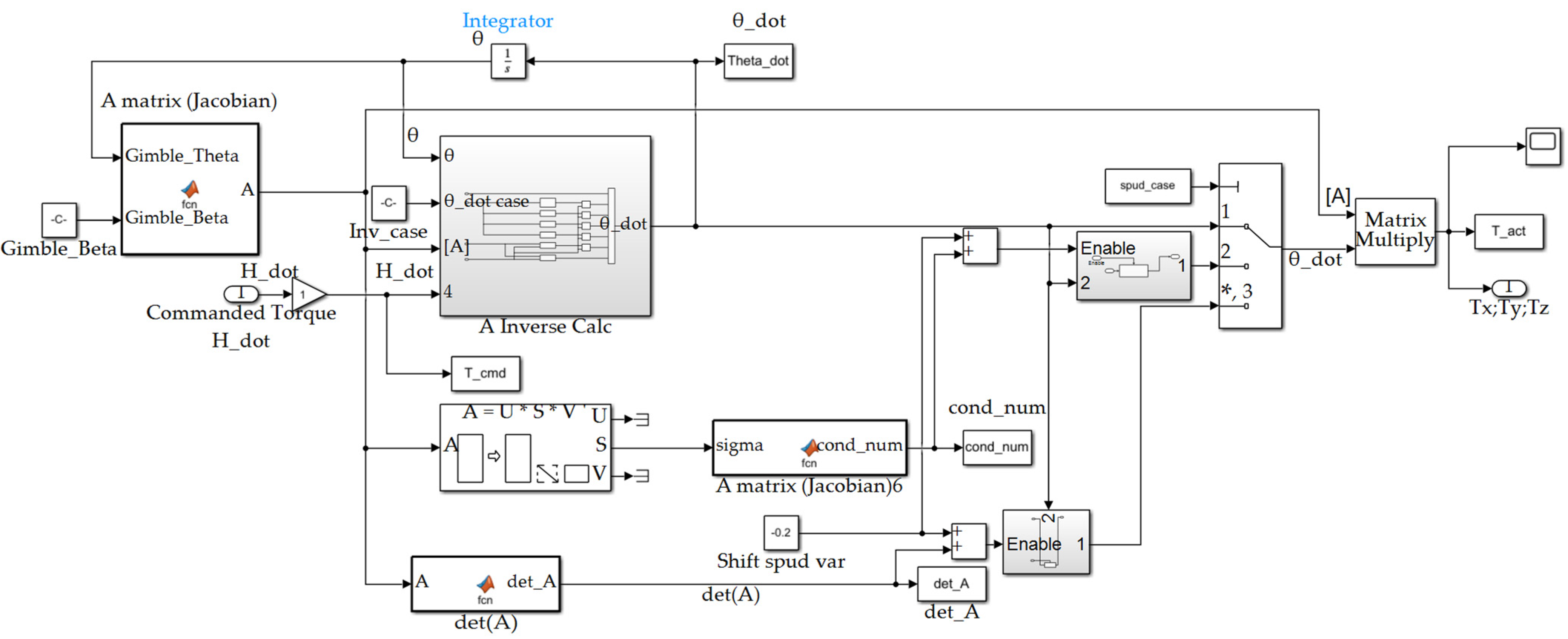
Figure A6.
Actuators’ subsystem depicted in Figure A1.
Figure A6.
Actuators’ subsystem depicted in Figure A1.

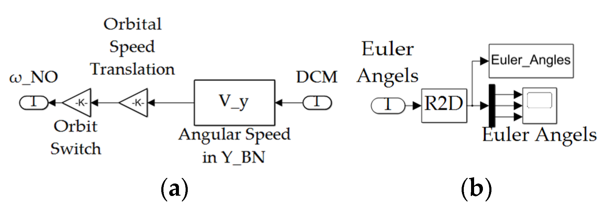
Figure A7.
(a) Orbital frame calc subsystem depicted in Figure A1; (b) Euler angles output subsystem depicted in Figure A1.

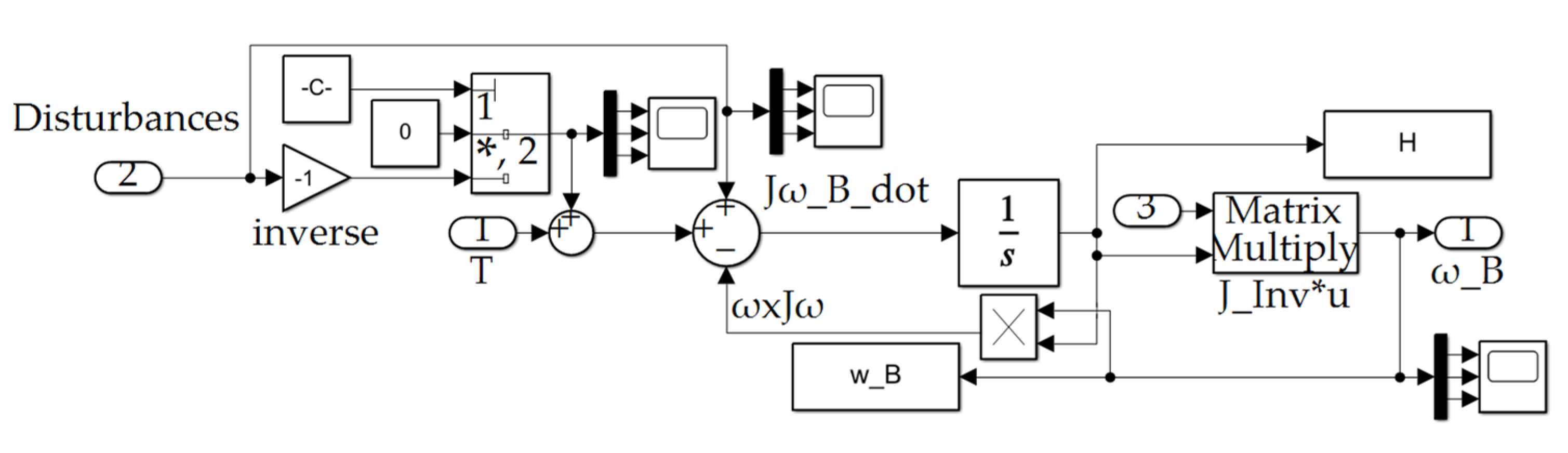
Figure A8.
Dynamics Calc subsystem depicted in Figure A1.
Figure A8.
Dynamics Calc subsystem depicted in Figure A1.

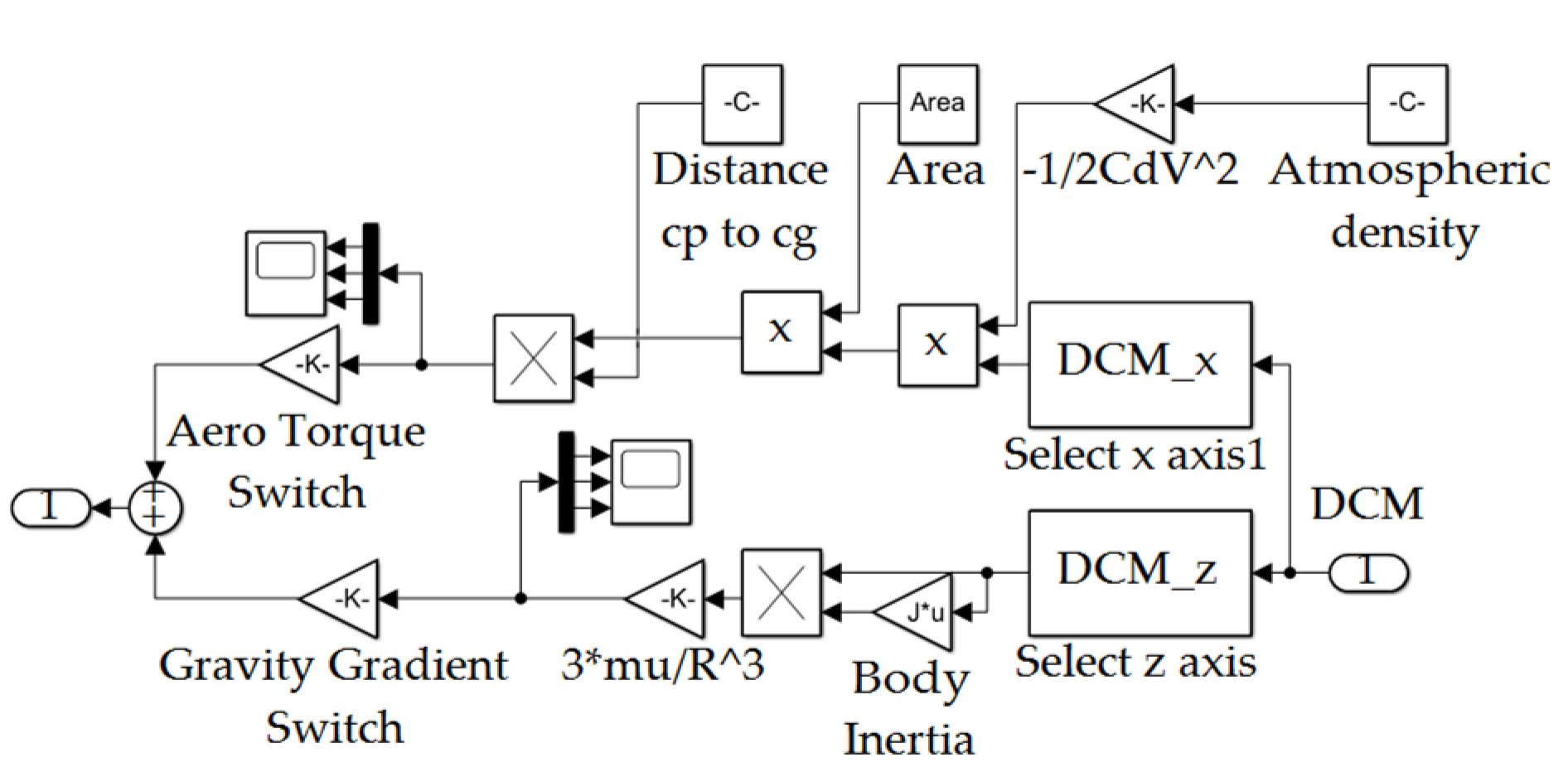
Figure A9.
Disturbances’ subsystem depicted in Figure A1.
Figure A9.
Disturbances’ subsystem depicted in Figure A1.

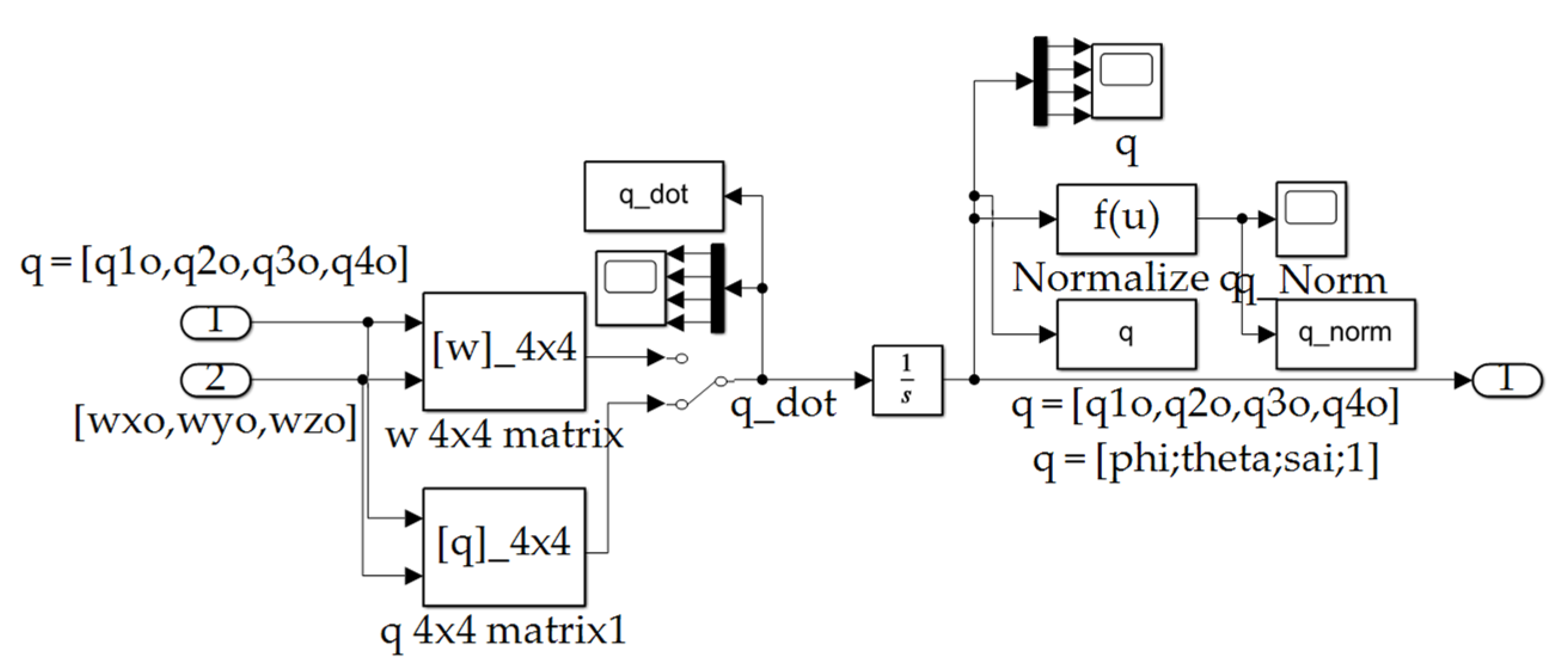
Figure A10.
Quaternion Calc subsystem depicted in Figure A1.
Figure A10.
Quaternion Calc subsystem depicted in Figure A1.

Appendix A.4. [ω]_([4 × 4])Subsystem Depicted in Figure A10 Constructing Direction Cosine Matrix from Angular Velocity
function q_dot = fcn(q,w)
q = [q(1);q(2);q(3);q(4)];
w_matrix = 1/2*…
[ 0, w(3), -w(2), w(1);…
-w(3), 0, w(1), w(2);…
w(2), -w(1), 0, w(3);…
-w(1), -w(2), -w(3), 0];
q_dot = w_matrix*q;
Appendix A.5. [q]_([4 × 4]) Subsystem Depicted in Figure A10 Constructing Direction Cosine Matrix from Quaternion Vector
function q_dot = fcn(q,w)
w = [w(1);w(2);w(3);0];
q_matrix = 1/2*…
[q(4), -q(3), q(2), q(1);…
q(3), q(4), -q(1), q(2);…
-q(2), q(1), q(4), q(3);…
-q(1), -q(2), -q(3), q(4)];
q_dot = q_matrix*w;
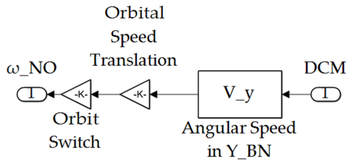
Figure A11.
Orbital Frame Calc subsystem depicted in Figure A1.
Figure A11.
Orbital Frame Calc subsystem depicted in Figure A1.

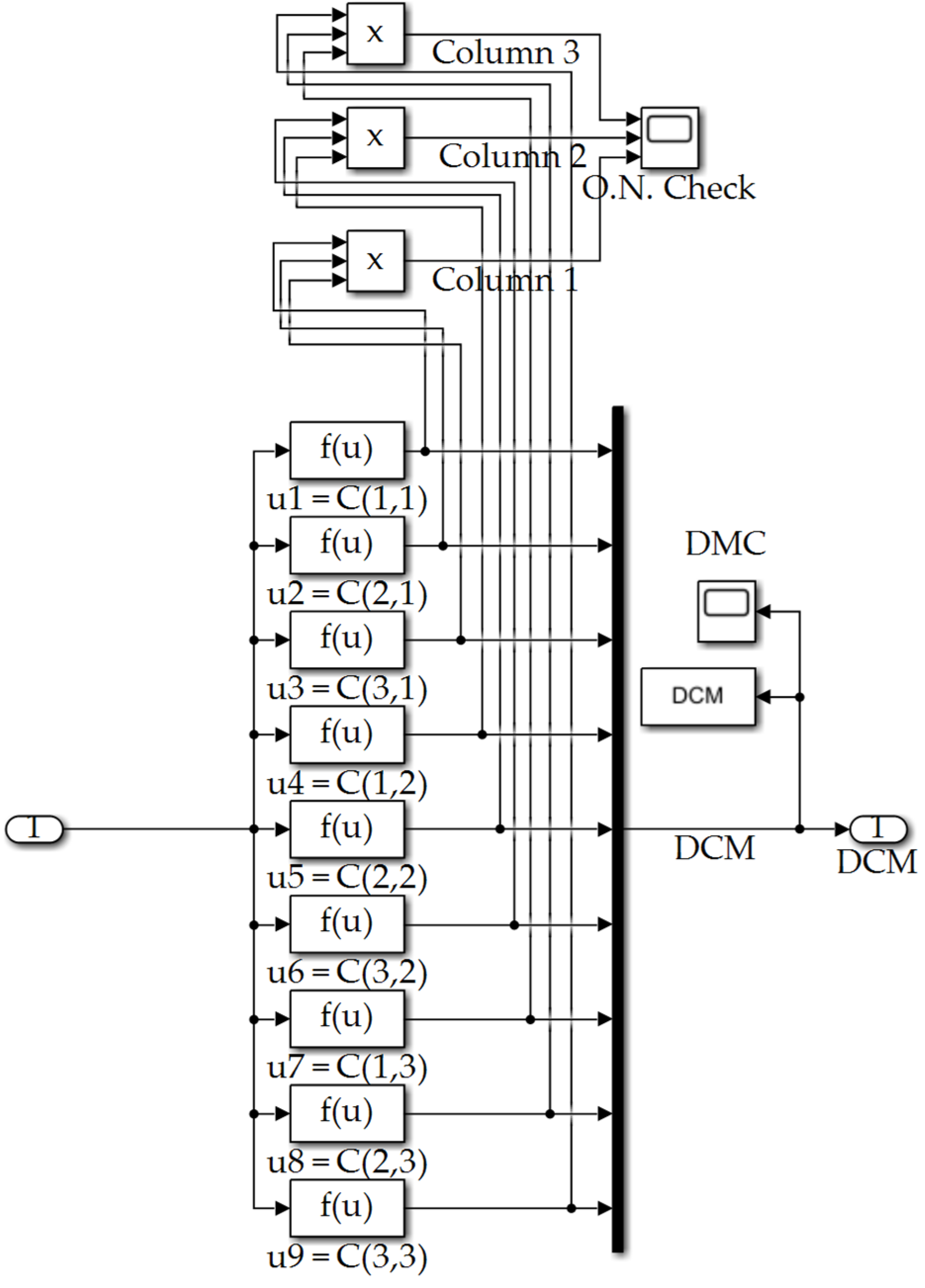
Figure A12.
DCM subsystem depicted in Figure A1.
Figure A12.
DCM subsystem depicted in Figure A1.

Figure A13.
Euler Angle Calc subsystem depicted in Figure A1.
Figure A13.
Euler Angle Calc subsystem depicted in Figure A1.

Appendix B. Wrapper MATLAB Line Code
% Clear all variables, figures, and outputs
clear all; clc; close all;
% GLOBAL VARIABLE DECLARATIONS/////////////////////////
% This section is where global variables are defined
% NONE
% END GLOBAL VARIABLES\\\\\\\\\\\\\\\\\\\\\\\\\
% FORMATTING BEHAVIOR/////////////////////////
% This section is where formatting behavior is defined
setgraphics()
% END FORMATTING BEHAVIOR\\\\\\\\\\\\\\\\\\\\\\\\\
% MAIN/////////////////////////
% This section is main function
disp ‘Main -------------------------’;
% J = [50.5 0.1 0.1; 0.1 75.2 0.1; 0.1 0.1 one-hundred.4];
% %J = [2.0 0.1 0.1; 0.1 2.0 0.1; 0.1 0.1 2.0]; %For an uglier J
% J_Inv = J\eye(length(J));
%Load Simulink files
load_system(‘AE3818_HW6_v3_simulink.slx’);
model = ‘AE3818_HW6_v3_simulink’;
%Run Simulink models:
%Set the input parameters
wait_time = 5; % Seconds
maneuver_time = 20; % Seconds
post_maneuver_time = thirty; % Seconds
orbital_Gain_Switch = 0; % 0 = Orbital disturbances off, 1 = on
aero_torque_Switch = 0; % 0 = aero torque disturbances off, 1 = on
gravity_gradient_Switch = 0; % 0 = gravity disturbances off, 1 = on
dist_correct_switch = 1; %1 = off, 2 = on
Rotation_Var = 1; %Select the DCM to Euler Angle Rotation scheme
Inv_case = 1; % Inverse calculated via pseudoinv
spud_case = 1; % 1 = SPUD off, 0 = SPUD on
case_Var = [0,0,thirty]; %The commanded Euler Angle
PID_case = 1; % Feedback controller method 1 = proportional, derivative, integral, 2 = Matlab PID
kp = one-hundred0; % Kp gain for controller
kd = 10; % Kd gain for controller
ki = 0.1; % Ki gain for controller
observer_case = 2; % 1 = observer off, 2 = observer on
kp2 = one-hundred000; % Kp gain for controller
kd2 = 500; % Kd gain for controller
ki2 = 0.1; % Ki gain for controller
% I. Scenario cases
% A. Case 1—large timestep ffd+fb
disp(‘Case 1’)
timestep = 0.01; %Seconds
set_param(model,’FixedStep’,num2str(timestep),’StopTime’,…
num2str(wait_time+maneuver_time+post_maneuver_time));
ffd_case = 1; % 1 = ffd control on, 0 = ffd control off
fb_case = 1; % 1 = fb control on, 0 = fb control off
tic;
[case1.time,~,~] = sim(model);
case1.runtime = toc; %Get timing data
%Retrieve data from Simulink
case1.q_dot = q_dot;
case1.q = q;
case1.q_norm = q_norm;
case1.DMC = DCM;
case1.H = H;
case1.w_B = w_B;
case1.Euler_Angles = Euler_Angles;
case1.Body_Angles = Body_Angles;
case1.T_cmd = T_cmd;
case1.T_act = T_act;
case1.Theta_dot = Theta_dot;
case1.cond_num = cond_num;
case1.detA = det_A;
case1.ffd = ffd;
case1.fb = fb;
case1.ffdfb = ffdfb;
case1.theta_error = theta_error;
case1.omega_error = omega_error;
case1.delta_u = delta_u;
case1.Theta_hat = Theta_hat;
% B. Case 2—small timestep ffd+fb
disp(‘Case 2’)
timestep = 0.001; %Seconds
set_param(model,’FixedStep’,num2str(timestep),’StopTime’,…
num2str(wait_time+maneuver_time+post_maneuver_time));
ffd_case = 1; % 1 = ffd control on, 0 = ffd control off
fb_case = 1; % 1 = fb control on, 0 = fb control off
tic;
[case2.time,~,~] = sim(model);
case2.runtime = toc; %Get timing data
%Retrieve data from Simulink
case2.q_dot = q_dot;
case2.q = q;
case2.q_norm = q_norm;
case2.DMC = DCM;
case2.H = H;
case2.w_B = w_B;
case2.Euler_Angles = Euler_Angles;
case2.Body_Angles = Body_Angles;
case2.T_cmd = T_cmd;
case2.T_act = T_act;
case2.Theta_dot = Theta_dot;
case2.cond_num = cond_num;
case2.detA = det_A;
case2.ffd = ffd;
case2.fb = fb;
case2.ffdfb = ffdfb;
case2.theta_error = theta_error;
case2.omega_error = omega_error;
case2.delta_u = delta_u;
case2.Theta_hat = Theta_hat;
% C. Case 3—large timestep, ffd on, fb off
disp(‘Case 3’)
timestep = 0.001; %Seconds
set_param(model,’FixedStep’,num2str(timestep),’StopTime’,…
num2str(wait_time+maneuver_time+post_maneuver_time));
ffd_case = 1; % 1 = ffd control on, 0 = ffd control off
fb_case = 0; % 1 = fb control on, 0 = fb control off
tic;
[case3.time,~,~] = sim(model);
case3.runtime = toc; %Get timing data
%Retrieve data from Simulink
case3.q_dot = q_dot;
case3.q = q;
case3.q_norm = q_norm;
case3.DMC = DCM;
case3.H = H;
case3.w_B = w_B;
case3.Euler_Angles = Euler_Angles;
case3.Body_Angles = Body_Angles;
case3.T_cmd = T_cmd;
case3.T_act = T_act;
case3.Theta_dot = Theta_dot;
case3.cond_num = cond_num;
case3.detA = det_A;
case3.ffd = ffd;
case3.fb = fb;
case3.ffdfb = ffdfb;
case3.theta_error = theta_error;
case3.omega_error = omega_error;
case3.delta_u = delta_u;
case3.Theta_hat = Theta_hat;
% D. Case 4—large timestep, ffd off, fb on
disp(‘Case 3’)
timestep = 0.001; %Seconds
set_param(model,’FixedStep’,num2str(timestep),’StopTime’,…
num2str(wait_time+maneuver_time+post_maneuver_time));
ffd_case = 0; % 1 = ffd control on, 0 = ffd control off
fb_case = 1; % 1 = fb control on, 0 = fb control off
tic;
[case4.time,~,~] = sim(model);
case4.runtime = toc; %Get timing data
%Retrieve data from Simulink
case4.q_dot = q_dot;
case4.q = q;
case4.q_norm = q_norm;
case4.DMC = DCM;
case4.H = H;
case4.w_B = w_B;
case4.Euler_Angles = Euler_Angles;
case4.Body_Angles = Body_Angles;
case4.T_cmd = T_cmd;
case4.T_act = T_act;
case4.Theta_dot = Theta_dot;
case4.cond_num = cond_num;
case4.detA = det_A;
case4.ffd = ffd;
case4.fb = fb;
case4.ffdfb = ffdfb;
case4.theta_error = theta_error;
case4.omega_error = omega_error;
case4.delta_u = delta_u;
case4.Theta_hat = Theta_hat;
% II. Analysis and Plots
% Timestep analysis plots
figure(1);
subplot(1,3,1);
plot(case1.time, case1.Euler_Angles(:,1),’-’,…
case2.time, case2.Euler_Angles(:,1),’:’);
title(‘$\phi$ Time-step Analysis ffd+fb’);
legend(‘0.01 Time-step’,’0.001 Time-step’,’location’,’best’)
subplot(1,3,2);
plot(case1.time, case1.Euler_Angles(:,2),’-’,…
case2.time, case2.Euler_Angles(:,2),’:’);
title(‘$\theta$ Time-step Analysis ffd+fb’);
legend(‘0.01 Time-step’,’0.001 Time-step’,’location’,’best’)
subplot(1,3,3);
plot(case1.time, case1.Euler_Angles(:,3),’-’,…
case2.time, case2.Euler_Angles(:,3),’:’);
title(‘$\psi$ Time-step Analysis ffd+fb’);
legend(‘0.01 Time-step’,’0.001 Time-step’,’location’,’best’)
figure(20);
subplot(2,3,1);
plot(case1.time, case1.theta_error(:,1),’-’,…
case2.time, case2.theta_error(:,1),’:’);
title(‘$\theta_x$ error to feedback controller’);
legend(‘0.01 Time-step’,’0.001 Time-step’,’location’,’best’)
subplot(2,3,2);
plot(case1.time, case1.theta_error(:,2),’-’,…
case2.time, case2.theta_error(:,2),’:’);
title(‘$\theta_y$ error to feedback controller’);
legend(‘0.01 Time-step’,’0.001 Time-step’,’location’,’best’)
subplot(2,3,3);
plot(case1.time, case1.theta_error(:,3),’-’,…
case2.time, case2.theta_error(:,3),’:’);
title(‘$\theta_z$ error to feedback controller’);
legend(‘0.01 Time-step’,’0.001 Time-step’,’location’,’best’)
subplot(2,3,4);
plot(case1.time, case1.omega_error(:,1),’-’,…
case2.time, case2.omega_error(:,1),’:’);
title(‘$\omega_x$ error to feedback controller’);
legend(‘0.01 Time-step’,’0.001 Time-step’,’location’,’best’)
subplot(2,3,5);
plot(case1.time, case1.omega_error(:,2),’-’,…
case2.time, case2.omega_error(:,2),’:’);
title(‘$\omega_y$ error to feedback controller’);
legend(‘0.01 Time-step’,’0.001 Time-step’,’location’,’best’)
subplot(2,3,6);
plot(case1.time, case1.omega_error(:,3),’-’,…
case2.time, case2.omega_error(:,3),’:’);
title(‘$\omega_z$ error to feedback controller’);
legend(‘0.01 Time-step’,’0.001 Time-step’,’location’,’best’)
% Show ffd,fb,ffd+fb control inputs on a 1x3 plot
figure(2);
subplot(1,3,1);
plot(case2.time, case2.ffd(:,1),…
case2.time, case2.ffd(:,2),…
case2.time, case2.ffd(:,3));
title(‘feedforward control’);
legend(‘$\phi$’,’$\theta$’,’$\psi$’,’location’,’best’)
subplot(1,3,2);
plot(case2.time, case2.fb(:,1),…
case2.time, case2.fb(:,2),…
case2.time, case2.fb(:,3));
title(‘feedback control’);
legend(‘$\phi$’,’$\theta$’,’$\psi$’,’location’,’best’)
subplot(1,3,3);
plot(case2.time, case2.ffdfb(:,1),…
case2.time, case2.ffdfb(:,2),…
case2.time, case2.ffdfb(:,3));
title(‘feedforward plus feedback control’);
legend(‘$\phi$’,’$\theta$’,’$\psi$’,’location’,’best’)
% Show ffd vs fb euler angle analysis
% case3 = ffd only, case4 = fb only, case 1 = ffd+fb
figure(3);
subplot(2,3,1);
plot(case3.time, case3.Euler_Angles(:,1),’:’,…
case3.time, case3.Euler_Angles(:,2),’--’,…
case3.time, case3.Euler_Angles(:,3));
title(‘feedforward control Euler Angles’);
legend(‘$\phi$’,’$\theta$’,’$\psi$’,’location’,’best’)
subplot(2,3,2);
plot(case4.time, case4.Euler_Angles(:,1),’:’,…
case4.time, case4.Euler_Angles(:,2),’--’,…
case4.time, case4.Euler_Angles(:,3));
title(‘feedback control Euler Angles’);
legend(‘$\phi$’,’$\theta$’,’$\psi$’,’location’,’best’)
subplot(2,3,3);
plot(case1.time, case1.Euler_Angles(:,1),’:’,…
case1.time, case1.Euler_Angles(:,2),’--’,…
case1.time, case1.Euler_Angles(:,3));
title(‘feedforward plus feedback control Euler Angles’);
legend(‘$\phi$’,’$\theta$’,’$\psi$’,’location’,’best’)
subplot(2,3,4);
plot(case3.time, case3.Euler_Angles(:,1),…
case3.time, case3.Euler_Angles(:,2),…
case3.time, case3.Euler_Angles(:,3));
title(‘feedforward control Euler Angles (zoomed)’);
legend(‘$\phi$’,’$\theta$’,’$\psi$’,’location’,’best’)
ylim([29.95 thirty.05])
xlim([8 15])
subplot(2,3,5);
plot(case4.time, case4.Euler_Angles(:,1),…
case4.time, case4.Euler_Angles(:,2),…
case4.time, case4.Euler_Angles(:,3));
title(‘feedback control Euler Angles (zoomed)’);
legend(‘$\phi$’,’$\theta$’,’$\psi$’,’location’,’best’)
ylim([29.95 thirty.05])
xlim([8 15])
subplot(2,3,6);
plot(case1.time, case1.Euler_Angles(:,1),…
case1.time, case1.Euler_Angles(:,2),…
case1.time, case1.Euler_Angles(:,3));
title(‘feedforward plus feedback control Euler Angles (zoomed)’);
legend(‘$\phi$’,’$\theta$’,’$\psi$’,’location’,’best’)
ylim([29.95 thirty.05])
xlim([8 15])
% Plot the calculated vs desired Euler angle error over time
figure(4);
subplot(1,4,1);
plot(case3.time, case3.Euler_Angles(:,1)-0,…
case4.time, case4.Euler_Angles(:,1)-0,’:’,…
case1.time, case1.Euler_Angles(:,1)-0);
title(‘$\phi_{act}$-$\phi_{des}$ error’);
legend(‘ffd’,’fb’,’ffd+fb’,’location’,’best’)
subplot(1,4,2);
plot(case3.time, case3.Euler_Angles(:,2)-0,…
case4.time, case4.Euler_Angles(:,2)-0,’:’,…
case1.time, case1.Euler_Angles(:,2)-0);
title(‘$\theta_{act}$-$\theta_{des}$ error’);
legend(‘ffd’,’fb’,’ffd+fb’,’location’,’best’)
subplot(1,4,3);
plot(case3.time, case3.Euler_Angles(:,3)-thirty,…
case4.time, case4.Euler_Angles(:,3)-thirty,’:’,…
case1.time, case1.Euler_Angles(:,3)-thirty);
title(‘$\psi_{act}$-$\psi_{des}$ error’);
legend(‘ffd’,’fb’,’ffd+fb’,’location’,’best’)
subplot(1,4,4);
plot(case3.time, case3.Euler_Angles(:,3)-thirty,…
case4.time, case4.Euler_Angles(:,3)-thirty,’:’,…
case1.time, case1.Euler_Angles(:,3)-thirty);
title(‘$\psi_{act}$-$\psi_{des}$ error (zoomed)’);
legend(‘ffd’,’fb’,’ffd+fb’,’location’,’best’)
ylim([-0.02 0.02])
xlim([8 15])
% Boundary condition satisfaction
feedforward_BC = [0-case3.Euler_Angles(end,1),…
0-case3.Euler_Angles(end,2),…
thirty-case3.Euler_Angles(end,3)];
feedback_BC = [0-case4.Euler_Angles(end,1),…
0-case4.Euler_Angles(end,2),…
thirty-case4.Euler_Angles(end,3)];
feedforwardfeedback_BC = [0-case1.Euler_Angles(end,1),…
0-case1.Euler_Angles(end,2),…
thirty-case1.Euler_Angles(end,3)];
fprintf(‘feedforward BC@tf: phi=%2.2e, theta=%2.2e, psi=%2.2e\n’, …
feedforward_BC(1),feedforward_BC(2),feedforward_BC(3));
fprintf(‘feedback BC@tf: phi=%2.2e, theta=%2.2e, psi=%2.2e\n’, …
feedback_BC(1),feedback_BC(2),feedback_BC(3));
fprintf(‘feedforwardfeedback BC@tf: phi=%2.2e, theta=%2.2e, psi=%2.2e\n’, …
feedforwardfeedback_BC(1),feedforwardfeedback_BC(2),feedforwardfeedback_BC(3));
% Runtime analysis
fprintf(‘Case3 ffd runtime for 0.001 timestep: %2.2e sec\n’, …
case3.runtime);
fprintf(‘Case4 fb runtime for 0.001 timestep: %2.2e sec\n’, …
case4.runtime);
fprintf(‘Case1 ffd+fb runtime for 0.001 timestep: %2.2e sec\n’, …
case1.runtime);
% delta_u analysis plots
figure(5);
subplot(1,3,1);
plot(case1.time, case1.delta_u(:,1)-0);
title(‘$\delta_{ux}$’);
legend(‘ffd+fb’,’location’,’best’)
subplot(1,3,2);
plot(case1.time, case1.delta_u(:,2)-0);
title(‘$\delta_{uy}$’);
legend(‘ffd+fb’,’location’,’best’)
subplot(1,3,3);
plot(case1.time, case1.delta_u(:,3)-thirty);
title(‘$\delta_{uz}$’);
legend(‘ffd+fb’,’location’,’best’)
% Theta_hat analysis plots
figure(6);
subplot(2,3,1);
plot(case1.time, case1.Theta_hat(:,1));
title(‘$\Delta\Theta_{xx}$’);
legend(‘ffd+fb’,’location’,’best’)
subplot(2,3,2);
plot(case1.time, case1.Theta_hat(:,2));
title(‘$\Delta\Theta_{xy}$’);
legend(‘ffd+fb’,’location’,’best’)
subplot(2,3,3);
plot(case1.time, case1.Theta_hat(:,3));
title(‘$\Delta\Theta_{xz}$’);
legend(‘ffd+fb’,’location’,’best’)
subplot(2,3,4);
plot(case1.time, case1.Theta_hat(:,4));
title(‘$\Delta\Theta_{yy}$’);
legend(‘ffd+fb’,’location’,’best’)
subplot(2,3,5);
plot(case1.time, case1.Theta_hat(:,5));
title(‘$\Delta\Theta_{yz}$’);
legend(‘ffd+fb’,’location’,’best’)
subplot(2,3,6);
plot(case1.time, case1.Theta_hat(:,6));
title(‘$\Delta\Theta_{zz}$’);
legend(‘ffd+fb’,’location’,’best’)
disp ‘EOF -------------------------’;
% END MAIN\\\\\\\\\\\\\\\\\\\\\\\\\
% FUNCTION DECLARATIONS/////////////////////////
% This section is where functions are defined
function [] = setgraphics()
% Set the graphics parameters for plotting
set(groot, ‘defaultAxesFontSize’, 18, …
‘defaultAxesLineWidth’, 0.7, …
‘defaultLineLineWidth’, 2, …
‘defaultPatchLinewidth’, 0.7, …
‘defaultTextFontSize’, 18);
set(groot, ‘defaultTextInterpreter’, …
‘latex’);
set(groot, ‘defaultAxesTickLabelInterpreter’, …
‘latex’);
set(groot, ‘defaultLegendInterpreter’, …
‘latex’);
fprintf(‘Graphics paremeters set.\n’)
end
% END FUNCTION DECLARATIONS\\\\\\\\\\\\\\\\\\\\\\\\\\
% EOF **************************************************
Appendix C. Simulation Input Parameters
%MAIN/////////////////////////
%This section is main function
disp ‘InitFcn Main -------------------------’;
%Clear all variables, figures, and outputs if not done in main fcn
%clear all;
%close all;
%clc;
%Constants
Re = 6378; %Km Earth radius
mu = 398600; %Km Universal gravitation constant
% %Spacecraft orbit
h = 150; %Km Orbit altitude
R = Re+h; %Km orbit radius from center of earth
we = 0.000072921158553; %earth’s angular velocity rad/solar sec(Vallado)
T = 2*pi*sqrt(R^3/mu); %sec
w0 = sqrt(mu/(Re+h)^3); %Orbit angular velocity
%Spacecraft initial Euler state angles and rates
phi0 = 0;theta0 = 0;psi0 = 0; %Initial Euler Angles
phi_dot0 = 0;theta_dot0 = 0;psi_dot0 = 0; %Initial Euler Rates
S1 = sin(phi0);S2 = sin(theta0);S3 = sin(psi0);
C1 = cos(phi0);C2 = cos(theta0);C3 = cos(psi0);
wx0 = phi_dot0-psi_dot0*S2-w0*S3*C2;
wy0 = theta_dot0*C1+psi_dot0*C2*S1-w0*(C3*C1+S3*S2*S1);
wz0 = psi_dot0*C2*C1-theta_dot0*S1-w0*(S3*S2*C1-C3*S1);
%Calculation of initial quaternion (q0)
s1 = sin(phi0/2);s2 = sin(theta0/2);s3 = sin(psi0/2);
c1 = cos(phi0/2);c2 = cos(theta0/2);c3 = cos(psi0/2);
q10 = s1*c2*c3-c1*s2*s3; %Wie pg. 321
q20 = c1*s2*c3+s1*c2*s3; %Wie pg. 321
q30 = c1*c2*s3-s1*s2*c3; %Wie pg. 321
q40 = c1*c2*c3+s1*s2*s3; %Wie pg. 321
q0 = [q10 q20 q30 q40];
%Dynamics
J = diag([30,60,90]);
%J = [50.5 0.1 0.1; 0.1 75.2 0.1; 0.1 0.1 100.4]; %For an uglier J
J_Inv = J\eye(length(J));
%Aero Torque Disturbance
%Atm_Density = 4.39e-14; %Sample density
Temp_inf = 1000; %Kelvin
Temp_10 = 360; %Kelvin
L_k10 = 12; %K/km
lambda = [1/(Temp_inf-Temp_10)]*L_k10;
Z_10 = 120; %Km
Zeta = (h-Z_10)*(Re+Z_10)/(Re+h);
Temp = Temp_inf-(Temp_inf-Temp_10)*exp(-lambda*Zeta); %From 1977 NASA
p0 = 101.325; %kPa at sea level pressure
T0 = 288.15; %K sea level std temp
g = 9.80665; %m/s^2 gravity acceleration
Lapse = 0.0065; %K/m temperature lapse rate
gas_const = 8.31447; %J/(mol*K) ideal universal gas constant
molar_mass = 0.0289644; %kg/mol molar mass of dry air
Pressure = p0*(1-Lapse*h/T0)^((g*molar_mass)/(gas_const*Lapse)); %kpa
Atm_Density = Pressure*molar_mass/(gas_const*Temp); %kg/m^3
Atm_Density = Atm_Density*1000*(1/100)^3; %g/cm^3
mass = 500; %Kg Spacecraft mass
a = 0.5e-3; b = 2e-3; c = 6e-3; %Km, assumed spacecraft rectangular size
Area = [a*b (a+c+a)*a (b*a+c*a+b*a)]; %projected area~m^2 in body x,y,z directions
Cd = 2.5; %Drag coefficient
cp_cg_dist = [0.01 0.02 0.03]; %predicted distance between cp and cg
V_orbit=w0*(Re + h); %Magnitude of the orbital velocity
% Actuators and Controls block
Gimble_Theta = [-30*pi/180; -30*pi/180; -30*pi/180]; % Initial Gimbal angles for 0 H spin up
Gimble_Beta=[90;90;90]*pi./180;
disp ‘InitFcn EOF -------------------------’;
%END MAIN\\\\\\\\\\\\\\\\\\\\\\\\\
References
- NASA Begins to Build Satellite Mission to Improve Hurricane Forecasting. Release 15-173, 15 August 2015. Available online: https://www.nasa.gov/press-release/nasa-begins-to-build-satellite-mission-to-improve-hurricane-forecasting (accessed on 22 July 2022).
- NASA Image Use Policy. Available online: https://gpm.nasa.gov/image-use-policy (accessed on 22 July 2022).
- Wie, B.; Barba, P. Quaternion feedback for spacecraft large angle maneuvers. J. Guid. Con. Dyn. 1985, 8, 360–365. [Google Scholar] [CrossRef]
- Wie, B.; Weiss, H.; Arapostathis, A. Quarternion feedback regulator for spacecraft eigenaxis rotations. J. Guid. Con. Dyn. 1989, 12, 375–380. [Google Scholar] [CrossRef]
- Bilimoria, K.; Wie, B. Time-Optimal Three-Axis Reorientation of a Rigid Spacecraft. J. Guid. Con. Dyn. 1995, 43, 446–452. [Google Scholar] [CrossRef]
- Song, Z.; Li, H.; Sun, K. Finite-time control for nonlinear spacecraft attitude based on terminal sliding mode technique. ISA Trans. 2014, 53, 117–124. [Google Scholar] [CrossRef] [PubMed]
- Tiwari, P.M.; Janardhanan, S.; Nabi, M. Rigid Spacecraft Attitude Control Using Adaptive Non-singular Fast Terminal Sliding Mode. J. Control Autom. Electr. Syst. 2015, 26, 115–124. [Google Scholar] [CrossRef]
- Zou, A.-M.; Kumar, K.D. Finite-Time Attitude Tracking Control for Spacecraft Using Terminal Sliding Mode and Chebyshev Neural Network. IEEE Trans. Syst. Man Cybern. Part B 2011, 41, 950–963. [Google Scholar]
- Wang, C.; Ye, D.; Mu, Z.; Sun, Z.; Wu, S. Finite-Time Attitude Stabilization Adaptive Control for Spacecraft with Actuator Dynamics. Sensors 2019, 19, 5568. [Google Scholar] [CrossRef] [Green Version]
- Hu, Q.; Cao, J.; Zhang, Y. Robust Backstepping Sliding Mode Attitude Tracking and Vibration Damping of Flexible Spacecraft with Actuator Dynamics. J. Aerosp. Eng. 2009, 22, 139–152. [Google Scholar] [CrossRef]
- Slotine, J.; Li, W. On the Adaptive Control of Robot Manipulators. Int. J. Robot. Res. 1987, 6, 49–59. [Google Scholar] [CrossRef]
- Slotine, J.; Benedetto, M. Hamiltonian adaptive control on spacecraft. IEEE Trans. Autom. Control. 1990, 35, 848–852. [Google Scholar] [CrossRef]
- Slotine, J.; Weiping, L. Applied Nonlinear Control; Prentice Hall: Englewood Cliffs, NJ, USA, 1991. [Google Scholar]
- Fossen, T. Comments on “Hamiltonian Adaptive Control of Spacecraft. IEEE Trans. Autom. Control 1993, 38, 671–672. [Google Scholar] [CrossRef]
- Fossen, T.; Sagatun, S. Adaptive control of nonlinear underwater robotic systems. Model. Identif. Control 1991, 12, 95–105. [Google Scholar] [CrossRef]
- Fossen, T.; Fjellstad, O. Robust adaptive control of underwater vehicles: A comparative study. Model. Identif. Control 1996, 17, 47–61. [Google Scholar] [CrossRef] [Green Version]
- Sands, T.; Kim, J.J.; Agrawal, B.N. Improved Hamiltonian adaptive control of spacecraft. In Proceedings of the IEEE Aerospace, Big Sky, MT, USA, 7–14 March 2009; IEEE Publishing: Piscataway, NJ, USA, 2009; pp. 1–10. [Google Scholar]
- Nakatani, S.; Sands, T. Simulation of Spacecraft Damage Tolerance and Adaptive Controls. In Proceedings of the IEEE Aerospace Conference, Big Sky, MT, USA, 1–8 March 2014. [Google Scholar] [CrossRef] [Green Version]
- Liu, C.; Dan Negrut, D. The Role of Physics-Based Simulators. Robotics. Ann. Rev. Con. Rob. Auto. Sys. 2021, 4, 35–58. [Google Scholar]
- Petit, M.; Lorenz, R.; Gagas, B.; Secrest, C.; Sarlioglu, B. Spatial Deadbeat Torque Control for Six-Step Operation. In Proceedings of the 2019 IEEE Energy Conversion Congress and Exposition (ECCE), Baltimore, MS, USA, 5 October 2019. [Google Scholar]
- Xu, Y.; Morito, C.; Lorenz, R. A Generalized Self-Sensing Method for Induction Machines Based on Vector Tracking Using Deadbeat- Direct Torque and Flux Control. In Proceedings of the 2019 IEEE Energy Conversion Congress and Exposition (ECCE), Baltimore, MD, USA, 5 October 2019. [Google Scholar]
- Zhang, L.; Fan, Y.; Cui, R.; Lorenz, R.; Cheng, M. Fault-Tolerant Direct Torque Control of Five-Phase FTFSCW-IPM Motor Based on Analogous Three-phase SVPWM for Electric Vehicle Applications. IEEE Trans. Veh. Tech. 2018, 67, 910–919. [Google Scholar] [CrossRef]
- Apoorva, A.; Erato, D.; Lorenz, R. Enabling Driving Cycle Loss Reduction in Variable Flux PMSMs Via Closed-Loop Magnetization State Control. IEEE Trans. Ind. Appl. 2018, 54, 3350–3359. [Google Scholar] [CrossRef]
- Flieh, H.; Lorenz, R.; Totoki, E.; Yamaguchi, S.; Nakamura, Y. Investigation of Different Servo Motor Designs for Servo Cycle Operations and Loss Minimizing Control Performance. IEEE Trans. Ind. Appl. 2018, 54, 5791–5801. [Google Scholar] [CrossRef]
- Flieh, H.; Lorenz, R.; Totoki, E.; Yamaguchi, S.; Nakamura, Y. Dynamic Loss Minimizing Control of a Permanent Magnet Servomotor Operating Even at the Voltage Limit When Using Deadbeat-Direct Torque and Flux Control. IEEE Trans. Ind. Appl. 2019, 3, 2710–2720. [Google Scholar] [CrossRef]
- Flieh, H.; Slininger, T.; Lorenz, R.; Totoki, E. Self-Sensing via Flux Injection with Rapid Servo Dynamics Including a Smooth Transition to Back-EMF Tracking Self-Sensing. IEEE Trans. Ind. Appl. 2020, 56, 2673–2684. [Google Scholar] [CrossRef]
- Vidlak, M.; Gorel, L.; Makys, P.; Stano, M. Sensorless Speed Control of Brushed DC Motor Based at New Current Ripple Component Signal Processing. Energies 2021, 14, 5359. [Google Scholar] [CrossRef]
- Sands, T.; Lorenz, R. Physics-Based Automated Control of Spacecraft. In Proceedings of the AIAA Space Conference & Exposition, Pasadena, CA, USA, 14–17 September 2009. [Google Scholar]
- Cooper, M.; Heidlauf, P.; Sands, T. Controlling Chaos—Forced van der Pol Equation. Mathematics 2017, 5, 70. [Google Scholar] [CrossRef]
- Peter, H.; Cooper, M. Nonlinear Lyapunov control improved by an extended least squares adaptive feed forward controller and enhanced Luen-berger observer. In Proceedings of the International Conference and Exhibition on Mechanical & Aerospace Engineering, Las Vegas, NV, USA, 2–4 October 2017. [Google Scholar]
- Smeresky, B.; Rizzo, A.; Sands, T. Optimal Learning and Self-Awareness Versus PDI. Algorithms 2020, 13, 23. [Google Scholar] [CrossRef] [Green Version]
- Sands, T. Development of deterministic artificial intelligence for unmanned underwater vehicles (UUV). J. Mar. Sci. Eng. 2020, 8, 578. [Google Scholar] [CrossRef]
- Sands, T. Control of DC Motors to Guide Unmanned Underwater Vehicles. Appl. Sci. 2021, 11, 2144. [Google Scholar] [CrossRef]
- Shah, R.; Sands, T. Comparing Methods of DC Motor Control for UUVs. Appl. Sci. 2021, 11, 4972. [Google Scholar] [CrossRef]
- Osler, S.; Sands, T. Controlling Remotely Operated Vehicles with Deterministic Artificial Intelligence. Appl. Sci. 2022, 12, 2810. [Google Scholar] [CrossRef]
- Sandberg, A.; Sands, T. Autonomous Trajectory Generation Algorithms for Spacecraft Slew Maneuvers. Aerospace 2022, 9, 135. [Google Scholar] [CrossRef]
- Koo, S.M.; Travis, H.; Sands, T. Impacts of Discretization and Numerical Propagation on the Ability to Follow Challenging Square Wave Commands. J. Mar. Sci. Eng. 2022, 10, 419. [Google Scholar] [CrossRef]
- Raigoza, K.; Sands, T. Autonomous Trajectory Generation Comparison for De-Orbiting with Multiple Collision Avoidance. Sensors 2022, 22, 7066. [Google Scholar] [CrossRef]
Figure 1.
NASA’s Cyclone Global Navigation Satellite System (CYGNSS) mission, a constellation of eight microsatellites, will improve hurricane forecasting by making measurements of ocean surface winds in and near the eye wall of tropical cyclones, typhoons and hurricanes throughout their life cycle. Figure taken from [1] in compliance with NASA’s image use policy [2].

Figure 2.
(a) Thirty degree yaw feedforward plus feedback (FFD + FB) control, (b) thirty degree yaw hybrid deterministic artificial intelligence (DAI) control. Both figures include display of tracking errors in the zoomed-inset graphic. Notice the ordinate scale, respectively of insets in subfigure (a) and (b) to reveal the relative comparison.

Figure 3.
Control with perturbations. (a) Thirty degree yaw using feedforward plus feedback (FFD + FB) control; (b) thirty degree yaw hybrid deterministic artificial intelligence control. Both figures include display of tracking errors in the zoomed-inset graphic. Notice the ordinate scale, respectively of insets in subfigure (a,b) to reveal the relative comparison.

Figure 4.
(a) One hundred degree yaw feedforward plus feedback (FFD + FB) control; (b) one hundred degree yaw with hybrid deterministic artificial intelligence (DAI) control. Both figures include display of tracking errors in the zoomed-inset graphic. Notice the ordinate scale, respectively of insets in subfigure (a,b) to reveal the relative comparison.


Table 1.
Definitions of proximal variables for Section 2.1.
Table 1.
Definitions of proximal variables for Section 2.1.
| Variable | Definition | Variable | Definition |
|---|---|---|---|
| Resultant applied torque | Angular velocity (radians/second) | ||
| Timed rate of change of | Spacecraft angular momentum |
Table 2.
Definitions of proximal variables for Section 2.2.
Table 2.
Definitions of proximal variables for Section 2.2.
| Variable | Definition | Variable | Definition |
|---|---|---|---|
| Feedback control signal | Desired attitude angle | ||
| Proportional gain | Desired angular rate | ||
| Derivative gain | Actual attitude angle | ||
| Integral gain | Actual angular rate | ||
| Angular position error | J | Mass moment of inertia | |
| Angular velocity error | dt | Differential element of time |
Table 3.
Definitions of proximal variables for Section 2.3.
Table 3.
Definitions of proximal variables for Section 2.3.
| Variable | Definition | Variable | Definition |
| State at following timestep | Control at present timestep | ||
| Discretized state matrix | Output at present timestep | ||
| Present state estimate | Present timestep output estimate | ||
| Discretized input matrix | k | Present timestep | |
| Observer gain matrix |
Table 4.
Definitions of proximal variables for Section 2.4.
Table 4.
Definitions of proximal variables for Section 2.4.
| Variable | Definition | Variable | Definition |
|---|---|---|---|
| Total control | Acceleration about body x-axis | ||
| Estimated mass moment of inertia | Acceleration about body y-axis | ||
| Desired angular acceleration vector | Acceleration about body z-axis | ||
| Desired angular rate vector | Angular rate about the body x-axis | ||
| Regression matrix of “knowns” | Angular rate about the body y-axis | ||
| Regression vector of “unknowns” | Angular rate about the body z-axis | ||
| FFD | Feedforward control | DAI | Deterministic artificial intelligence |
| FB | Feedback control |
Table 5.
Observer and controller gains 1.
| PDI control | 1000 | 10 | 0.1 |
| Luenberger Observer | 10,000 | 500 | 0.1 |
1 These gains will remain constant for all data sets.
Table 6.
Figures of merit for nominal thirty degree yaw 1.
| Method | Control Effort | ||
|---|---|---|---|
| Feedforward + feedback (PDI) | 2.1424 × 10⁻⁴ | 2.3 × 10⁻³ | 2.13 × 101 |
| Hybrid deterministic artificial intelligence | 1.5147 × 10⁻⁵ | 2.0181 × 10⁻⁴ | 1.82 × 101 |
1 Illustration of performance improvement.
Table 7.
Figures of merit for thirty-degree yaw with perturbations 1.
| Method | Control Effort | ||
|---|---|---|---|
| Feedforward + feedback (PDI) | 2.1537 | 2.3 | 2.46 |
| Hybrid deterministic artificial intelligence | 6.0185 | 4.3078 | 2.13 |
1 Illustration of performance improvement.
Table 8.
Figures of merit for thirty-degree yaw with perturbations and simulated damage 1.
| Method | Control Effort | ||
|---|---|---|---|
| Feedforward + feedback (PDI) | |||
| Hybrid deterministic artificial intelligence |
1 Illustration of performance improvement.
Table 9.
Percent performance improvements in DAI vs Feedforward+Feedback for thirty degree yaw with perturbations and simulated damage 1.
Table 9.
Percent performance improvements in DAI vs Feedforward+Feedback for thirty degree yaw with perturbations and simulated damage 1.
| Method | Mean Tracking Error | Tracking Error Standard Deviation | Control Effort |
|---|---|---|---|
| Hybrid deterministic artificial intelligence | 91.24% | 97.10% | 13.10% |
1 Illustration of performance improvement.
Publisher’s Note: MDPI stays neutral with regard to jurisdictional claims in published maps and institutional affiliations. |
© 2022 by the authors. Licensee MDPI, Basel, Switzerland. This article is an open access article distributed under the terms and conditions of the Creative Commons Attribution (CC BY) license (https://creativecommons.org/licenses/by/4.0/).
Share and Cite
MDPI and ACS Style
Wilt, E.; Sands, T. Microsatellite Uncertainty Control Using Deterministic Artificial Intelligence. Sensors 2022, 22, 8723. https://doi.org/10.3390/s22228723
AMA Style
Wilt E, Sands T. Microsatellite Uncertainty Control Using Deterministic Artificial Intelligence. Sensors. 2022; 22(22):8723. https://doi.org/10.3390/s22228723
Chicago/Turabian StyleWilt, Evan, and Timothy Sands. 2022. "Microsatellite Uncertainty Control Using Deterministic Artificial Intelligence" Sensors 22, no. 22: 8723. https://doi.org/10.3390/s22228723
Note that from the first issue of 2016, this journal uses article numbers instead of page numbers. See further details here.