
Classification of Tetanus Severity in Intensive-Care Settings for Low-Income Countries Using Wearable Sensing

 , , ,
, , ,
Abstract
:1. Introduction
- To the best of our knowledge, this is the first attempt to exploit deep learning with a channel-wise attention mechanism in tetanus diseases detection, which models the channel relationship and boosts the performance of a network. Since the method is completely data-driven, this concept could be transferable to similar infectious diseases.
- We demonstrate the effectiveness of the proposed method on the low-cost ECG data. We show that our novel method outperforms the sequential techniques. The sequential techniques, including the time-dependent versions of the attention-based network, do not work on low-cost ECG data because the noise of the low quality data disturbs time series analysis.
- We explore the robustness of the proposed method for the minimal window length of the log-spectrogram.
2. Related Work
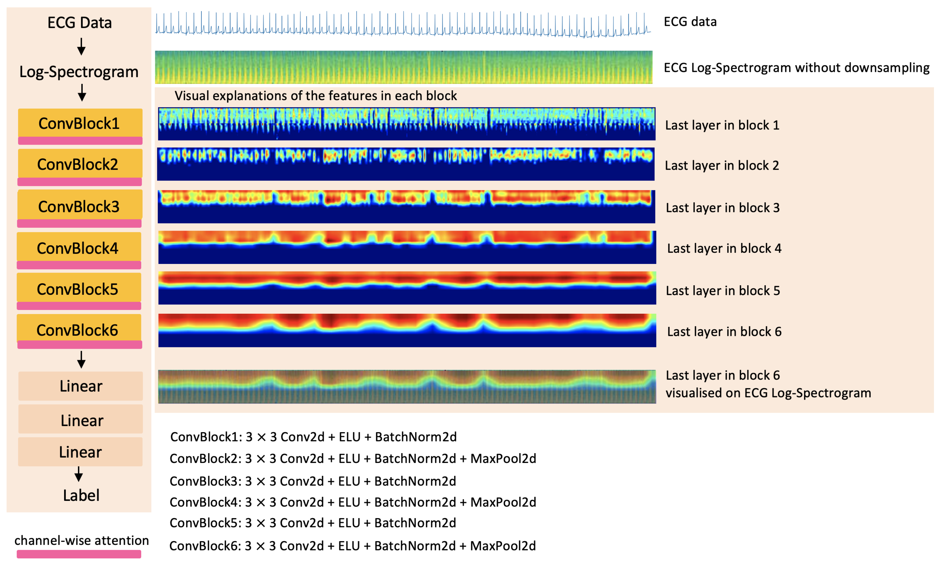
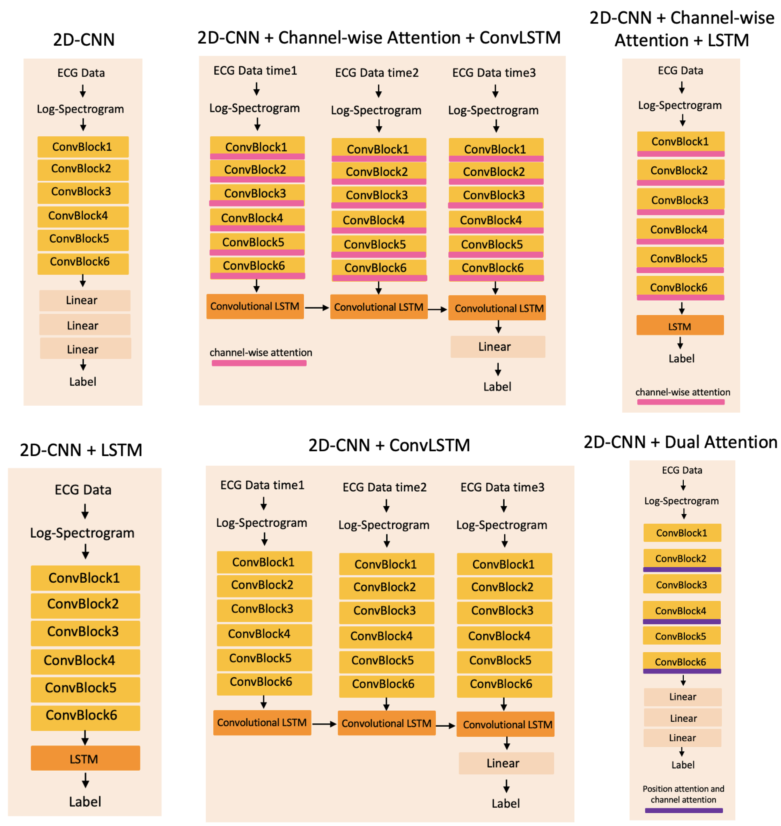
3. Method
- Data Preprocessing: ECG noise removal;
- Spectrogram analysis of single-lead ECG signal: Generated 2D log-spectrograms as inputs of the proposed method;
- Feature extraction with CNN: Feed the log-spectrograms into convolutional layers to extract features;
- Attention Mechanism: Model the inter-dependencies among the channel features of the convolutional layers.
3.1. Data Preprocessing
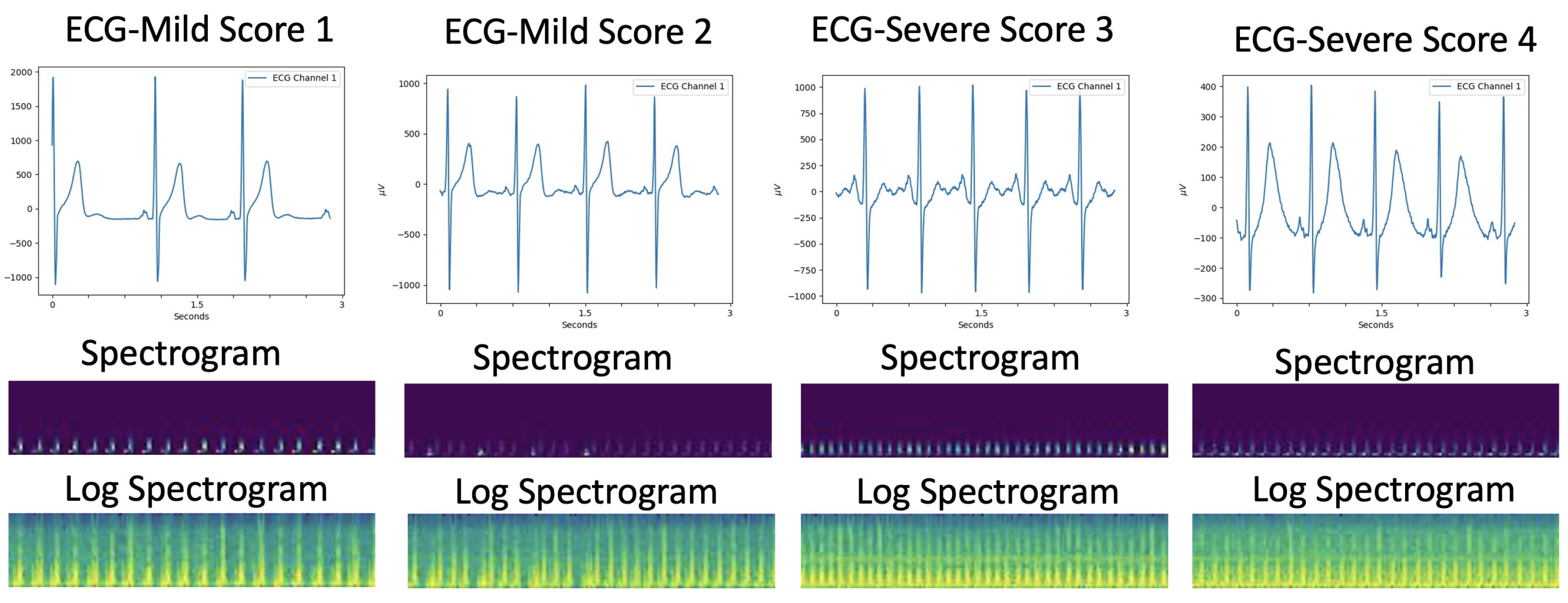
3.2. Logarithmic Spectrogram Generation
3.3. Attention-Based Network
3.3.1. Convolutional Layers
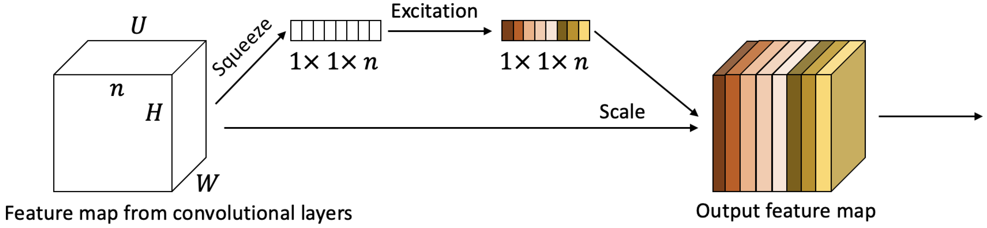
3.3.2. Channel-Wise Attention
3.3.3. Loss Function
4. Experiments
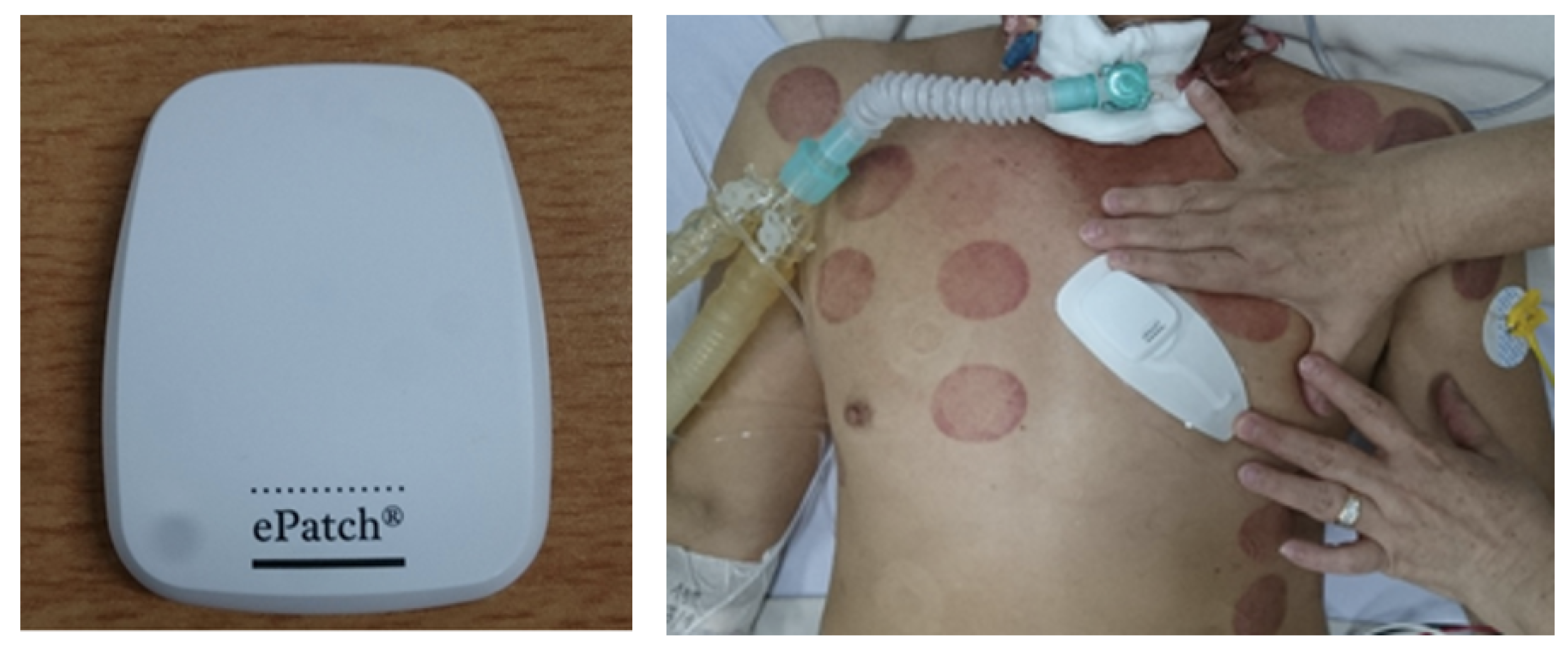
4.1. ECG Acquisition for Tetanus Patients
4.2. Implementation Details
4.2.1. Data Preprocessing
4.2.2. Training
4.3. Baseline Methods
4.4. Evaluation Metrics
5. Results and Discussion
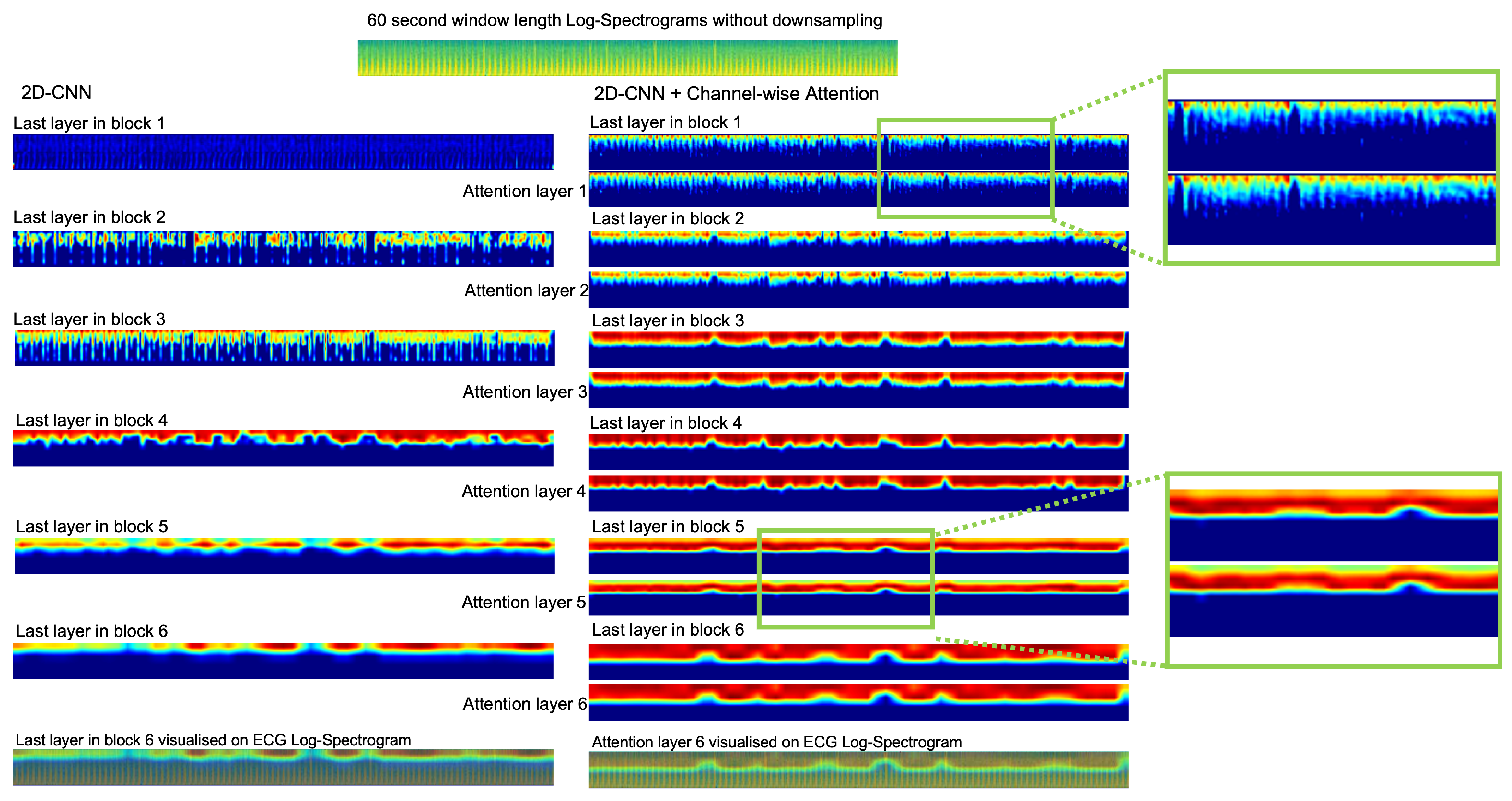
5.1. Attention Layers
5.2. Sequential Techniques
5.2.1. Recurrent Neural Network Layers
5.2.2. Convolutional LSTMs Model
5.3. 1D Convolutional Model
5.4. Downsample Spectrogram
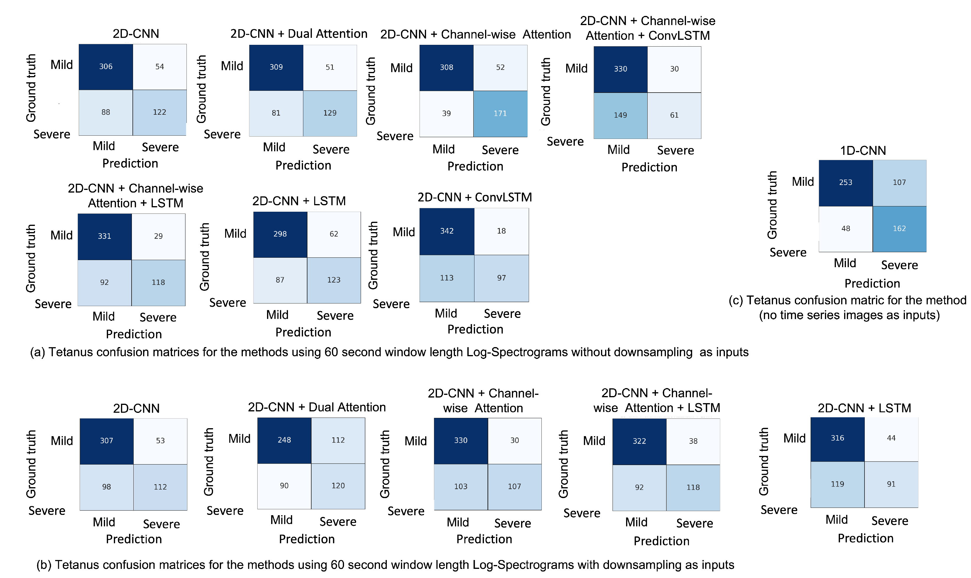
5.5. Misclassification
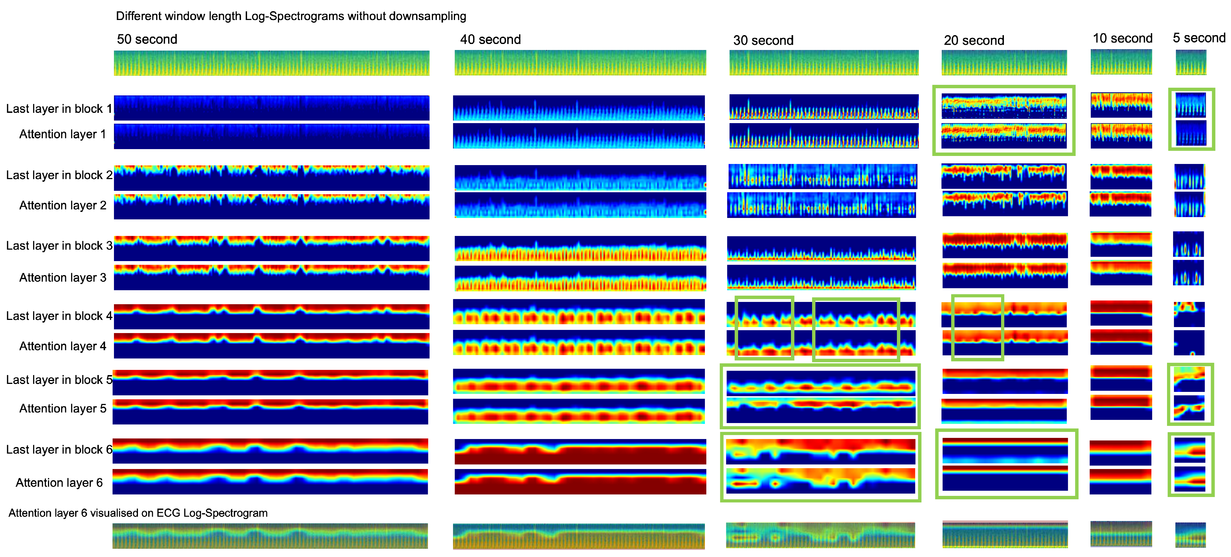
5.6. Window Length of Spectrogram
5.7. Traditional Machine Learning
6. Conclusions
Author Contributions
Funding
Institutional Review Board Statement
Informed Consent Statement
Data Availability Statement
Acknowledgments
Conflicts of Interest
References
- Thuy, D.B.; Campbell, J.I.; Thanh, T.T.; Thuy, C.T.; Loan, H.T.; Van Hao, N.; Minh, Y.L.; Van Tan, L.; Boni, M.F.; Thwaites, C.L. Tetanus in southern Vietnam: Current situation. Am. J. Trop. Med. Hyg. 2017, 96, 93. [Google Scholar] [CrossRef]
- Thwaites, C.; Yen, L.; Glover, C.; Tuan, P.; Nga, N.; Parry, J.; Loan, H.; Bethell, D.; Day, N.; White, N.; et al. Predicting the clinical outcome of tetanus: The tetanus severity score. Trop. Med. Int. Health 2006, 11, 279–287. [Google Scholar] [CrossRef]
- Van Hao, N.; Yen, L.M.; Davies-Foote, R.; Trung, T.N.; Duoc, N.V.T.; Trang, V.T.N.; Nhat, P.T.H.; Anh, N.T.K.; Lieu, P.T.; Thuy, T.T.D.; et al. The management of tetanus in adults in an intensive care unit in Southern Vietnam. Wellcome Open Res. 2021, 6, 107. [Google Scholar]
- Thwaites, C. Botulism and tetanus. Medicine 2017, 45, 739–742. [Google Scholar] [CrossRef]
- What are the Symptoms of Tetanus? Available online: https://healthclinics.superdrug.com/tetanus-symptoms/ (accessed on 21 August 2022).
- Duong, H.T.H.; Tadesse, G.A.; Nhat, P.T.H.; Van Hao, N.; Prince, J.; Duong, T.D.; Kien, T.T.; Nhat, L.T.H.; Van Tan, L.; Pugh, C.; et al. Heart rate variability as an indicator of autonomic nervous system disturbance in tetanus. Am. J. Trop. Med. Hyg. 2020, 102, 403. [Google Scholar] [CrossRef]
- Afshar, M.; Raju, M.; Ansell, D.; Bleck, T.P. Narrative review: Tetanus—A health threat after natural disasters in developing countries. Ann. Intern. Med. 2011, 154, 329–335. [Google Scholar] [CrossRef]
- The Importance of Diagnostic Tests in Fighting Infectious Diseases. Available online: https://www.lifechanginginnovation.org/medtech-facts/importance-diagnostic-tests-fighting-infectious-diseases.html (accessed on 21 August 2022).
- Trieu, H.T.; Anh, N.T.K.; Vuong, H.N.T.; Dao, T.; Hoa, N.T.X.; Tuong, V.N.C.; Dinh, P.T.; Wills, B.; Qui, P.T.; Van Tan, L.; et al. Long-term outcome in survivors of neonatal tetanus following specialist intensive care in Vietnam. BMC Infect. Dis. 2017, 17, 646. [Google Scholar] [CrossRef]
- Lam, P.K.; Trieu, H.T.; Lubis, I.N.D.; Loan, H.T.; Thuy, T.T.D.; Wills, B.; Parry, C.M.; Day, N.P.; Qui, P.T.; Yen, L.M.; et al. Prognosis of neonatal tetanus in the modern management era: An observational study in 107 Vietnamese infants. Int. J. Infect. Dis. 2015, 33, 7–11. [Google Scholar] [CrossRef]
- Cygankiewicz, I.; Zareba, W. Heart rate variability. Handb. Clin. Neurol. 2013, 117, 379–393. [Google Scholar]
- Task Force of the European Society of Cardiology the North American Society of Pacing Electrophysiology. Heart rate variability: Standards of measurement, physiological interpretation, and clinical use. Circulation 1996, 93, 1043–1065. [Google Scholar]
- Bolanos, M.; Nazeran, H.; Haltiwanger, E. Comparison of heart rate variability signal features derived from electrocardiography and photoplethysmography in healthy individuals. In Proceedings of the 2006 International Conference of the IEEE Engineering in Medicine and Biology Society, New York, NY, USA, 30 August–3 September 2006; pp. 4289–4294. [Google Scholar]
- Ghiasi, S.; Zhu, T.; Lu, P.; Hagenah, J.; Khanh, P.N.Q.; Hao, N.V.; Thwaites, L.; Clifton, D.A.; Consortium, V. Sepsis Mortality Prediction Using Wearable Monitoring in Low–Middle Income Countries. Sensors 2022, 22, 3866. [Google Scholar] [CrossRef] [PubMed]
- Lin, M.T.; Wang, J.K.; Lu, F.L.; Wu, E.T.; Yeh, S.J.; Lee, W.L.; Wu, J.M.; Wu, M.H. Heart rate variability monitoring in the detection of central nervous system complications in children with enterovirus infection. J. Crit. Care 2006, 21, 280–286. [Google Scholar] [CrossRef] [PubMed]
- Tadesse, G.A.; Zhu, T.; Thanh, N.L.N.; Hung, N.T.; Duong, H.T.H.; Khanh, T.H.; Van Quang, P.; Tran, D.D.; Yen, L.M.; Van Doorn, R.; et al. Severity detection tool for patients with infectious disease. Healthc. Technol. Lett. 2020, 7, 45–50. [Google Scholar] [CrossRef] [PubMed]
- Tadesse, G.A.; Javed, H.; Thanh, N.L.N.; Thi, H.D.H.; Thwaites, L.; Clifton, D.A.; Zhu, T. Multi-modal diagnosis of infectious diseases in the developing world. IEEE J. Biomed. Health Inform. 2020, 24, 2131–2141. [Google Scholar] [CrossRef]
- Kiyasseh, D.; Tadesse, G.A.; Thwaites, L.; Zhu, T.; Clifton, D. Plethaugment: Gan-based ppg augmentation for medical diagnosis in low-resource settings. IEEE J. Biomed. Health Inform. 2020, 24, 3226–3235. [Google Scholar] [CrossRef]
- Tutuko, B.; Nurmaini, S.; Tondas, A.E.; Rachmatullah, M.N.; Darmawahyuni, A.; Esafri, R.; Firdaus, F.; Sapitri, A.I. AFibNet: An Implementation of Atrial Fibrillation Detection with Convolutional Neural Network. BMC Med. Inform. Decis. Mak. 2021, 21, 216. [Google Scholar] [CrossRef]
- Kiranyaz, S.; Avci, O.; Abdeljaber, O.; Ince, T.; Gabbouj, M.; Inman, D.J. 1D convolutional neural networks and applications: A survey. Mech. Syst. Signal Process. 2021, 151, 107398. [Google Scholar] [CrossRef]
- Ullah, A.; Anwar, S.M.; Bilal, M.; Mehmood, R.M. Classification of arrhythmia by using deep learning with 2-D ECG spectral image representation. Remote Sens. 2020, 12, 1685. [Google Scholar] [CrossRef]
- Zihlmann, M.; Perekrestenko, D.; Tschannen, M. Convolutional recurrent neural networks for electrocardiogram classification. In Proceedings of the 2017 Computing in Cardiology (CinC), Rennes, France, 24–27 September 2017; pp. 1–4. [Google Scholar]
- Diker, A.; Cömert, Z.; Avcı, E.; Toğaçar, M.; Ergen, B. A novel application based on spectrogram and convolutional neural network for ecg classification. In Proceedings of the 2019 1st International Informatics and Software Engineering Conference (UBMYK), Ankara, Turkey, 6–7 November 2019; pp. 1–6. [Google Scholar]
- Liu, G.; Han, X.; Tian, L.; Zhou, W.; Liu, H. ECG quality assessment based on hand-crafted statistics and deep-learned S-transform spectrogram features. Comput. Methods Programs Biomed. 2021, 208, 106269. [Google Scholar] [CrossRef]
- Wu, Y.; Yang, F.; Liu, Y.; Zha, X.; Yuan, S. A comparison of 1-D and 2-D deep convolutional neural networks in ECG classification. arXiv 2018, arXiv:1810.07088. [Google Scholar]
- Guo, M.H.; Xu, T.X.; Liu, J.J.; Liu, Z.N.; Jiang, P.T.; Mu, T.J.; Zhang, S.H.; Martin, R.R.; Cheng, M.M.; Hu, S.M. Attention Mechanisms in Computer Vision: A Survey. arXiv 2021, arXiv:2111.07624. [Google Scholar] [CrossRef]
- Woo, S.; Park, J.; Lee, J.Y.; Kweon, I.S. Cbam: Convolutional block attention module. In Proceedings of the European Conference on Computer Vision (ECCV), Munich, Germany, 8–14 September 2018; pp. 3–19. [Google Scholar]
- Hu, J.; Shen, L.; Sun, G. Squeeze-and-excitation networks. In Proceedings of the IEEE Conference on Computer Vision and Pattern Recognition, Salt Lake City, UT, USA, 18–23 June 2018; pp. 7132–7141. [Google Scholar]
- Wang, X.; Girshick, R.; Gupta, A.; He, K. Non-local neural networks. In Proceedings of the IEEE Conference on Computer Vision and Pattern Recognition, Salt Lake City, UT, USA, 18–23 June 2018; pp. 7794–7803. [Google Scholar]
- Du, W.; Wang, Y.; Qiao, Y. Recurrent spatial-temporal attention network for action recognition in videos. IEEE Trans. Image Process. 2017, 27, 1347–1360. [Google Scholar] [CrossRef] [PubMed]
- Hochreiter, S.; Schmidhuber, J. Long short-term memory. Neural Comput. 1997, 9, 1735–1780. [Google Scholar] [PubMed]
- Selvaraju, R.R.; Cogswell, M.; Das, A.; Vedantam, R.; Parikh, D.; Batra, D. Grad-cam: Visual explanations from deep networks via gradient-based localization. In Proceedings of the International Conference on Computer Vision, Venice, Italy, 22–29 October 2017; pp. 618–626. [Google Scholar]
- Byeon, Y.H.; Kwak, K.C. Pre-configured deep convolutional neural networks with various time-frequency representations for biometrics from ECG signals. Appl. Sci. 2019, 9, 4810. [Google Scholar]
- Virtanen, P.; Gommers, R.; Oliphant, T.E.; Haberland, M.; Reddy, T.; Cournapeau, D.; Burovski, E.; Peterson, P.; Weckesser, W.; Bright, J.; et al. SciPy 1.0: Fundamental Algorithms for Scientific Computing in Python. Nat. Methods 2020, 17, 261–272. [Google Scholar] [CrossRef] [Green Version]
- Goodfellow, I.; Bengio, Y.; Courville, A. Deep Learning; MIT press: Cambridge, MA, USA, 2016. [Google Scholar]
- ePatch™. The World’s Most Wearable Holter Monitor. Available online: https://www.gobio.com/clinical-research/cardiac-safety/epatch/ (accessed on 21 August 2022).
- Dorthe Bodholt, S.; Helge Bjarup Dissing, S.; Ingeborg Helbech, H.; Kenneth, E.; Poul, J.; Karsten, H. Available online: https://backend.orbit.dtu.dk/ws/portalfiles/portal/102966188/ePatch_A_Clinical_Overview_DTU_Technical_Report.pdf (accessed on 21 August 2022).
- Van, H.M.T.; Van Hao, N.; Quoc, K.P.N.; Hai, H.B.; Yen, L.M.; Nhat, P.T.H.; Duong, H.T.H.; Thuy, D.B.; Zhu, T.; Greeff, H.; et al. Vital sign monitoring using wearable devices in a Vietnamese intensive care unit. BMJ Innov. 2021, 7. [Google Scholar] [CrossRef]
- Fu, J.; Liu, J.; Tian, H.; Li, Y.; Bao, Y.; Fang, Z.; Lu, H. Dual attention network for scene segmentation. In Proceedings of the IEEE/CVF Conference on Computer Vision and Pattern Recognition, Long Beach, CA, USA, 15–20 June 2019; pp. 3146–3154. [Google Scholar]
- Lu, P.; Qiu, H.; Qin, C.; Bai, W.; Rueckert, D.; Noble, J.A. Going deeper into cardiac motion analysis to model fine spatio-temporal features. In Proceedings of the Annual Conference on Medical Image Understanding and Analysis; Springer: Berlin/Heidelberg, Germany, 2020; pp. 294–306. [Google Scholar]
- Xingjian, S.; Chen, Z.; Wang, H.; Yeung, D.Y.; Wong, W.K.; Woo, W.c. Convolutional LSTM network: A machine learning approach for precipitation nowcasting. In Proceedings of the Advances in Neural Information Processing Systems, Montreal, QC, Canada, 7–12 December 2015; pp. 802–810. [Google Scholar]
- Breiman, L. Random forests. Mach. Learn. 2001, 45, 5–32. [Google Scholar] [CrossRef]
- Lu, P.; Barazzetti, L.; Chandran, V.; Gavaghan, K.; Weber, S.; Gerber, N.; Reyes, M. Highly accurate facial nerve segmentation refinement from CBCT/CT imaging using a super-resolution classification approach. IEEE Trans. Biomed. Eng. 2017, 65, 178–188. [Google Scholar] [CrossRef]
- Vest, A.N.; Da Poian, G.; Li, Q.; Liu, C.; Nemati, S.; Shah, A.J.; Clifford, G.D. An open source benchmarked toolbox for cardiovascular waveform and interval analysis. Physiol. Meas. 2018, 39, 105004. [Google Scholar]
- Vollmer, M. HRVTool—An Open-Source Matlab Toolbox for Analyzing Heart Rate Variability. In Proceedings of the Computing in Cardiology 2019, Singapore, 8–11 September 2019; Volume 46. [Google Scholar] [CrossRef]
- Vollmer, M. A robust, simple and reliable measure of heart rate variability using relative RR intervals. In Proceedings of the 2015 Computing in Cardiology Conference (CinC), Nice, France, 6–9 September 2015; pp. 609–612. [Google Scholar] [CrossRef]
- Heart Rate Variability Analysis. Available online: https://pypi.org/project/hrv-analysis/ (accessed on 21 August 2022).
- Seven ECG Heartbeat Detection Algorithms and Heartrate Variability Analysis. Available online: https://www.ecdc.europa.eu/en/tetanus/facts (accessed on 21 August 2022).
- Touvron, H.; Cord, M.; Douze, M.; Massa, F.; Sablayrolles, A.; Jégou, H. Training data-efficient image transformers & distillation through attention. In Proceedings of the International Conference on Machine Learning, PMLR, Virtual, 18–24 July 2021; pp. 10347–10357. Available online: https://proceedings.mlr.press/v139/touvron21a.html (accessed on 21 August 2022).
- Khan, S.; Naseer, M.; Hayat, M.; Zamir, S.W.; Khan, F.S.; Shah, M. Transformers in vision: A survey. ACM Comput. Surv. CSUR 2021. [Google Scholar] [CrossRef]
- Dosovitskiy, A.; Beyer, L.; Kolesnikov, A.; Weissenborn, D.; Zhai, X.; Unterthiner, T.; Dehghani, M.; Minderer, M.; Heigold, G.; Gelly, S.; et al. An image is worth 16x16 words: Transformers for image recognition at scale. arXiv 2020, arXiv:2010.11929. [Google Scholar]
- Lopes, R.G.; Fenu, S.; Starner, T. Data-free knowledge distillation for deep neural networks. arXiv 2017, arXiv:1710.07535. [Google Scholar]
- Gou, J.; Yu, B.; Maybank, S.J.; Tao, D. Knowledge distillation: A survey. Int. J. Comput. Vis. 2021, 129, 1789–1819. [Google Scholar]


| 60 s Window Length Log-Spectrogram without Downsampling | ||||||
| Method | F1 Score | Precision | Recall | Specificity | Accuracy | AUC |
| 2D-CNN | 0.61 ± 0.14 | 0.68 ± 0.07 | 0.57 ± 0.19 | 0.85 ± 0.02 | 0.75 ± 0.07 | 0.72 ± 0.09 |
| 2D-CNN + Dual Attention | 0.65 ± 0.19 | 0.71 ± 0.17 | 0.61 ± 0.21 | 0.86 ± 0.09 | 0.76 ± 0.11 | 0.74 ± 0.13 |
| 2D-CNN + Channel-wise Attention | 0.79 ± 0.03 | 0.78 ± 0.08 | 0.82 ± 0.05 | 0.85 ± 0.08 | 0.84 ± 0.04 | 0.84 ± 0.03 |
| 2D-CNN + LSTM | 0.61 ± 0.15 | 0.71 ± 0.16 | 0.59 ± 0.20 | 0.83 ± 0.17 | 0.74 ± 0.10 | 0.71 ± 0.10 |
| 2D-CNN + ConvLSTM | 0.52 ± 0.32 | 0.77 ± 0.23 | 0.46 ± 0.33 | 0.95 ± 0.04 | 0.77 ± 0.11 | 0.71 ± 0.15 |
| 2D-CNN + Channel-wise Attention + ConvLSTM | 0.38 ± 0.17 | 0.67 ± 0.10 | 0.29 ± 0.16 | 0.92 ± 0.06 | 0.68 ± 0.05 | 0.60 ± 0.06 |
| 2D-CNN + Channel-wise Attention + LSTM | 0.59 ± 0.32 | 0.70 ± 0.34 | 0.56 ± 0.34 | 0.92 ± 0.92 | 0.79 ± 0.12 | 0.74 ± 0.16 |
| No Time Series Images | ||||||
| Method | F1 Score | Precision | Recall | Specificity | Accuracy | AUC |
| 1D-CNN | 0.65 ± 0.14 | 0.61 ± 0.05 | 0.77 ± 0.25 | 0.70 ± 0.13 | 0.73 ± 0.05 | 0.74 ± 0.08 |
| 60 s Window Length Log-Spectrogram with Downsampling | ||||||
|---|---|---|---|---|---|---|
| Method | F1 Score | Precision | Recall | Specificity | Accuracy | AUC |
| 2D-CNN | 0.58 ± 0.16 | 0.68 ± 0.05 | 0.53 ± 0.19 | 0.85 ± 0.06 | 0.74 ± 0.05 | 0.69 ± 0.07 |
| 2D-CNN + Dual Attention | 0.54 ± 0.08 | 0.57 ± 0.17 | 0.57 ± 0.21 | 0.69 ± 0.23 | 0.65 ± 0.09 | 0.63 ± 0.06 |
| 2D-CNN + Channel-wise Attention | 0.60 ± 0.10 | 0.82 ± 0.10 | 0.51 ± 0.16 | 0.92 ± 0.08 | 0.77 ± 0.30 | 0.71 ± 0.05 |
| 2D-CNN + LSTM | 0.52 ± 0.12 | 0.67 ± 0.03 | 0.43 ± 0.14 | 0.88 ± 0.03 | 0.71 ± 0.04 | 0.66 ± 0.06 |
| 2D-CNN + Channel-wise Attention + LSTM | 0.63 ± 0.13 | 0.75 ± 0.05 | 0.56 ± 0.19 | 0.89 ± 0.04 | 0.77 ± 0.05 | 0.73 ± 0.08 |
| The Proposed Method (Spectrograms without Downsampling) | ||||||
|---|---|---|---|---|---|---|
| Window Duration | F1 Score | Precision | Recall | Specificity | Accuracy | AUC |
| 50 s | 0.81 ± 0.05 | 0.81 ± 0.06 | 0.82 ± 0.04 | 0.88 ± 0.04 | 0.86 ± 0.04 | 0.85 ± 0.04 |
| 40 s | 0.80 ± 0.04 | 0.84 ± 0.08 | 0.77 ± 0.07 | 0.91 ± 0.05 | 0.86 ± 0.03 | 0.84 ± 0.03 |
| 30 s | 0.74 ± 0.05 | 0.79 ± 0.07 | 0.79 ± 0.07 | 0.87 ± 0.06 | 0.84 ± 0.04 | 0.83 ± 0.04 |
| 20 s | 0.79 ± 0.05 | 0.80 ± 0.08 | 0.78 ± 0.07 | 0.88 ± 0.07 | 0.84 ± 0.04 | 0.83 ± 0.04 |
| 10 s | 0.55 ± 0.33 | 0.74 ± 0.16 | 0.45 ± 0.38 | 0.90 ± 0.06 | 0.77 ± 0.12 | 0.72 ± 0.17 |
| 5 s | 0.43 ± 0.32 | 0.98 ± 0.02 | 0.34 ± 0.29 | 0.99 ± 0.01 | 0.75 ± 0.10 | 0.67 ± 0.14 |
| Parameters | |
|---|---|
| HRV time domain features | |
| mean_nni | mean of RR-intervals |
| sdnn | standard deviation of RR-intervals |
| sdsd | standard deviation of differences between adjacent RR-intervals |
| rmssd | square root of the mean of the sum of the squares of differences between adjacent NN-intervals |
| mean_hr | mean Heart Rate |
| max_hr | max heart rate |
| min_hr | min heart rate |
| std_hr | standard deviation of heart rate |
| 60 s Window Length Log-Spectrogram | ||||||
| Method | F1 Score | Precision | Recall | Specificity | Accuracy | AUC |
| 2D-CNN + Channel-wise Attention | 0.79 ± 0.03 | 0.78 ± 0.08 | 0.82 ± 0.05 | 0.85 ± 0.08 | 0.84 ± 0.04 | 0.84 ± 0.03 |
| No Time Series Images | ||||||
| Method | F1 Score | Precision | Recall | Specificity | Accuracy | AUC |
| Random Forest (HRV time domain features) | 0.81 ± 0.00 | 0.77 ± 0.00 | 0.85 ± 0.01 | 0.85 ± 0.00 | 0.85 ± 0.00 | 0.80 ± 0.00 |
Publisher’s Note: MDPI stays neutral with regard to jurisdictional claims in published maps and institutional affiliations. |
© 2022 by the authors. Licensee MDPI, Basel, Switzerland. This article is an open access article distributed under the terms and conditions of the Creative Commons Attribution (CC BY) license (https://creativecommons.org/licenses/by/4.0/).
Share and Cite
Lu, P.; Ghiasi, S.; Hagenah, J.; Hai, H.B.; Hao, N.V.; Khanh, P.N.Q.; Khoa, L.D.V.; VITAL Consortium; Thwaites, L.; Clifton, D.A.; et al. Classification of Tetanus Severity in Intensive-Care Settings for Low-Income Countries Using Wearable Sensing. Sensors 2022, 22, 6554. https://doi.org/10.3390/s22176554
Lu P, Ghiasi S, Hagenah J, Hai HB, Hao NV, Khanh PNQ, Khoa LDV, VITAL Consortium, Thwaites L, Clifton DA, et al. Classification of Tetanus Severity in Intensive-Care Settings for Low-Income Countries Using Wearable Sensing. Sensors. 2022; 22(17):6554. https://doi.org/10.3390/s22176554
Chicago/Turabian StyleLu, Ping, Shadi Ghiasi, Jannis Hagenah, Ho Bich Hai, Nguyen Van Hao, Phan Nguyen Quoc Khanh, Le Dinh Van Khoa, VITAL Consortium, Louise Thwaites, David A. Clifton, and et al. 2022. "Classification of Tetanus Severity in Intensive-Care Settings for Low-Income Countries Using Wearable Sensing" Sensors 22, no. 17: 6554. https://doi.org/10.3390/s22176554