
Measuring Relative Wind Speeds in Stratospheric Balloons with Cup Anemometers: The TASEC-Lab Mission

 ,
,  , , and
Abstract
:1. Introduction
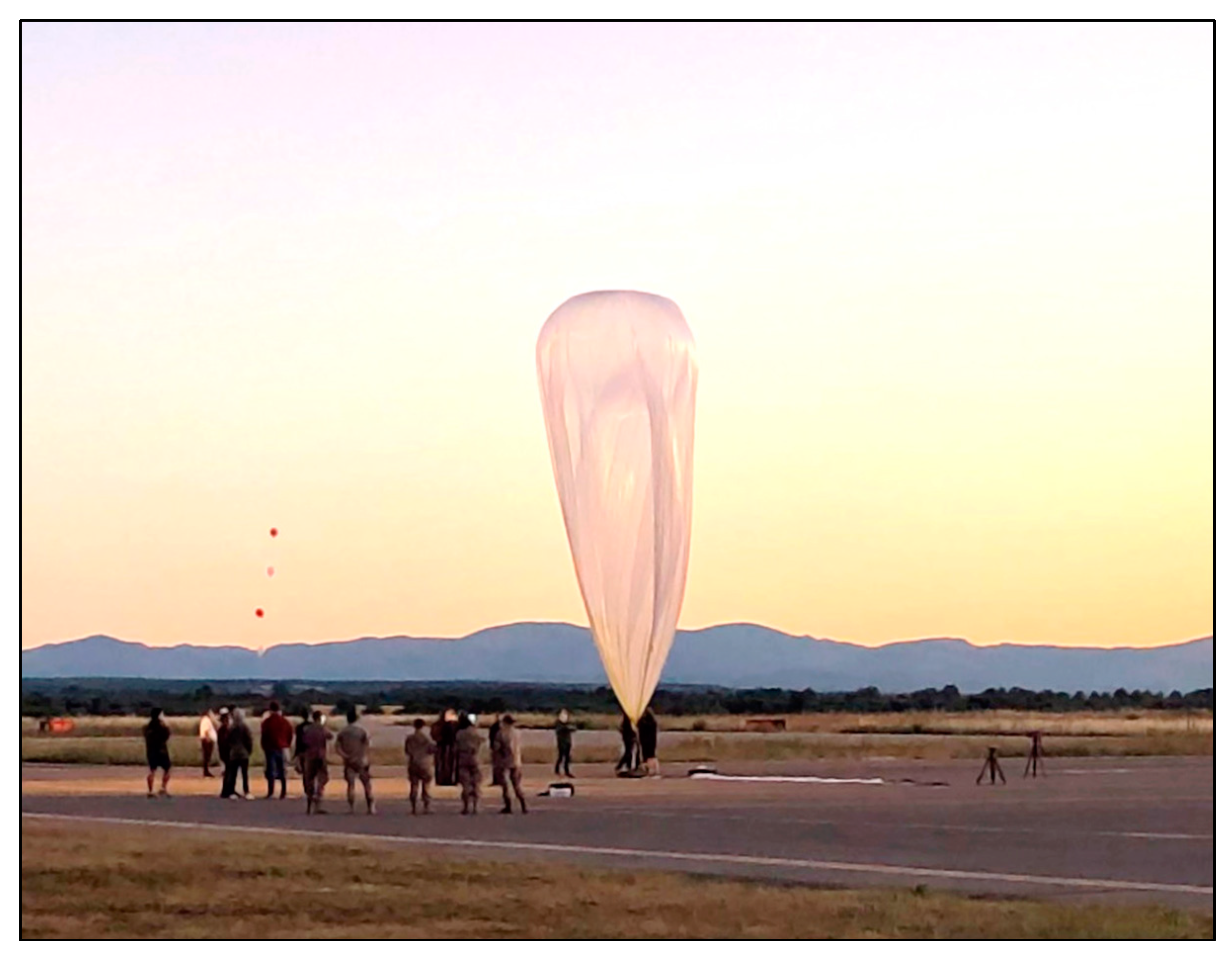
The TASEC-Lab Mission
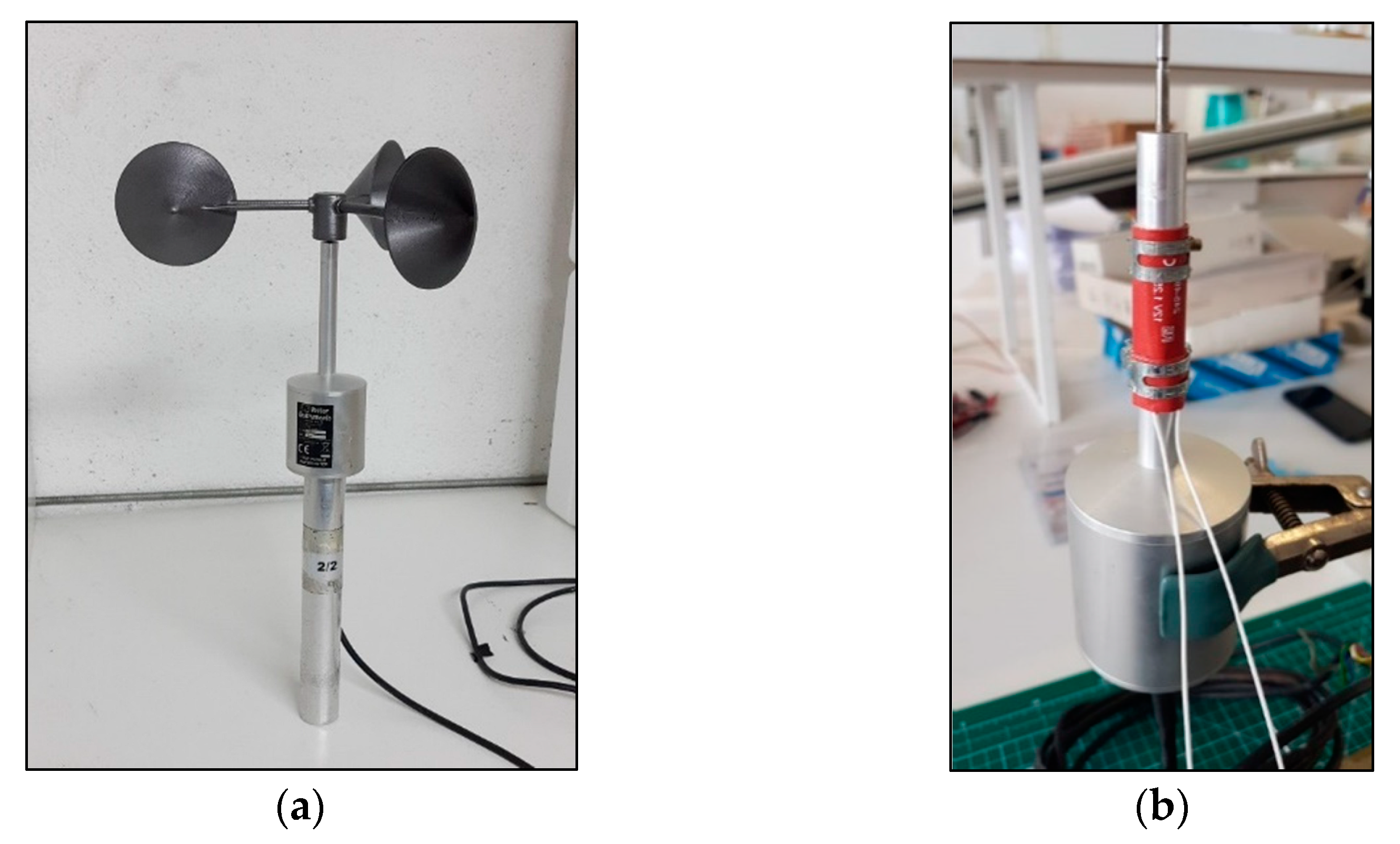
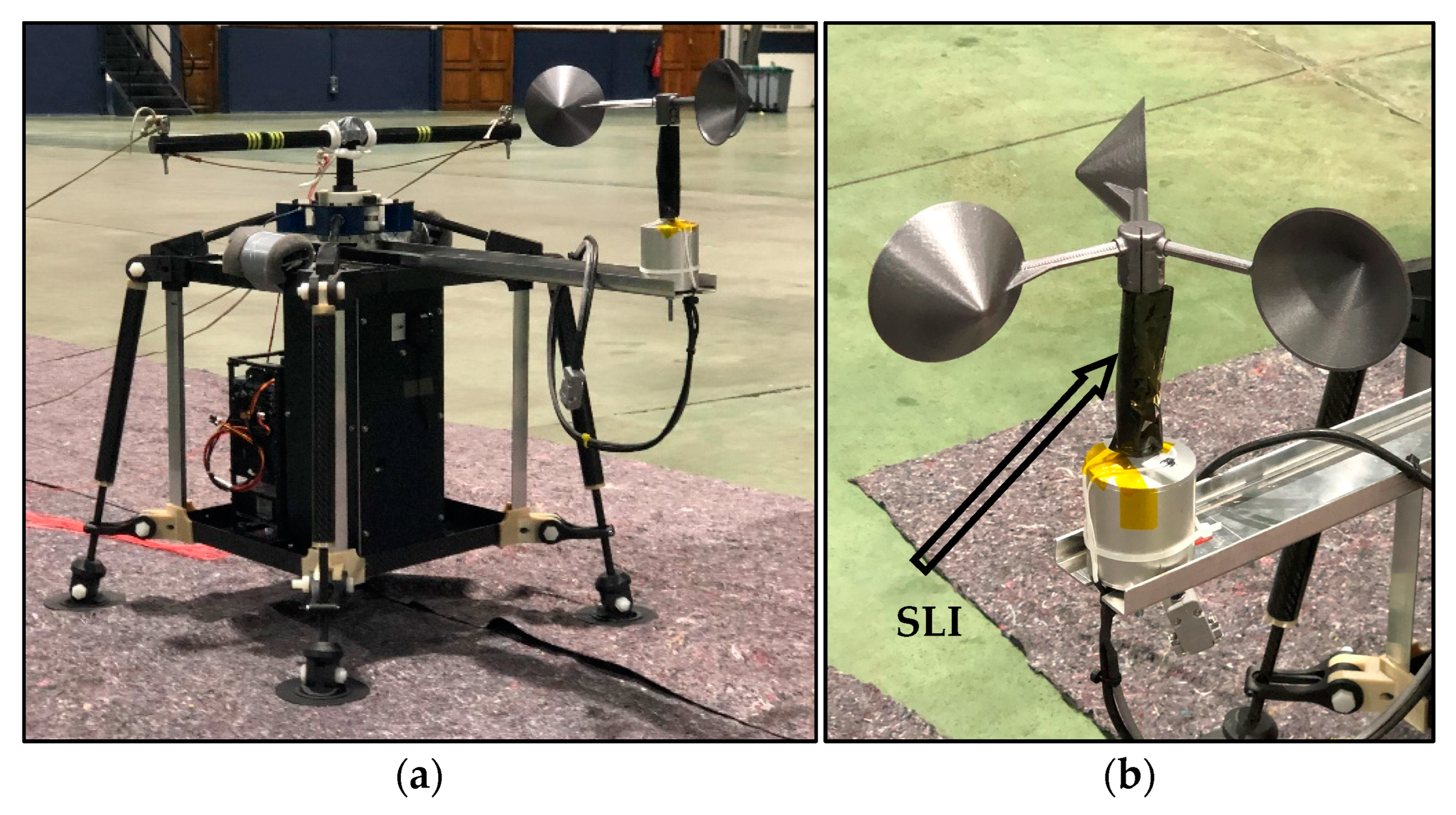
2. Materials and Methods
3. Results and Discussion
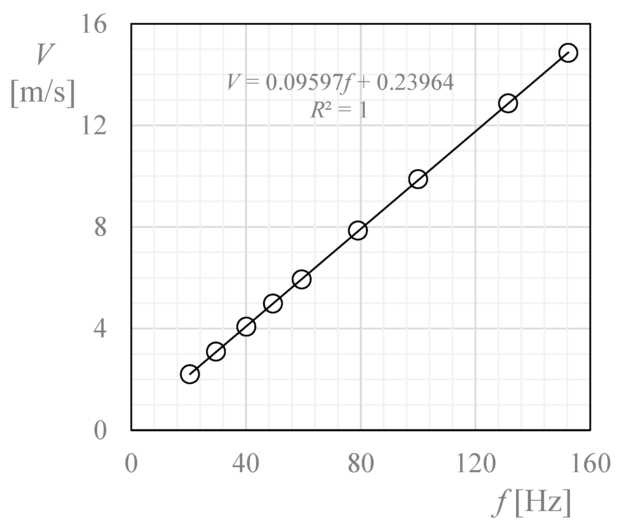
- use the transfer function of the sensor (i.e., the calibration constants, A and B; see Equation (5) and Figure 3 to obtain the wind speed at ground level, Vref, in relation to the output frequency, f, and then to
- translate that wind speed at ground level into a local wind speed (i.e., at the proper altitude), V.
4. Conclusions
- It is possible to use cup anemometers in stratospheric balloon missions. This instrument is an adequate alternative to the sonic anemometer, whose measurements can be affected by the low air densities at high altitudes above ground.
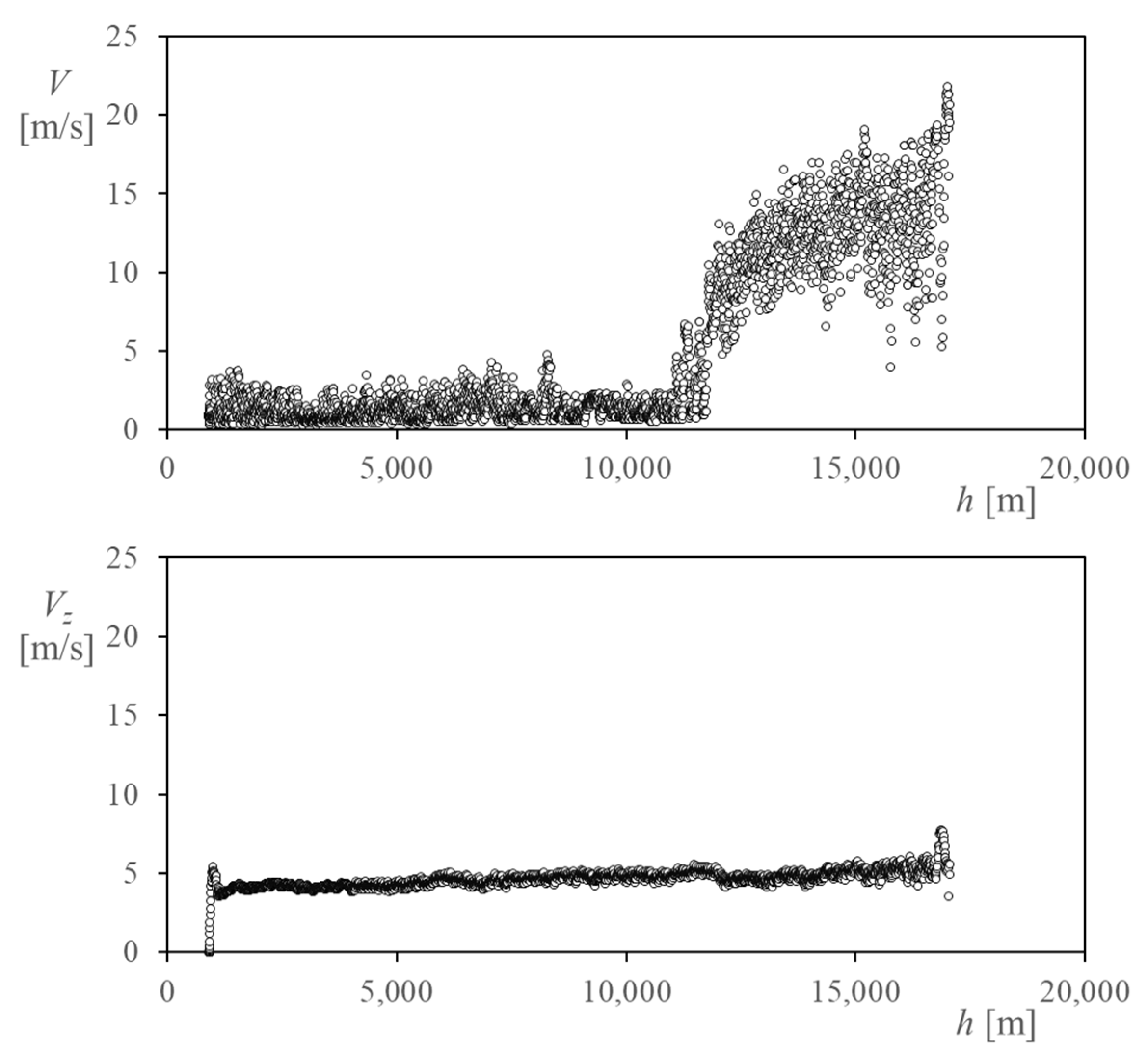
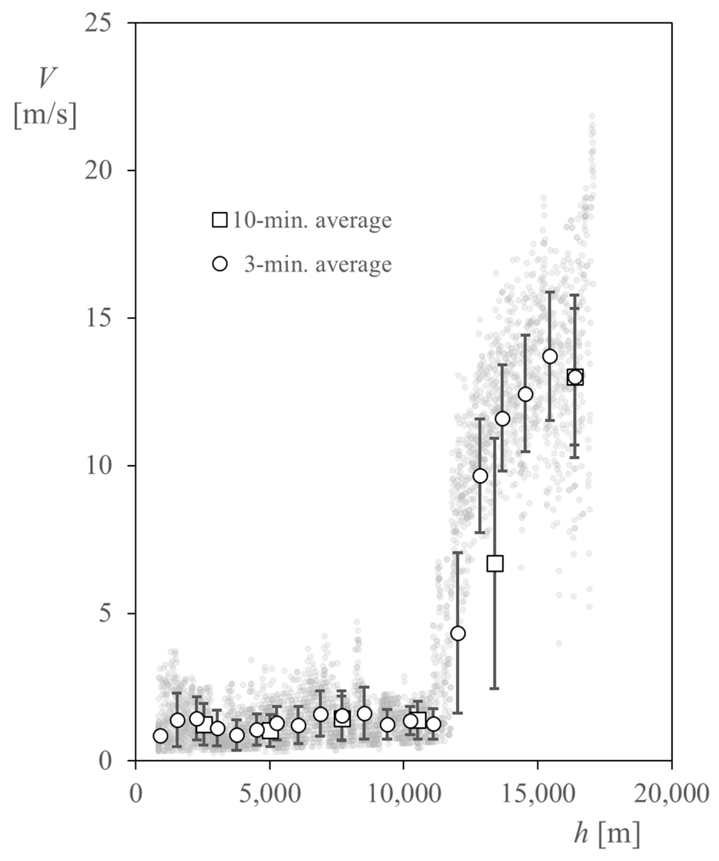
- Large wind speeds (up to 22 m/s) were measured beyond the tropopause, the deviation of these measurements being much larger than those of the troposphere.
- The highest variations of the horizontal wind speed were measured at the tropopause (at 12 km altitude), as expected.
Author Contributions
Funding
Institutional Review Board Statement
Informed Consent Statement
Data Availability Statement
Acknowledgments
Conflicts of Interest
References
- Parkinson, G.V. Wind-Induced Instability of Structures. Philos. Trans. R. Soc. London. Ser. A Math. Phys. Sci. 1971, 269, 395–409. [Google Scholar] [CrossRef]
- Blaylock, G. Putnam’s Power from the Wind. IEE Proc. C Gener. Transm. Distrib. 1983, 130, 59. [Google Scholar] [CrossRef]
- Justus, C.G. Winds and Wind System Performance; Franklin Institute Press: Philadelphia, PA, USA, 1978. [Google Scholar]
- Moor, G.D.; Beukes, H.J. Maximum Power Point Trackers for Wind Turbines. PESC Rec.-IEEE Annu. Power Electron. Spec. Conf. 2004, 3, 2044–2049. [Google Scholar] [CrossRef]
- Robinson, T.R. On a New Anemometer. Proc. R. Irish Acad. 1847, 4, 566–572. [Google Scholar]
- Robinson, T.R. XXV. On the Determination of the Constants of the Cup Anemometer by Experiments with a Whirling Machine—Part II. Philos. Trans. R. Soc. Lond. 1880, 171, 1055–1070. [Google Scholar] [CrossRef] [Green Version]
- Robinson, T.R., II. On the Determination of the Constants of the Cup Anemometer by Experiments with a Whirling Machine. Proc. R. Soc. Lond. 1878, 27, 286–289. [Google Scholar] [CrossRef]
- Pindado, S.; Cubas, J.; Sorribes-Palmer, F. The Cup Anemometer, A Fundamental Meteorological Instrument for the Wind Energy Industry. Research at the IDR/UPM Institute. Sensors 2014, 14, 21418–21452. [Google Scholar] [CrossRef] [Green Version]
- Coquilla, R.V.; Obermeier, J.; White, B.R. Calibration Procedures and Uncertainty in Wind Power Anemometers. Wind. Eng. 2016, 31, 303. [Google Scholar] [CrossRef]
- Wellman, J.B. A Folding Rotating Cup Anemometer. In Space Programs Summary 37-53, Vol. III. Supporting Research and Advanced Development for the Period August 1 to September 30, 1968; NASA Jet Propulsion Laboratory, California Institute of Technology: Pasadena, CA, USA, 1968; pp. 133–143. [Google Scholar]
- Lorenz, R.D. Surface Winds on Venus: Probability Distribution from in-Situ Measurements. Icarus 2016, 264, 311–315. [Google Scholar] [CrossRef]
- Brevoort, M.J.; Joyner, U.T. Experimental Investigation of the Robinson-Type Cup Anemometer. U.S. Patent No. NACA-TR-513, 1 January 1936. [Google Scholar]
- Schubauer, G.B.; Mason, M.A. Performance Characteristics of a Water Current Meter in Water and in Air. J. Res. Natl. Bur. Stand. (1934) 1937, 18, 351–360. [Google Scholar] [CrossRef]
- Ramos-Cenzano, Á.; López-Núñez, E.; Alfonso-Corcuera, D.; Ogueta-Gutiérrez, M.; Pindado, S. On Cup Anemometer Performance at High Altitude above Ground. Flow Meas. Instrum. 2021, 79, 101956. [Google Scholar] [CrossRef]
- Siebert, H.; Wendisch, M.; Conrath, T.; Teichmann, U.; Heintzenberg, J. A New Tethered Balloon-Borne Payload for Fine-Scale Observations in the Cloudy Boundary Layer. Boundary-Layer Meteorol. 2003, 106, 461–482. [Google Scholar] [CrossRef]
- Tjernström, M.; Leck, C.; Persson, P.O.G.; Jensen, M.L.; Oncley, S.P.; Targino, A. The Summertime Arctic Atmosphere: Meteorological Measurements during the Arctic Ocean Experiment 2001. Bull. Am. Meteorol. Soc. 2004, 85, 1305–1322. [Google Scholar] [CrossRef]
- Canut, G.; Couvreux, F.; Lothon, M.; Legain, D.; Piguet, B.; Lampert, A.; Maurel, W.; Moulin, E. Turbulence Fluxes and Variances Measured with a Sonic Anemometer Mounted on a Tethered Balloon. Atmos. Meas. Tech. 2016, 9, 4375–4386. [Google Scholar] [CrossRef] [Green Version]
- Egerer, U.; Gottschalk, M.; Siebert, H.; Ehrlich, A.; Wendisch, M. The New BELUGA Setup for Collocated Turbulence and Radiation Measurements Using a Tethered Balloon: First Applications in the Cloudy Arctic Boundary Layer. Atmos. Meas. Tech. 2019, 12, 4019–4038. [Google Scholar] [CrossRef] [Green Version]
- Maruca, B.A.; Marino, R.; Sundkvist, D.; Godbole, N.H.; Constantin, S.; Carbone, V.; Zimmerman, H. Overview of and First Observations from the TILDAE High-Altitude Balloon Mission. Atmos. Meas. Tech. 2017, 10, 1595–1607. [Google Scholar] [CrossRef]
- Torochkov, V.Y.; Surazhskiy, D.Y. Measuring Average Wind Speed (No. FTD-HT-23-341-69). Foreign Technol. Div. Wright-Patterson AFB OH 1969. Available online: https://apps.dtic.mil/sti/citations/AD0696229 (accessed on 25 June 2022).
- Hayashi, T. Dynamic Response of a Cup Anemometer. J. Atmos. Ocean. Technol. 1987, 4, 281–287. [Google Scholar] [CrossRef] [Green Version]
- COPPIN, P.A. An Examination of cup anemometer overspeeding. Meteorol. Rundsch. 1982, 35, 1–11. [Google Scholar]
- Wyngaard, J.C. Cup, Propeller, Vane, and Sonic Anemometers in Turbulence Research. Annu. Rev. Fluid Mech. 2003, 13, 399–423. [Google Scholar] [CrossRef]
- Pedersen, T.F. Characterisation and Classification of Risø P2546 Cup Anemometer; Risø DTU-National Laboratory for Sustainable Energy: Roskilde, Denmark, 2004. [Google Scholar]
- Sanz-Andrés, Á.; Pindado, S.; Sorribes-Palmer, F. Mathematical Analysis of the Effect of Rotor Geometry on Cup Anemometer Response. Sci. World J. 2014, 2014, 537813. [Google Scholar] [CrossRef]
- Frenzen, P. Fast Response Cup Anemometers for Atmospheric Turbulence Research. In Proceedings of the 8th Symposium on Turbulence and Diffusion, San Diego, CA, USA, 25–29 April 1988; pp. 112–115. [Google Scholar]
- Ligęza, P.; Jamróz, P.; Ostrogórski, P. Methods for Dynamic Behavior Improvement of Tachometric and Thermal Anemometers by Active Control. Measurement 2020, 166, 108147. [Google Scholar] [CrossRef]
- Ligęza, P. Method of Testing Fast-Changing and Pulsating Flows by Means of a Hot-Wire Anemometer with Simultaneous Measurement of Voltage and Current of the Sensor. Measurement 2022, 187, 110291. [Google Scholar] [CrossRef]
- Ligęza, P. Dynamic Error Correction Method in Tachometric Anemometers for Measurements of Wind Energy. Energies 2022, 15, 4132. [Google Scholar] [CrossRef]
- Kremic, T.; Hibbitts, K.; Young, E.; Landis, R.; Noll, K.; Baines, K. Assessing the Potential of Stratospheric Balloons for Planetary Science. In Proceedings of the 2013 IEEE Aerospace Conference, Big Sky, MT, USA, 2–9 March 2013. [Google Scholar] [CrossRef] [Green Version]
- Stern, S.A.; Poynter, J.; MacCallum, T. World View Stratospheric Ballooning Capabilities, Research, and Commercial Applications. In Proceedings of the 2017 IEEE Aerospace Conference, Big Sky, MT, USA, 4–11 March 2017. [Google Scholar] [CrossRef]
- Marzioli, P.; Frezza, L.; Curianò, F.; Pellegrino, A.; Gianfermo, A.; Angeletti, F.; Arena, L.; Cardona, T.; Valdatta, M.; Santoni, F.; et al. Experimental Validation of VOR (VHF Omni Range) Navigation System for Stratospheric Flight. Acta Astronaut. 2021, 178, 423–431. [Google Scholar] [CrossRef]
- Gemignani, M.; Marcuccio, S. Dynamic Characterization of a High-Altitude Balloon during a Flight Campaign for the Detection of ISM Radio Background in the Stratosphere. Aerospace 2021, 8, 21. [Google Scholar] [CrossRef]
- González-Bárcena, D.; Fernández-Soler, A.; Pérez-Grande, I.; Sanz-Andrés, Á. Real Data-Based Thermal Environment Definition for the Ascent Phase of Polar-Summer Long Duration Balloon Missions from Esrange (Sweden). Acta Astronaut. 2020, 170, 235–250. [Google Scholar] [CrossRef]
- Ayape, F.; Muntean, V.; Engineer, T.; Engineer, T. Experiments of the Prototype for a Stratospheric Balloon-Borne Heat Transfer Laboratory. In Proceedings of the 50th International Conference on Environmental Systems, Madrid, Spain, 12–15 July 2021. [Google Scholar]
- González-Llana, A.; González-Bárcena, D.; Pérez-Grande, I.; Sanz-Andrés, Á. Selection of Extreme Environmental Conditions, Albedo Coefficient and Earth Infrared Radiation, for Polar Summer Long Duration Balloon Missions. Acta Astronaut. 2018, 148, 276–284. [Google Scholar] [CrossRef]
- González-Bárcena, D.; Peinado-Pérez, L.; Fernández-Soler, A.; Pérez-Muñoz, Á.G.; Álvarez-Romero, J.M.; Ayape, F.; Martín, J.; Bermejo-Ballesteros, J.; Porras-Hermoso, Á.L.; Alfonso-Corcuera, D.; et al. TASEC-Lab: A COTS-Based CubeSat-like University Experiment for Characterizing the Convective Heat Transfer in Stratospheric Balloon Missions. Acta Astronaut. 2022, 196, 244–258. [Google Scholar] [CrossRef]
- Marín-Coca, S.; González-Bárcena, D.; Roibás-Millán, E.; Pindado, S.; María-Coca, S.; González-Bárcena, D.; Roibás-Millás, E.; Pindado, S. On the Modeling and Simulation of a Stratospheric Experiment Power Subsystem. Acta Astronaut. 2022, 198, 421–430. [Google Scholar] [CrossRef]
- Alfonso-Corcuera, D.; Pindado, S.; Ogueta-Gutiérrez, M.; Sanz-Andrés, A. Bearing Friction Effect on Cup Anemometer Performance Modelling. J. Phys. Conf. Ser. 2021, 2090, 012101. [Google Scholar] [CrossRef]
- Pindado, S.; Vega, E.; Martínez, A.; Meseguer, E.; Franchini, S.; Sarasola, I.P. Analysis of Calibration Results from Cup and Propeller Anemometers. Influence on Wind Turbine Annual Energy Production (AEP) Calculations. Wind Energy 2011, 14, 119–132. [Google Scholar] [CrossRef] [Green Version]
- Anemometer Calibration Procedure. Version 3. 2020. Available online: http://www.measnet.com/wp-content/uploads/2021/05/MEASNET_Anemometer-Calibration-Procedure_Version-3_10122020.pdf (accessed on 25 June 2022).
- IEC 61400-12-1:2017; Wind Energy Generation Systems-Part 12-1: Power Performance Measurements of Electricity Producing Wind Turbines. International Electrotechnical Commission: Geneva, Switzerland, 2017.
- Pérez Muñoz, Á.G.; Zamorano, J.; González Bárcena, D.; de la Puente, J.A. Software y Computador Embarcado Basado En Cots Para El Experimento TASEC-Lab. In Proceedings of the XLII Jornadas De Automática, Castelló de la Plana, Spain, 1–3 September 2021; pp. 724–730. [Google Scholar] [CrossRef]
- Ramos-Cenzano, A.; Ogueta-Gutiérrez, M.; Pindado, S. Cup Anemometer Measurement Errors Due to Problems in the Output Signal Generator System. Flow Meas. Instrum. 2019, 69, 101621. [Google Scholar] [CrossRef]
- Ramos-Cenzano, A.; Ogueta-Gutierrez, M.; Pindado, S. On the Signature of Cup Anemometers’ Opto-Electronic Output Signal: Extraction Based on Fourier Analysis. Measurement 2019, 145, 495–499. [Google Scholar] [CrossRef]
- Ramos-Cenzano, A.; Ogueta-Gutierrez, M.; Pindado, S. On the Output Frequency Measurement within Cup Anemometer Calibrations. Measurement 2019, 136, 718–723. [Google Scholar] [CrossRef] [Green Version]
- Nirmal, K.; Sreejith, A.G.; Mathew, J.; Sarpotdar, M.; Suresh, A.; Prakash, A.; Safonova, M.; Murthy, J. Pointing System for the Balloon-Borne Astronomical Payloads. J. Astron. Telesc. Instrum. Syst. 2016, 2, 047001. [Google Scholar] [CrossRef] [Green Version]
- Safonova, M.; Nirmal, K.; Sreejith, A.G.; Sarpotdar, M.; Ambily, S.; Prakash, A.; Mathew, J.; Murthy, J.; Anand, D.; Kapardhi, B.V.N.; et al. Measurements of Gondola Motion on a Stratospheric Balloon Flight. arXiv 2016, arXiv:1607.06397. [Google Scholar] [CrossRef]
- Borges, R.A.; Battistini, S.; Cappelletti, C.; Honda, Y.M. Altitude Control of a Remote-Sensing Balloon Platform. Aerosp. Sci. Technol. 2021, 110, 106500. [Google Scholar] [CrossRef]
- Pérez-Grande, I.; Sanz-Andrés, A.; Bezdenejnykh, N.; Farrahi, A.; Barthol, P.; Meller, R. Thermal Control of SUNRISE, a Balloon-Borne Solar Telescope. Proc. Inst. Mech. Eng. Part G J. Aerosp. Eng. 2011, 225, 1037–1049. [Google Scholar] [CrossRef] [Green Version]
- Cavcar, M. The International Standard Atmosphere (ISA). Anadolu Univ. Turkey 2000, 30, 1–6. [Google Scholar]
- Farley, R. BalloonAscent: 3-D Simulation Tool for the Ascent and Float of High-Altitude Balloons. In Proceedings of the AIAA 5th ATIO and16th Lighter-Than-Air Sys Tech. and Balloon Systems Conferences, Arlington, VA, USA, 26–28 September 2005. [Google Scholar] [CrossRef] [Green Version]
- Hersbach, H.; Bell, B.; Berrisford, P.; Biavati, G.; Horányi, A.; Muñoz Sabater, J.; Nicolas, J.; Peubey, C.; Radu, R.; Rozum, I.; et al. ERA5 Hourly Data on Pressure Levels from 1979 to Present. Available online: https://cds.climate.copernicus.eu/cdsapp#!/dataset/reanalysis-era5-single-levels?tab=overview (accessed on 17 June 2022).
- Kayhan, Ö.; Hastaoglu, M.A. Modeling of Stratospheric Balloon Using Transport Phenomena and Gas Compress-Release System. J. Thermophys. Heat Transf. 2014, 28, 534–541. [Google Scholar] [CrossRef]


| Cup radius, Rc [mm] | 40 |
| Cup diameter, Dc [mm] | 80 |
| Cup center rotation radius, Rrc [mm] | 98.5 |
| Material | Acrylonitrile Butadiene Styrene (ABS) |
| Supply voltage, Vs [V] | 12 |
| Rotor speed measurement | By interruption of optical beam |
| Pulse output voltage, Vo [V] | 5 |
| Number of pulses per rotor revolution, Np | 25 (disk type K) |
| Pulse rise/fall time [μs] | 25, duty cycle 50% (±25%) |
| Operating temperature range | −30 °C to 70 °C |
| h [m] | V3 | σV3 | Vz3 | σVz3 |
|---|---|---|---|---|
| 913 | 0.86 | 0.17 | −0.02 | 0.10 |
| 1537 | 1.39 | 0.90 | 3.36 | 1.49 |
| 2276 | 1.44 | 0.73 | 4.10 | 0.13 |
| 3029 | 1.11 | 0.60 | 4.18 | 0.14 |
| 3761 | 0.88 | 0.51 | 4.06 | 0.09 |
| 4513 | 1.06 | 0.52 | 4.18 | 0.12 |
| 5264 | 1.28 | 0.57 | 4.17 | 0.13 |
| 6062 | 1.22 | 0.63 | 4.43 | 0.19 |
| 6873 | 1.60 | 0.77 | 4.51 | 0.18 |
| 7681 | 1.54 | 0.83 | 4.49 | 0.20 |
| 8516 | 1.62 | 0.87 | 4.63 | 0.14 |
| 9373 | 1.25 | 0.50 | 4.76 | 0.17 |
| 10,235 | 1.37 | 0.48 | 4.79 | 0.15 |
| 11,095 | 1.26 | 0.52 | 4.78 | 0.15 |
| 12,004 | 4.34 | 2.72 | 5.05 | 0.15 |
| 12,835 | 9.65 | 1.92 | 4.62 | 0.17 |
| 13,673 | 11.61 | 1.80 | 4.65 | 0.21 |
| 14,534 | 12.44 | 1.98 | 4.79 | 0.24 |
| 15,445 | 13.71 | 2.17 | 5.05 | 0.25 |
| 16,373 | 13.02 | 2.76 | 5.16 | 0.33 |
| h [m] | V10 | σV10 |
|---|---|---|
| 2533 | 1.24 | 0.71 |
| 5010 | 1.03 | 0.55 |
| 7681 | 1.44 | 0.75 |
| 10,525 | 1.38 | 0.65 |
| 13,383 | 6.69 | 4.24 |
| 16,373 | 13.01 | 2.32 |
| Model version | IFS Cycle 41r2 |
| Assimilation system | IFS Cycle 41r2 4D-Var |
| Horizontal spatial resolution | 31 km |
| Vertical spatial resolution: Pressure levels [h Pa] | 100; 125; 150; 175; 200; 225; 250; 300; 350; 400; 450; 500; 550; 600; 650; 700; 750; 775; 800; 825; 850; 875; 900; 925; 950 |
| Temporal resolution | 1 h |
Publisher’s Note: MDPI stays neutral with regard to jurisdictional claims in published maps and institutional affiliations. |
© 2022 by the authors. Licensee MDPI, Basel, Switzerland. This article is an open access article distributed under the terms and conditions of the Creative Commons Attribution (CC BY) license (https://creativecommons.org/licenses/by/4.0/).
Share and Cite
Alfonso-Corcuera, D.; Ogueta-Gutiérrez, M.; Fernández-Soler, A.; González-Bárcena, D.; Pindado, S. Measuring Relative Wind Speeds in Stratospheric Balloons with Cup Anemometers: The TASEC-Lab Mission. Sensors 2022, 22, 5575. https://doi.org/10.3390/s22155575
Alfonso-Corcuera D, Ogueta-Gutiérrez M, Fernández-Soler A, González-Bárcena D, Pindado S. Measuring Relative Wind Speeds in Stratospheric Balloons with Cup Anemometers: The TASEC-Lab Mission. Sensors. 2022; 22(15):5575. https://doi.org/10.3390/s22155575
Chicago/Turabian StyleAlfonso-Corcuera, Daniel, Mikel Ogueta-Gutiérrez, Alejandro Fernández-Soler, David González-Bárcena, and Santiago Pindado. 2022. "Measuring Relative Wind Speeds in Stratospheric Balloons with Cup Anemometers: The TASEC-Lab Mission" Sensors 22, no. 15: 5575. https://doi.org/10.3390/s22155575