Author Contributions
Conceptualization and formal analysis, D.B., C.P. and S.P.; collection and assembly of data, D.B., U.S. and S.P.; data curation, D.B., C.P., K.P., A.P., R.P., N.C., K.M. and U.S.; methodology, M.A.K., S.A.S. and M.Z.; manuscript writing, C.P., S.A.S. and S.P.; manuscript editing, H.G., C.P., U.S., U.B., S.P., N.C., S.M. and M.A.K. All authors have read and agreed to the published version of the manuscript.
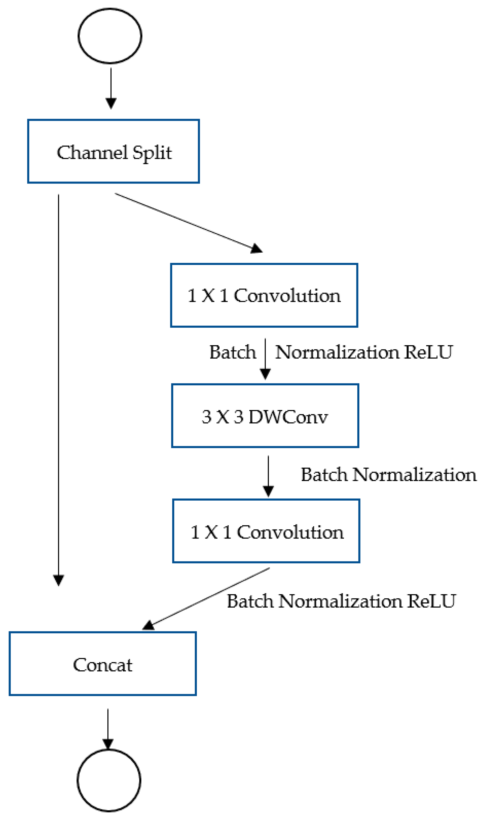
Figure 1.
Design of ShuffleNetv2.
Figure 1.
Design of ShuffleNetv2.
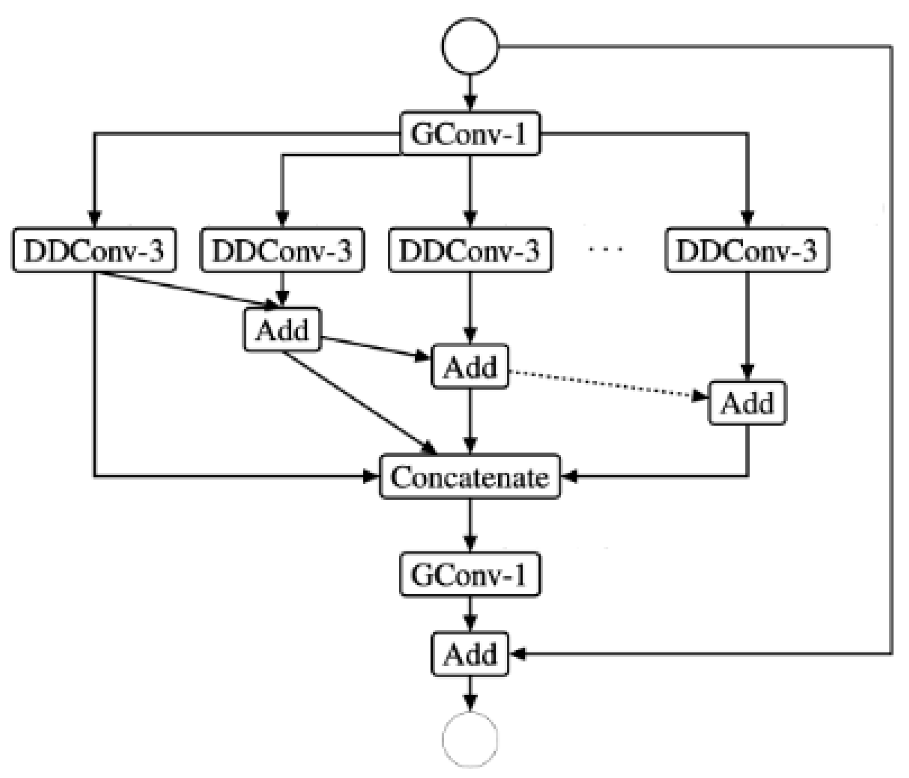
Figure 2.
EESP building block.
Figure 2.
EESP building block.
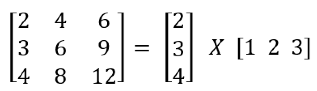
Figure 4.
Splitting a 3 × 3 kernel spatially.
Figure 4.
Splitting a 3 × 3 kernel spatially.
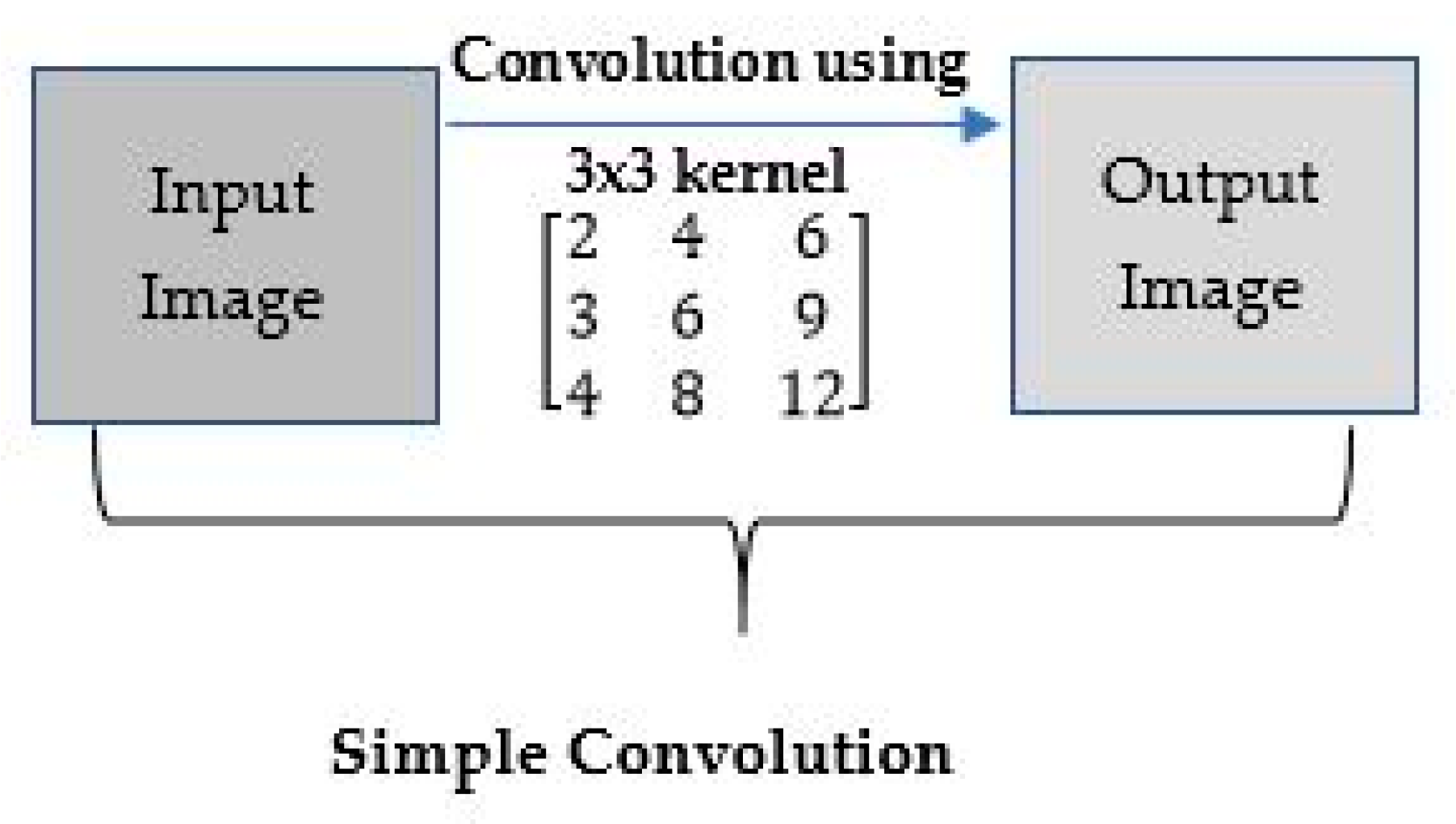
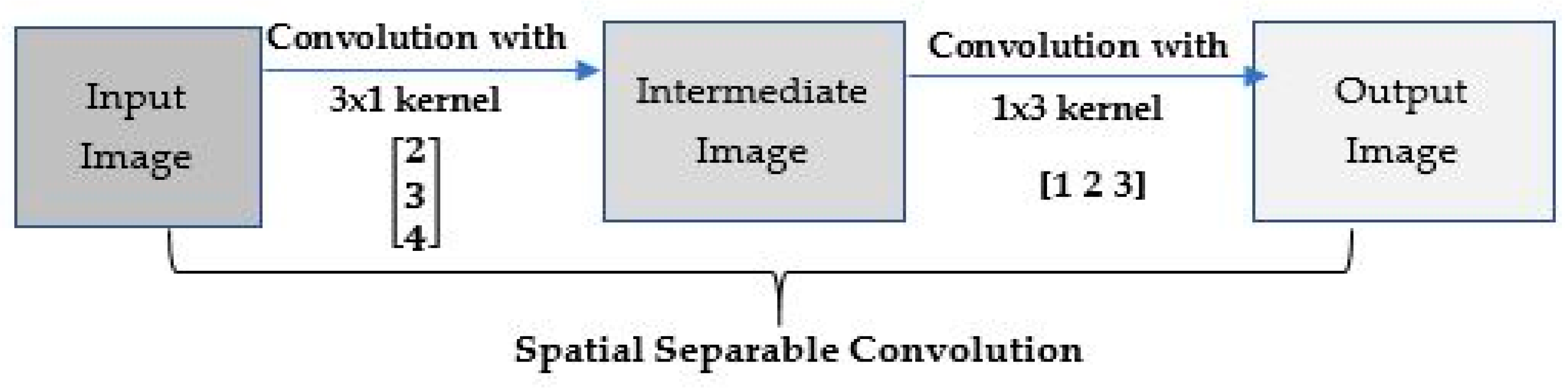
Figure 5.
Simple and Spatial Separable Convolution.
Figure 5.
Simple and Spatial Separable Convolution.
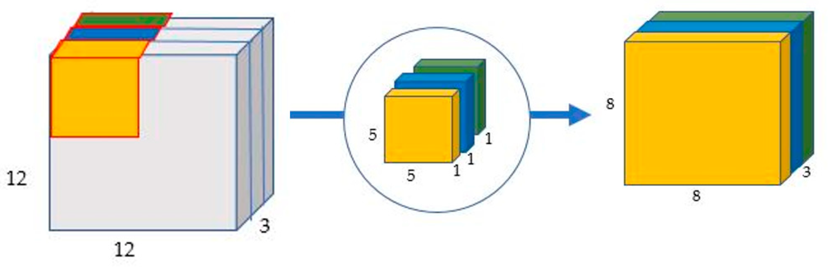
Figure 6.
Depth-wise convolution uses three kernels to produce an 8 × 8 × 1 image from a 12 × 12 × 1 image.
Figure 6.
Depth-wise convolution uses three kernels to produce an 8 × 8 × 1 image from a 12 × 12 × 1 image.
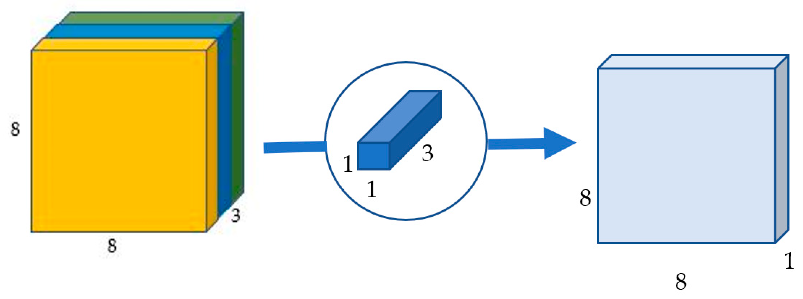
Figure 7.
Point-wise convolution transforms an image of three channels into an image of one channel.
Figure 7.
Point-wise convolution transforms an image of three channels into an image of one channel.
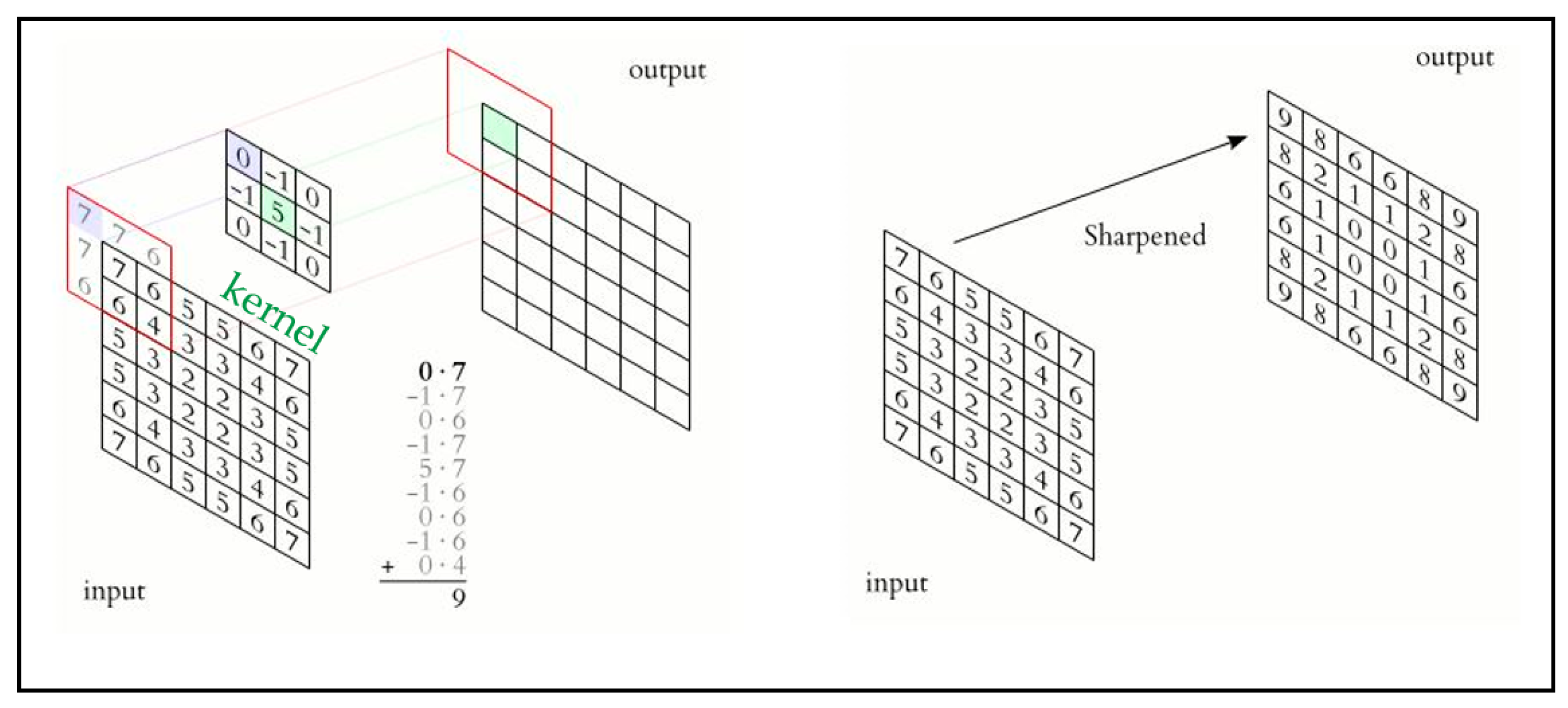
Figure 8.
Example of convolution using a kernel.
Figure 8.
Example of convolution using a kernel.
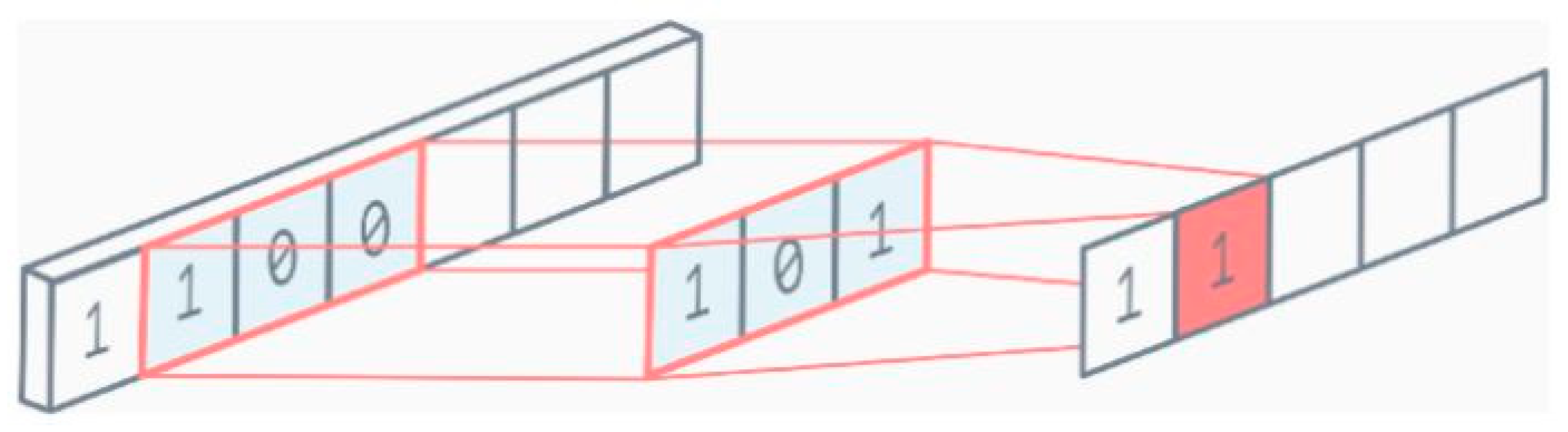
Figure 9.
1D convolution.
Figure 9.
1D convolution.
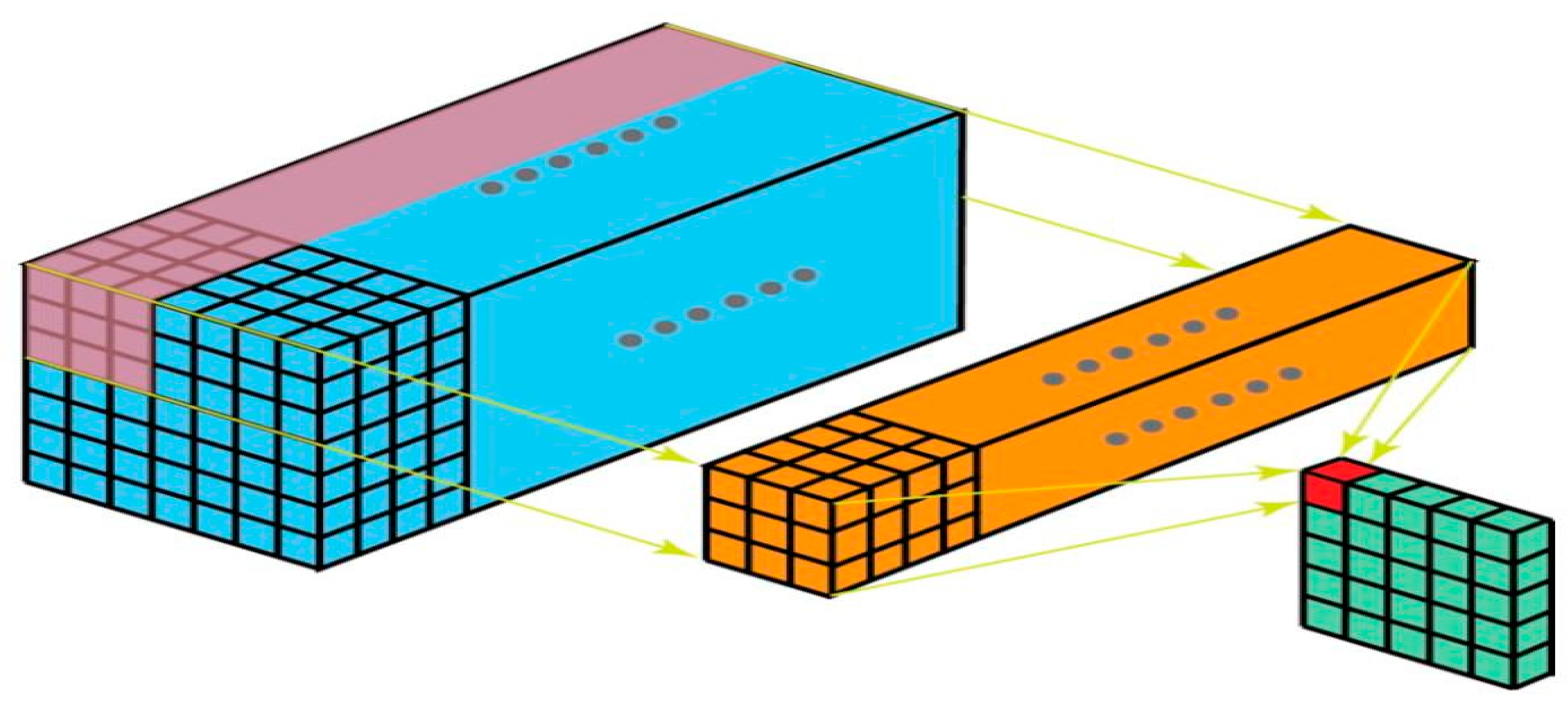
Figure 10.
2D convolution.
Figure 10.
2D convolution.
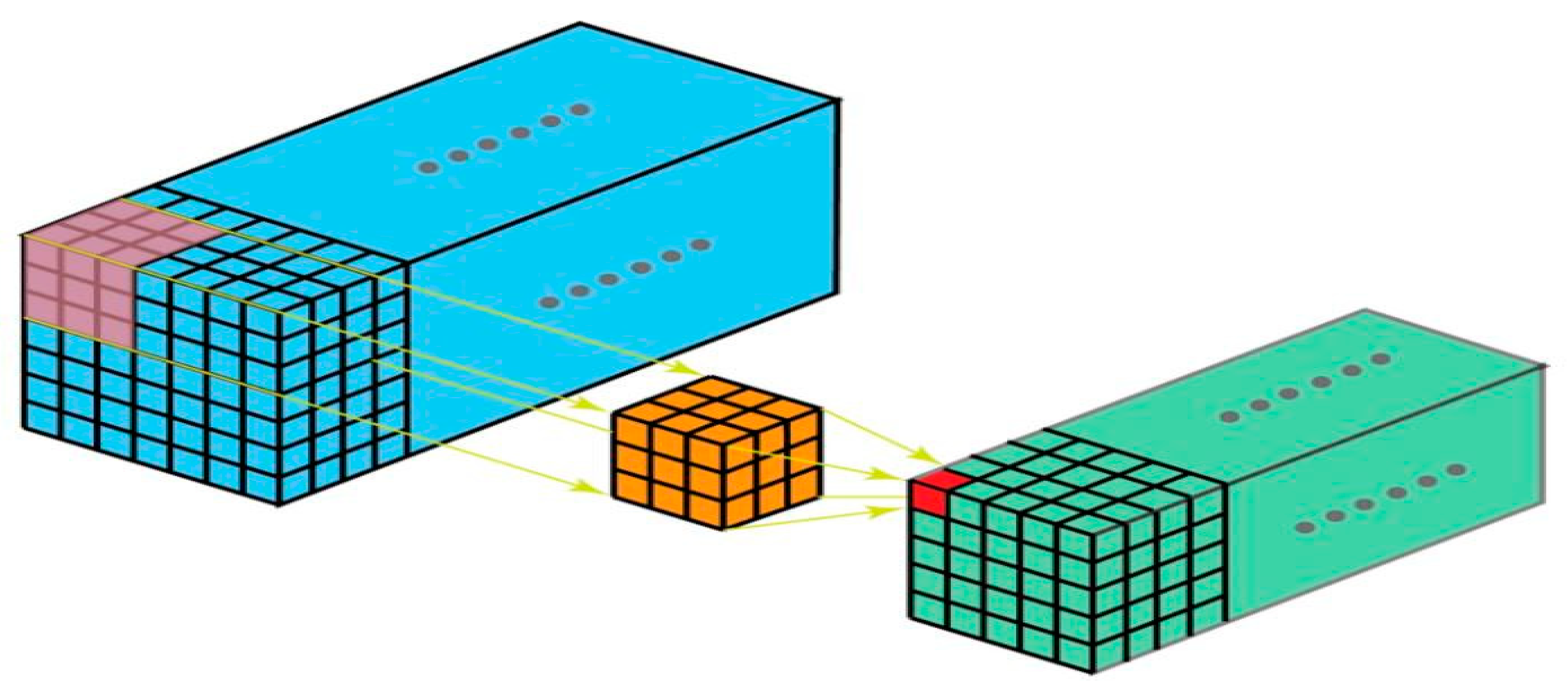
Figure 11.
3D convolution.
Figure 11.
3D convolution.
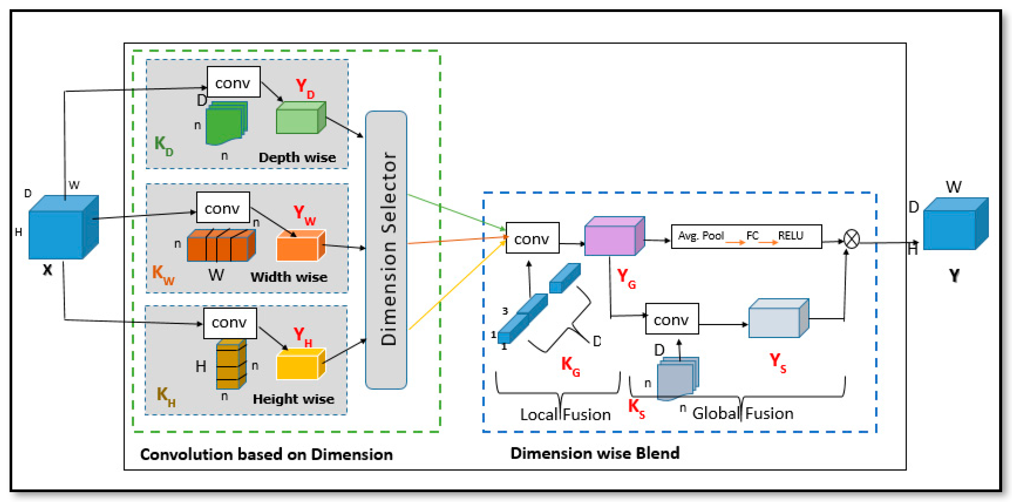
Figure 12.
DBGC architecture.
Figure 12.
DBGC architecture.
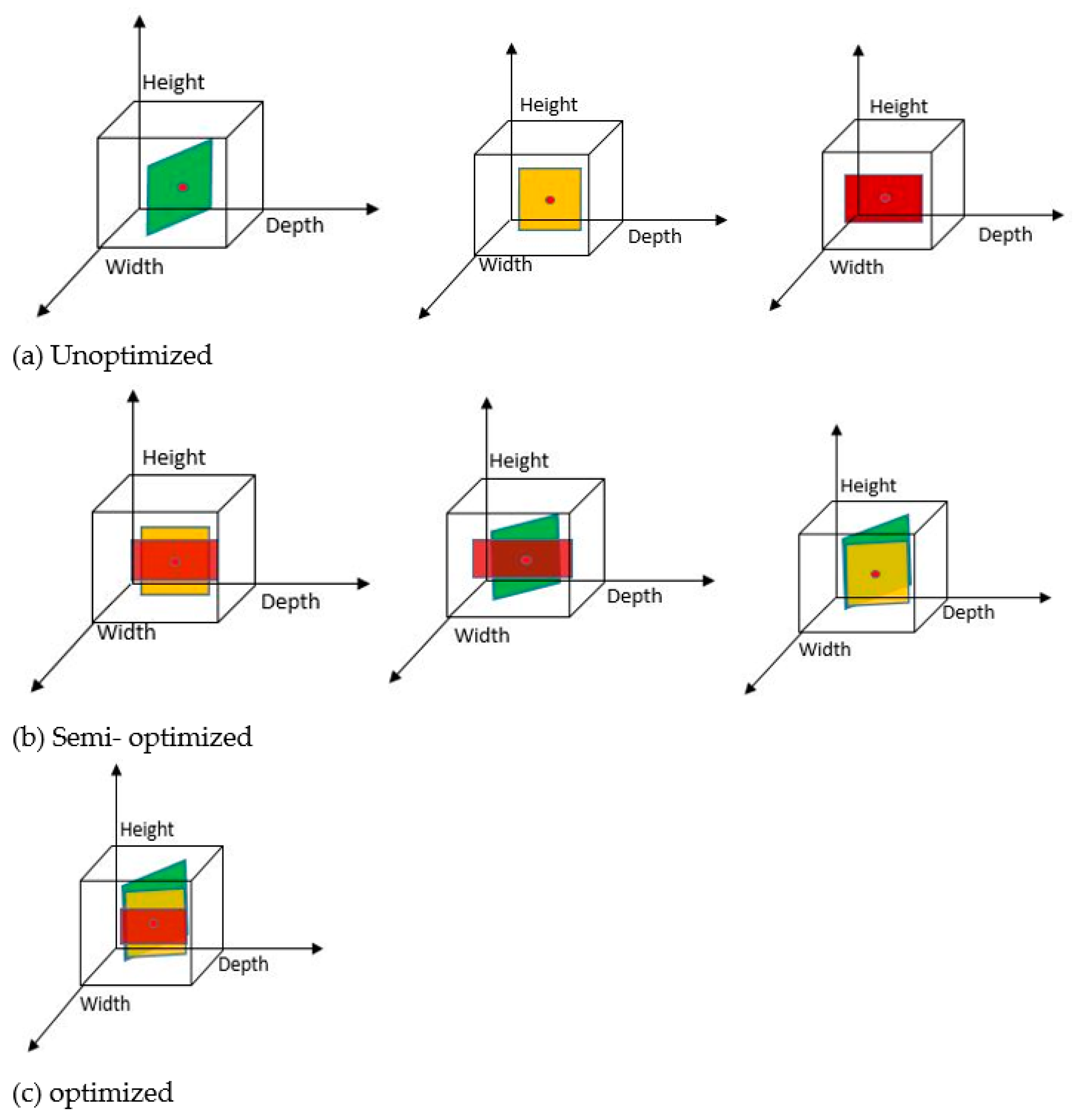
Figure 13.
Implementation of Convolution based on Dimension (ConvDim): in (a), each kernel is applied to a pixel (represented by a small dot) independently; in (b), any two kernels are (height-width, height-depth, and width-depth) applied to a pixel simultaneously by allowing information to be combined using tensors; finally in (c), all kernels are applied to a pixel simultaneously, allowing information to be aggregated from the tensor efficiently. Convolutional kernels are highlighted in color (depth-wise, width-wise, and height-wise).
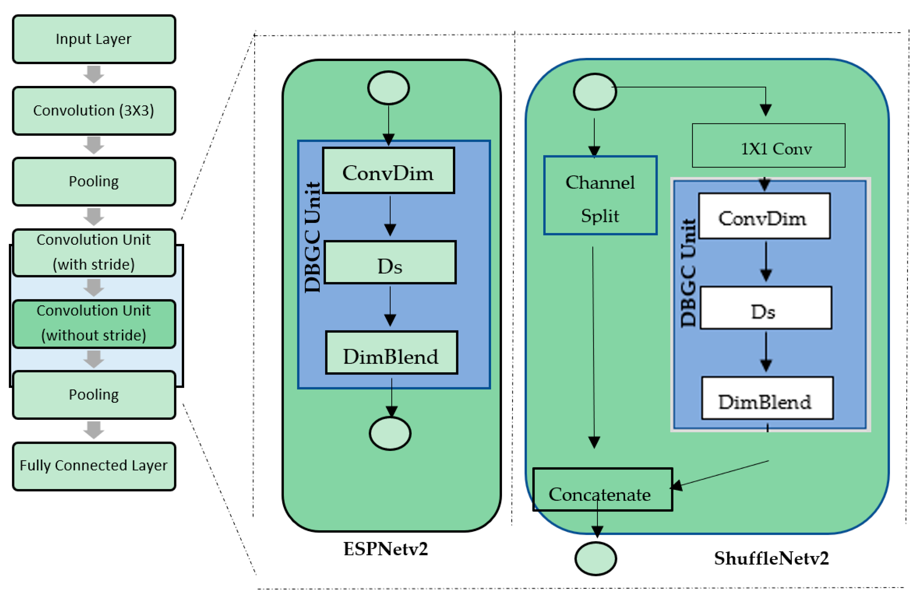
Figure 14.
The DBGC unit in different architecture (ESPNetv2 and ShuffleNetv2) designs.
Figure 14.
The DBGC unit in different architecture (ESPNetv2 and ShuffleNetv2) designs.
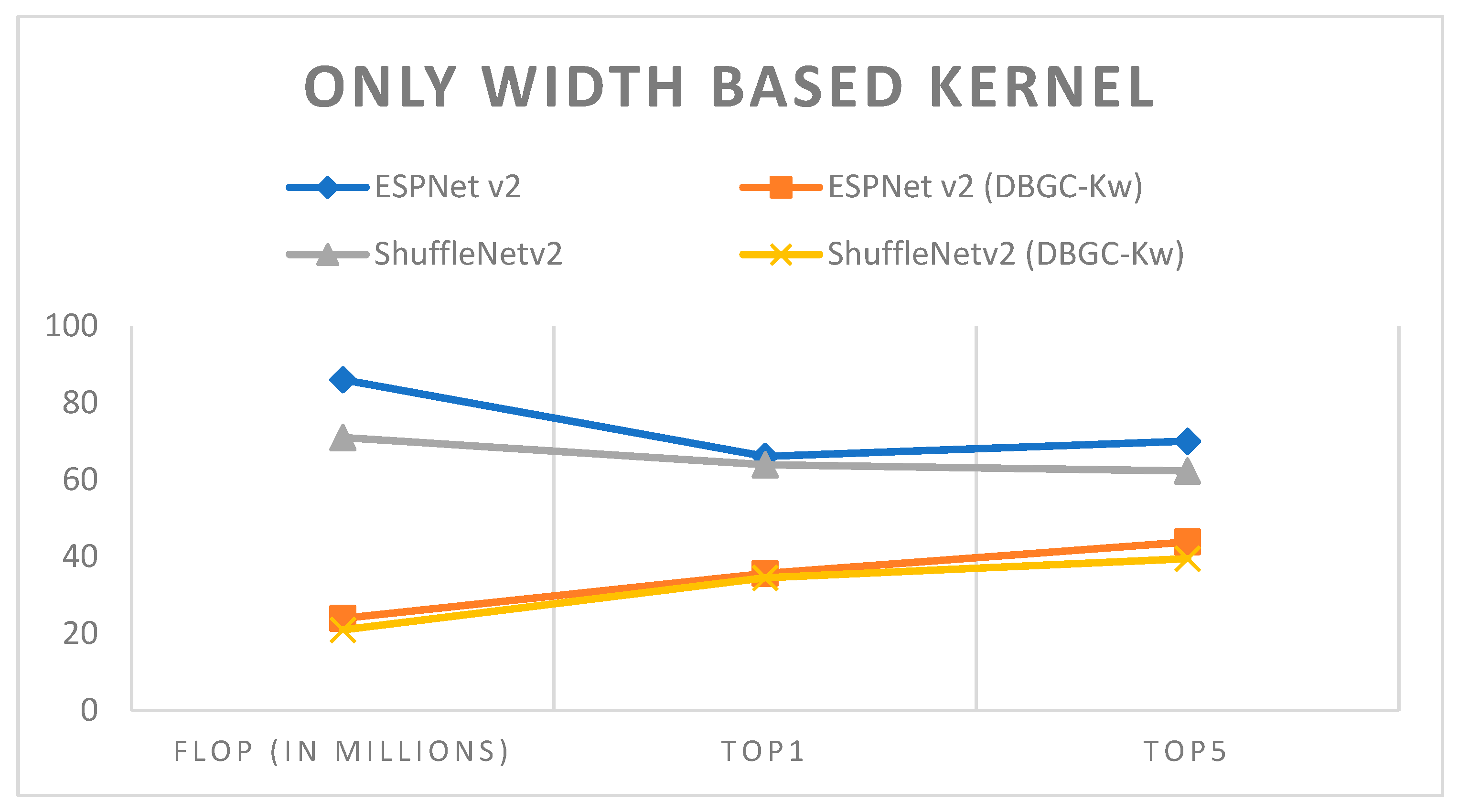
Figure 15.
Only width-based kernel.
Figure 15.
Only width-based kernel.
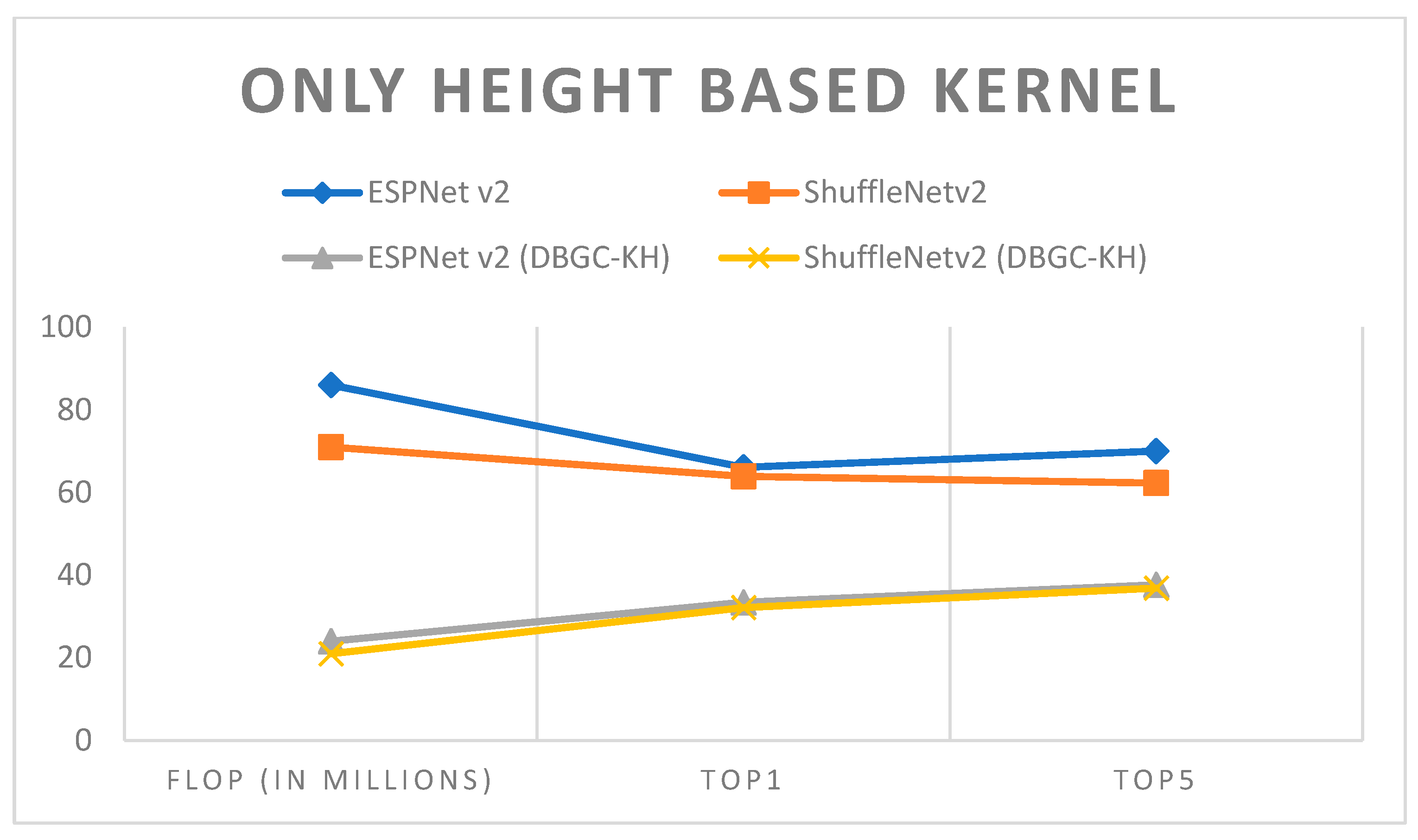
Figure 16.
Only height-based kernel.
Figure 16.
Only height-based kernel.
Figure 17.
Only depth-based kernel.
Figure 17.
Only depth-based kernel.
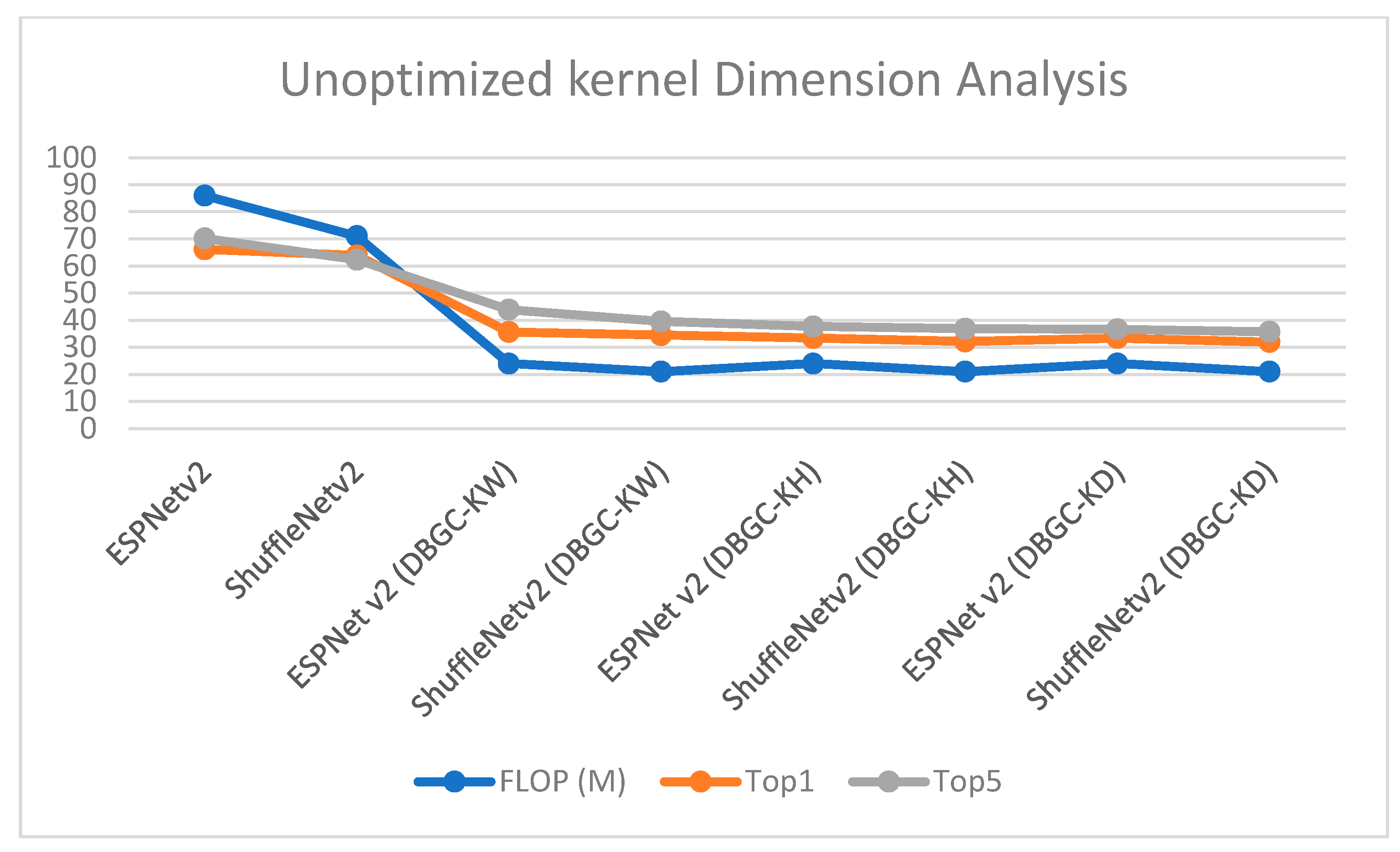
Figure 18.
Analysis of unoptimized kernel dimensions.
Figure 18.
Analysis of unoptimized kernel dimensions.
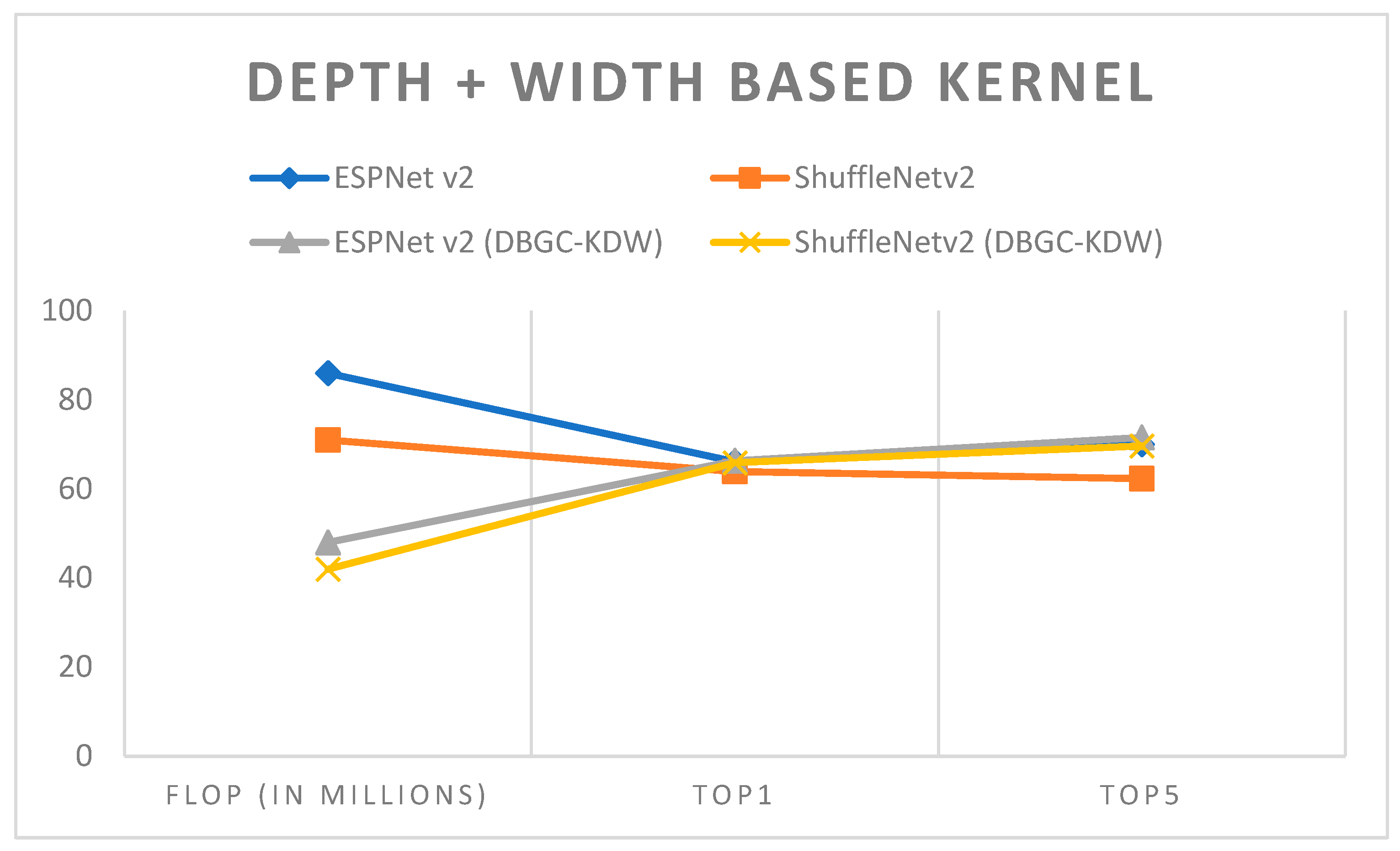
Figure 19.
Depth + width-based kernel.
Figure 19.
Depth + width-based kernel.
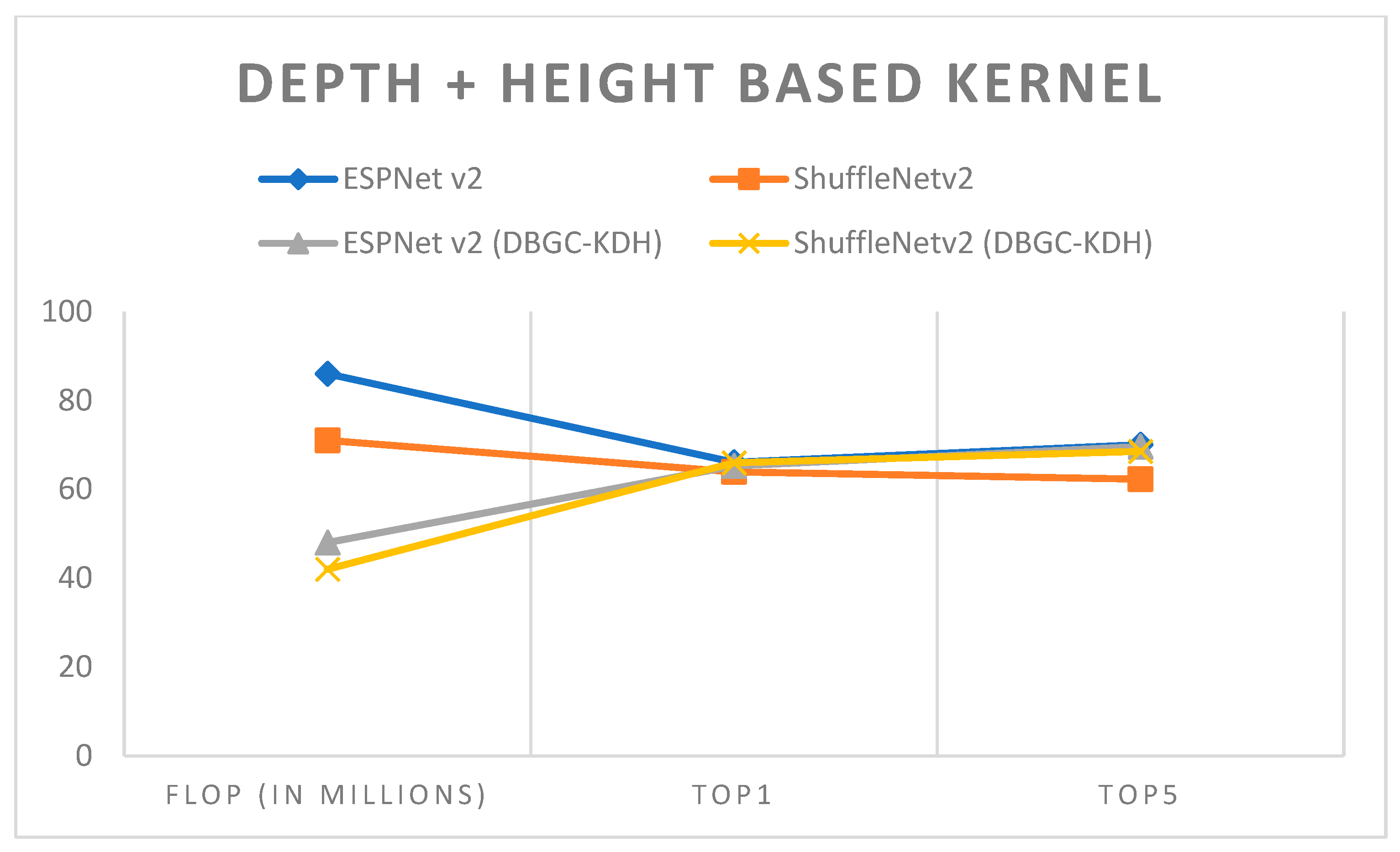
Figure 20.
Depth + height-based kernel.
Figure 20.
Depth + height-based kernel.
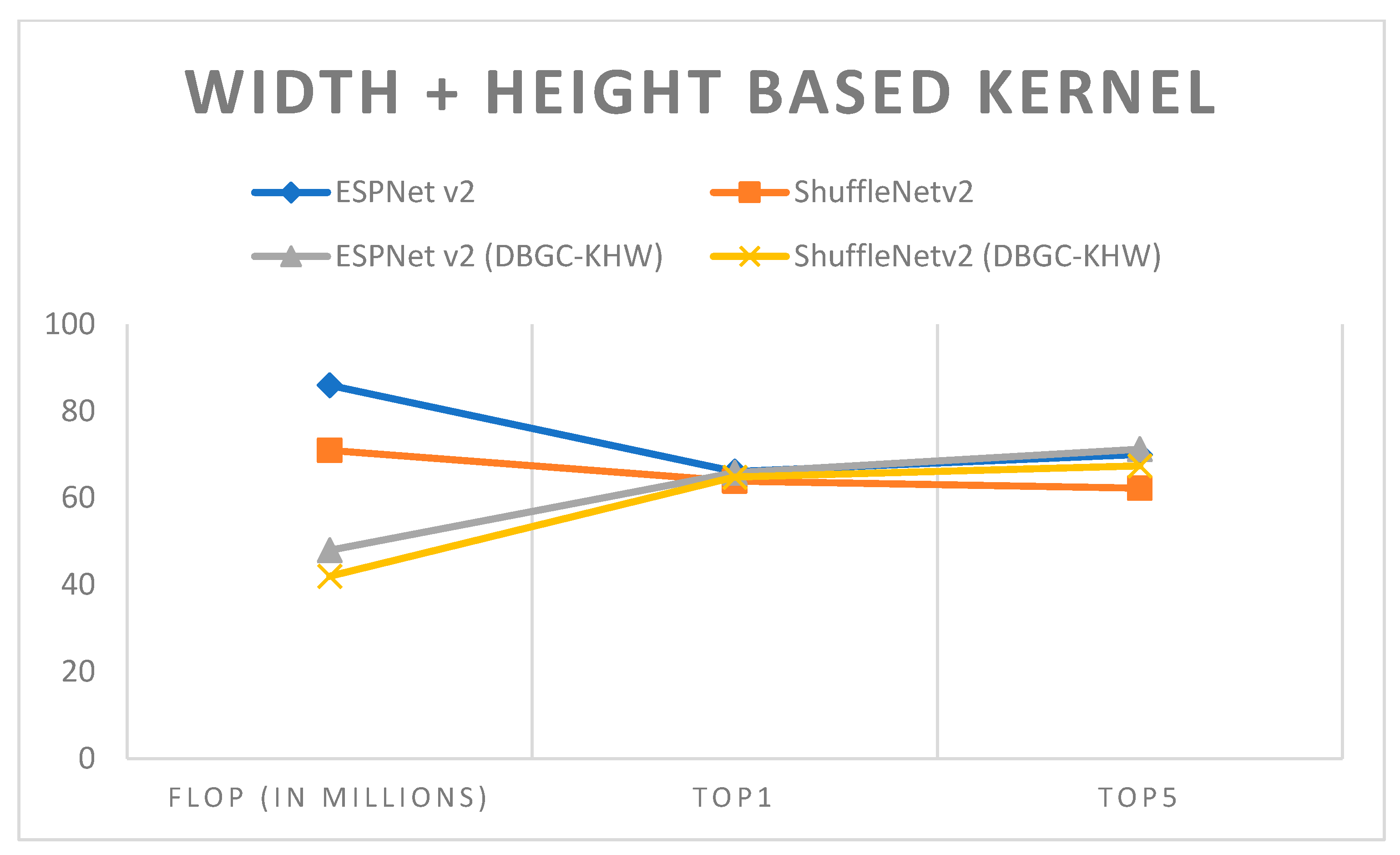
Figure 21.
Height + width-based kernel.
Figure 21.
Height + width-based kernel.
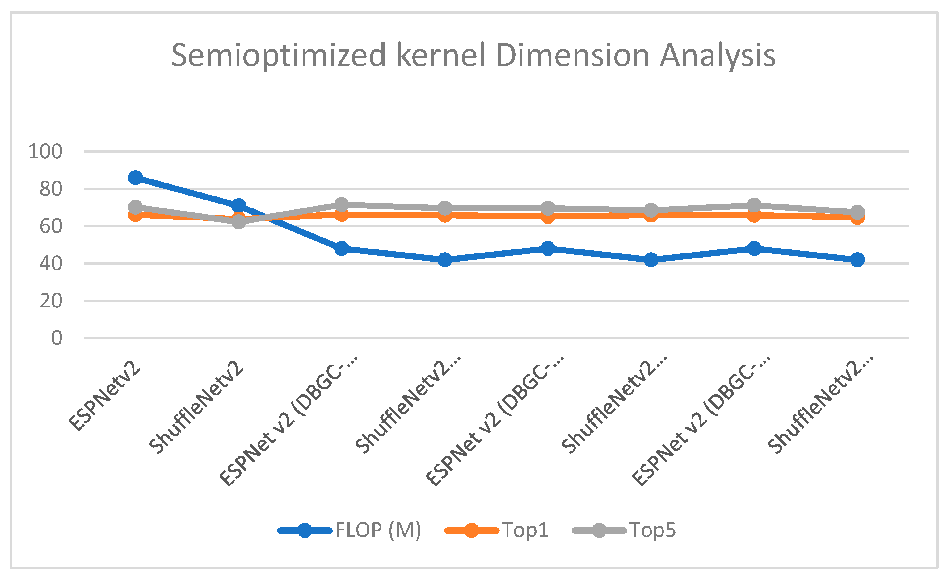
Figure 22.
Semi-optimized kernel dimension.
Figure 22.
Semi-optimized kernel dimension.
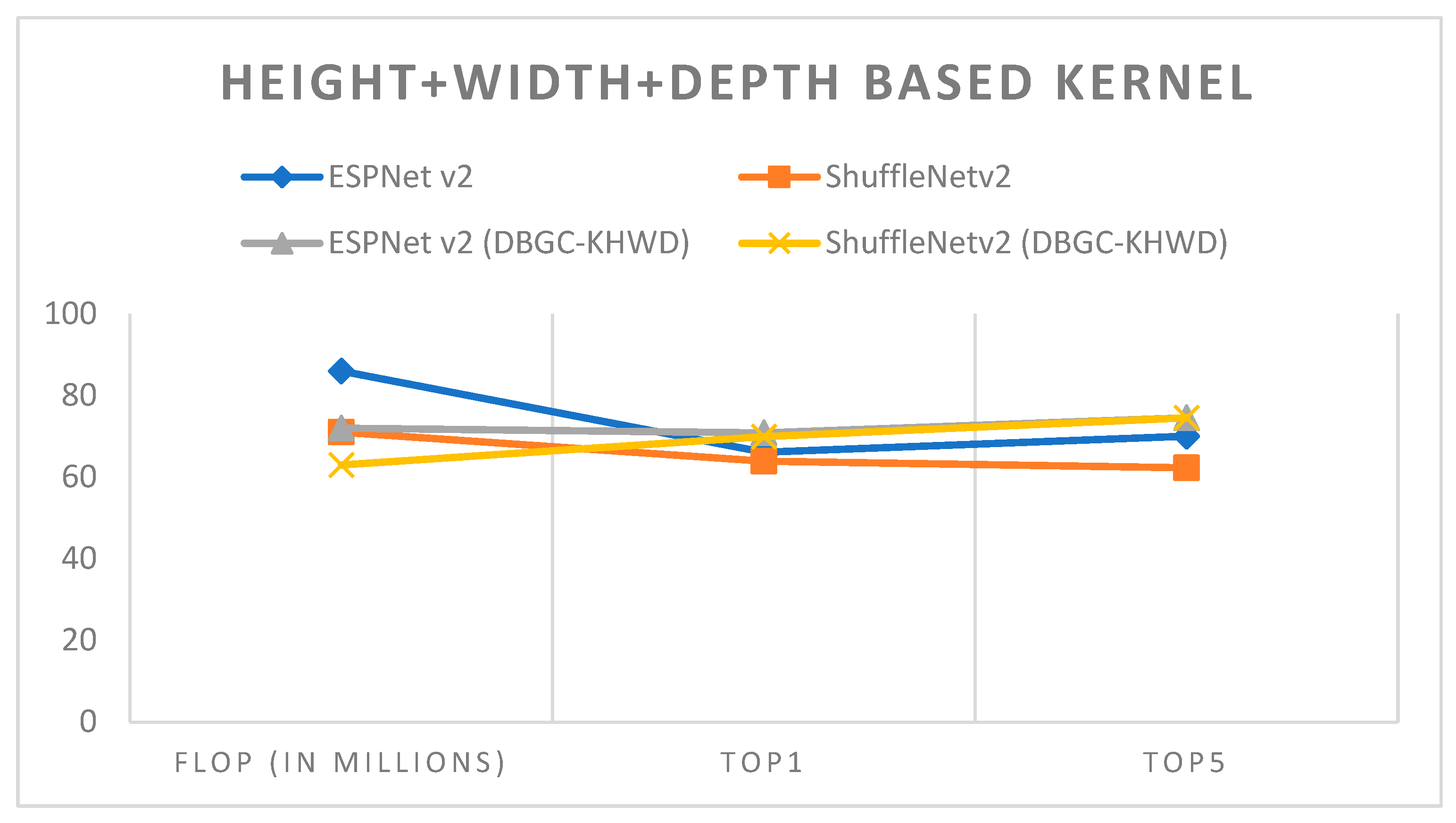
Figure 23.
Height + width + depth-based kernel.
Figure 23.
Height + width + depth-based kernel.
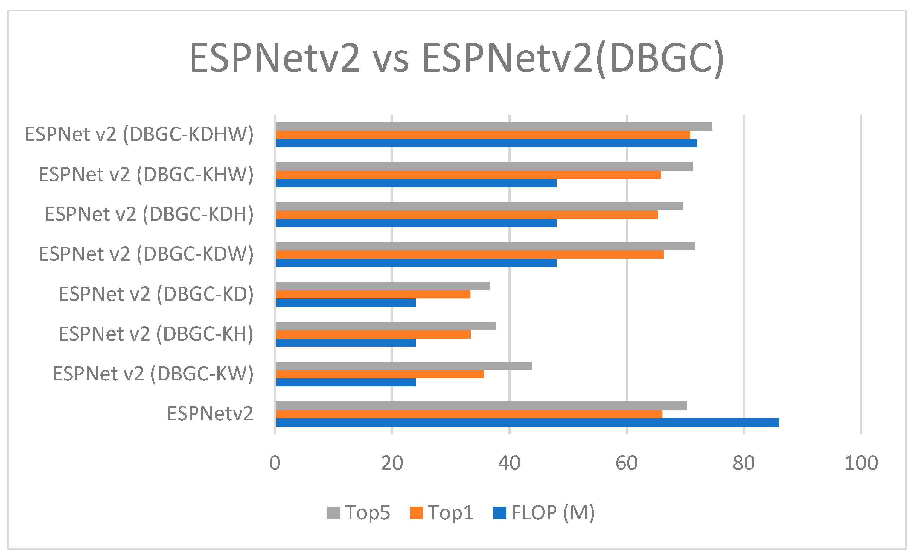
Figure 24.
ESPNetv2 versus ESPNetv2 (DBGC).
Figure 24.
ESPNetv2 versus ESPNetv2 (DBGC).
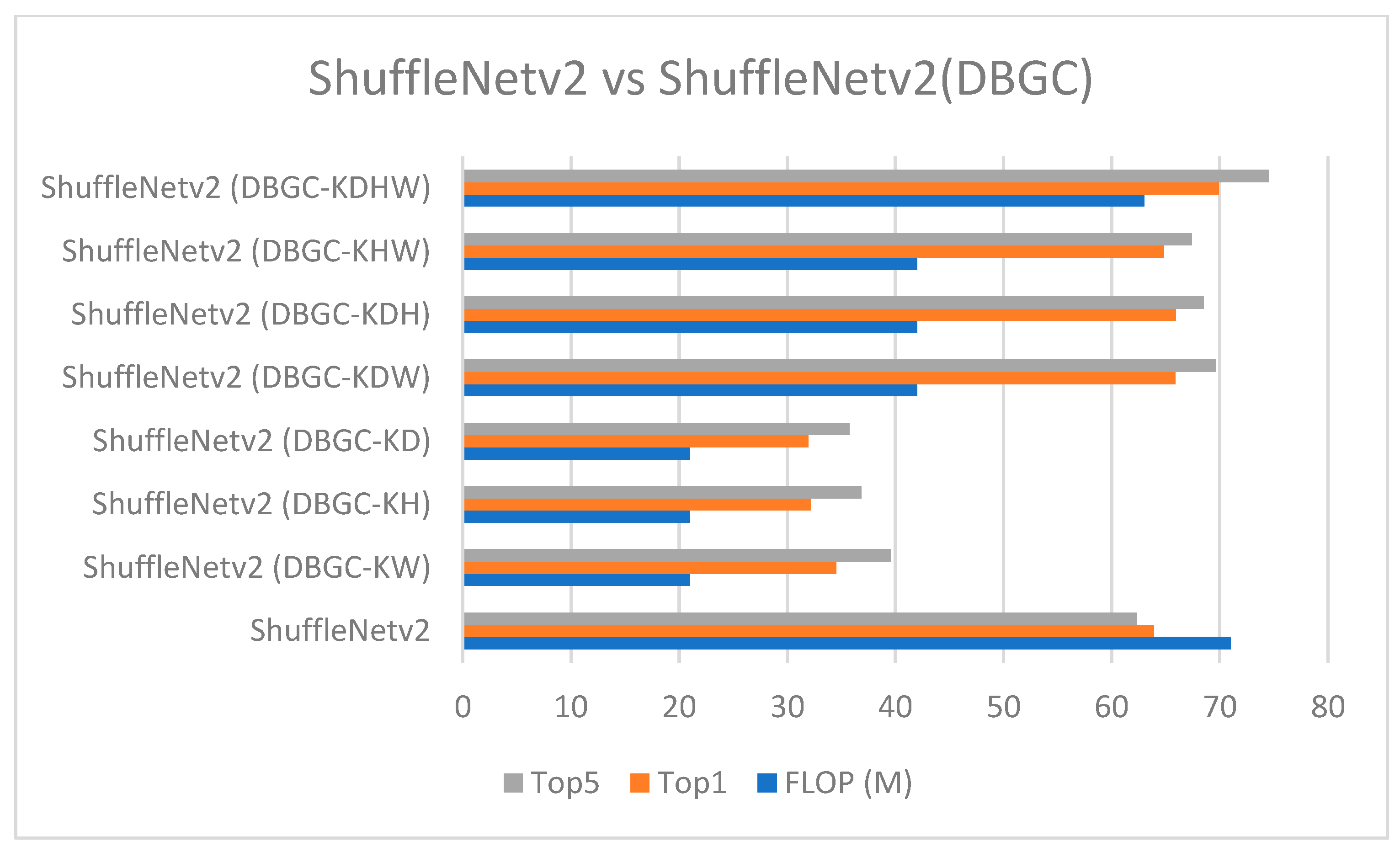
Figure 25.
ShuffleNetv2 versus ShuffleNetv2 (DBGC).
Figure 25.
ShuffleNetv2 versus ShuffleNetv2 (DBGC).
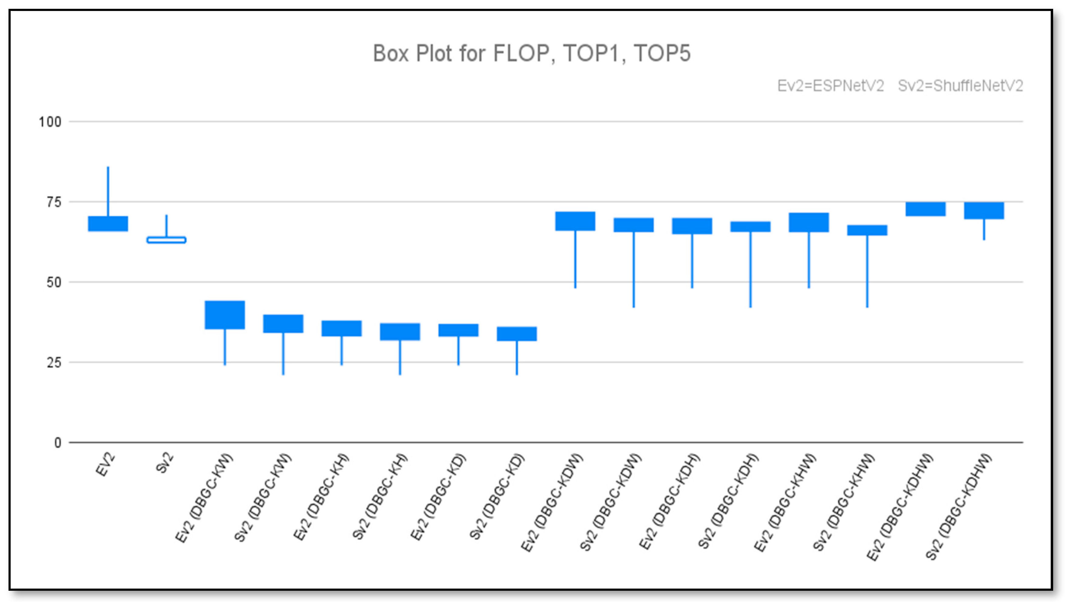
Figure 26.
Box plot to show unoptimized, semi-optimized, and optimized kernel performances for ESPNetv2 versus ESPNetV2 (DBGC) and ShuffleNetv2 versus ShuffleNetV2 (DBGC).
Figure 26.
Box plot to show unoptimized, semi-optimized, and optimized kernel performances for ESPNetv2 versus ESPNetV2 (DBGC) and ShuffleNetv2 versus ShuffleNetV2 (DBGC).
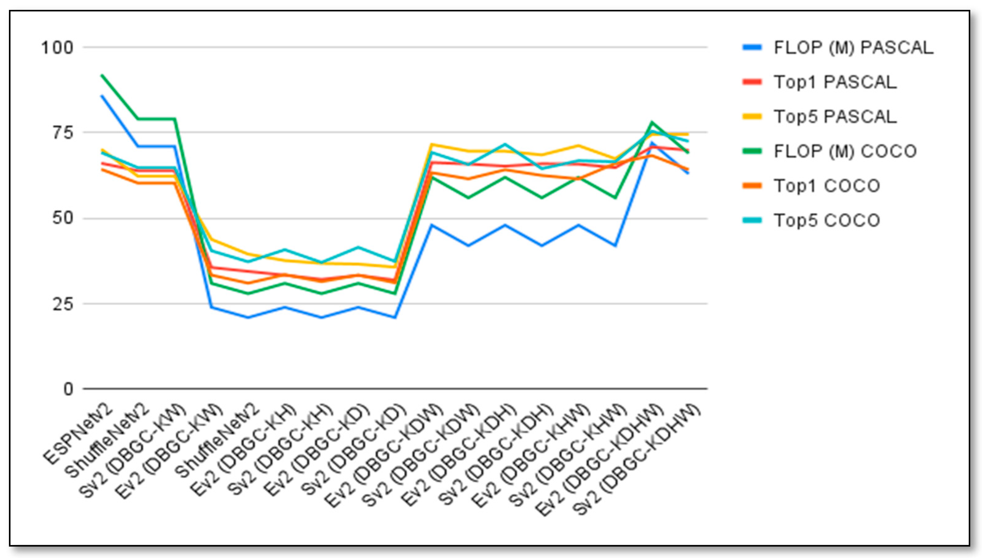
Figure 27.
Graph to visualize the performances of unoptimized, semi-optimized, and optimized kernels for ESPNetv2 versus ESPNetV2 (DBGC), and ShuffleNetv2 versus ShuffleNetV2 (DBGC) using the PASCAL and COCO datasets.
Figure 27.
Graph to visualize the performances of unoptimized, semi-optimized, and optimized kernels for ESPNetv2 versus ESPNetV2 (DBGC), and ShuffleNetv2 versus ShuffleNetV2 (DBGC) using the PASCAL and COCO datasets.
Table 2.
Equations to calculate FLOPs of each CNN layer.
Table 2.
Equations to calculate FLOPs of each CNN layer.
| Sr. No | Layer | The Equation to Calculate FLOPs |
|---|
| 1 | Convolution Layer | 2 × No. of Kernel × Kernel’s Shape × Output Shape × Repeat Count (if available) |
| 2 | Pooling Layer
(Without stride) | Height × Width × Depth of an input Image |
| 3 | Pooling Layer
(With stride) | (Height/Stride) × Depth × (Width/Stride) of an input Image |
| 4 | Fully Connected Layer (FC Layer) | 2 × Input Size × Output Size |
Table 3.
Only width-based kernel.
Table 3.
Only width-based kernel.
| Model | Dataset | Image Size | FLOP (In Millions) | Top1 | Top5 |
|---|
| ESPNet v2 | PASCAL | 224 × 224 | 86 | 66.1 | 70.02 |
| ShuffleNetv2 | PASCAL | 224 × 224 | 71 | 63.9 | 62.30 |
| ESPNetv2(DBGC-Kw) | PASCAL | 224 × 224 | 24 | 35.64 | 43.86 |
| ShuffleNetv2 (DBGC-Kw) | PASCAL | 224 × 224 | 21 | 34.5 | 39.54 |
Table 4.
Only height-based kernel.
Table 4.
Only height-based kernel.
| Model | Dataset | Image Size | FLOP (In Millions) | Top1 | Top5 |
|---|
| ESPNet v2 | PASCAL | 224 × 224 | 86 | 66.1 | 70.02 |
| ShuffleNetv2 | PASCAL | 224 × 224 | 71 | 63.9 | 62.30 |
| ESPNetv2(DBGC-KH) | PASCAL | 224 × 224 | 24 | 33.4 | 37.66 |
| ShuffleNetv2 (DBGC-KH) | PASCAL | 224 × 224 | 21 | 32.15 | 36.84 |
Table 5.
Only depth-based kernel.
Table 5.
Only depth-based kernel.
| Model | Dataset | Image Size | FLOP (In Millions) | Top1 | Top5 |
|---|
| ESPNet v2 | PASCAL | 224 × 224 | 86 | 66.1 | 70.02 |
| ShuffleNetv2 | PASCAL | 224 × 224 | 71 | 63.9 | 62.30 |
| ESPNetv2(DBGC-KD) | PASCAL | 224 × 224 | 24 | 33.34 | 36.62 |
| ShuffleNetv2 (DBGC-KD) | PASCAL | 224 × 224 | 21 | 31.95 | 35.74 |
Table 6.
Depth + width-based kernel.
Table 6.
Depth + width-based kernel.
| Model | Dataset | Image Size | FLOP (In Millions) | Top1 | Top5 |
|---|
| ESPNet v2 | PASCAL | 224 × 224 | 86 | 66.1 | 70.02 |
| ShuffleNetv2 | PASCAL | 224 × 224 | 71 | 63.9 | 62.30 |
| ESPNetv2(DBGC-KDW) | PASCAL | 224 × 224 | 48 | 66.31 | 71.58 |
| ShuffleNetv2 (DBGC-KDW) | PASCAL | 224 × 224 | 42 | 65.88 | 69.65 |
Table 7.
Depth + height-based kernel.
Table 7.
Depth + height-based kernel.
| Model | Dataset | Image Size | FLOP (In Millions) | Top1 | Top5 |
|---|
| ESPNet v2 | PASCAL | 224 × 224 | 86 | 66.1 | 70.02 |
| ShuffleNetv2 | PASCAL | 224 × 224 | 71 | 63.9 | 62.30 |
| ESPNetv2(DBGC-KDH) | PASCAL | 224 × 224 | 48 | 65.25 | 69.63 |
| ShuffleNetv2 (DBGC-KDH) | PASCAL | 224 × 224 | 42 | 65.95 | 68.53 |
Table 8.
Height + width-based kernel.
Table 8.
Height + width-based kernel.
| Model | Dataset | Image Size | FLOP (In Millions) | Top1 | Top5 |
|---|
| ESPNet v2 | PASCAL | 224 × 224 | 86 | 66.1 | 70.02 |
| ShuffleNetv2 | PASCAL | 224 × 224 | 71 | 63.9 | 62.30 |
| ESPNetv2(DBGC-KHW) | PASCAL | 224 × 224 | 48 | 65.85 | 71.25 |
| ShuffleNetv2(DBGCKHW) | PASCAL | 224 × 224 | 42 | 64.82 | 67.43 |
Table 9.
Height + width + depth-based kernel.
Table 9.
Height + width + depth-based kernel.
| Model | Dataset | Image Size | FLOP (In Millions) | Top1 | Top5 |
|---|
| ESPNet v2 | PASCAL | 224 × 224 | 86 | 66.1 | 70.02 |
| ShuffleNetv2 | PASCAL | 224 × 224 | 71 | 63.9 | 62.30 |
| ESPNetv2(DBGC-KHWD) | PASCAL | 224 × 224 | 72 | 70.83 | 74.56 |
| ShuffleNetv2 (DBGC-KHWD) | PASCAL | 224 × 224 | 63 | 69.92 | 74.53 |
Table 10.
Unoptimized, semi-optimized, and optimized kernel performances for ESPNetv2 versus ESPNetV2 (DBGC) and ShuffleNetv2 versus ShuffleNetV2 (DBGC) for the PASCAL and COCO datasets.
Table 10.
Unoptimized, semi-optimized, and optimized kernel performances for ESPNetv2 versus ESPNetV2 (DBGC) and ShuffleNetv2 versus ShuffleNetV2 (DBGC) for the PASCAL and COCO datasets.
| | Dataset | ESPNetv2 (Ev2) | ShufleNetv2 (Sv2) | Ev2(DBGC-KW) | Sv2 (DBGC-KW) | Ev2(DBGC-KH) | Sv2(DBGC-KH) | Ev2(DBGC-KD) | Sv2(DBGC-KD) | Ev2(DBGC-KDW) | Sv2(DBGC-KDW) | Ev2(DBGC-KDH) | Sv2(DBGC-KDH) | Ev2(DBGC-KHW) | Sv2(DBGC-KHW) | Ev2(DBGC-KDHW) | Sv2(DBGC-KDHW) |
|---|
| FLOP (M) | PASCAL | 86 | 71 | 24 | 21 | 24 | 21 | 24 | 21 | 48 | 42 | 48 | 42 | 48 | 42 | 72 | 63 |
| Top1 | 66.1 | 63.9 | 35.64 | 34.5 | 33.4 | 32.15 | 33.34 | 31.95 | 66.31 | 65.88 | 65.25 | 65.95 | 65.85 | 64.82 | 70.83 | 69.92 |
| Top5 | 70.2 | 62.3 | 43.86 | 39.54 | 37.66 | 36.84 | 36.62 | 35.74 | 71.58 | 69.65 | 69.63 | 68.53 | 71.25 | 67.43 | 74.56 | 74.53 |
| FLOP (M) | COCO | 92 | 79 | 31 | 28 | 31 | 28 | 31 | 28 | 62 | 56 | 62 | 56 | 62 | 56 | 78 | 69 |
| Top1 | 64.34 | 60.3 | 33.41 | 31.05 | 33.54 | 31.5 | 33.42 | 31.17 | 63.33 | 61.54 | 64.21 | 62.53 | 61.53 | 66.05 | 68.34 | 64.23 |
| Top5 | 69.23 | 64.8 | 40.53 | 37.31 | 40.83 | 37.11 | 41.53 | 37.41 | 69.25 | 65.72 | 71.63 | 64.53 | 66.85 | 66.55 | 75.46 | 72.5 |


 ,
, 


