
Performance of Linear Mixed Models to Assess the Effect of Sustained Loading and Variable Temperature on Concrete Beams Strengthened with NSM-FRP


Abstract
:1. Introduction
2. EMI Method
3. Experimental Programme
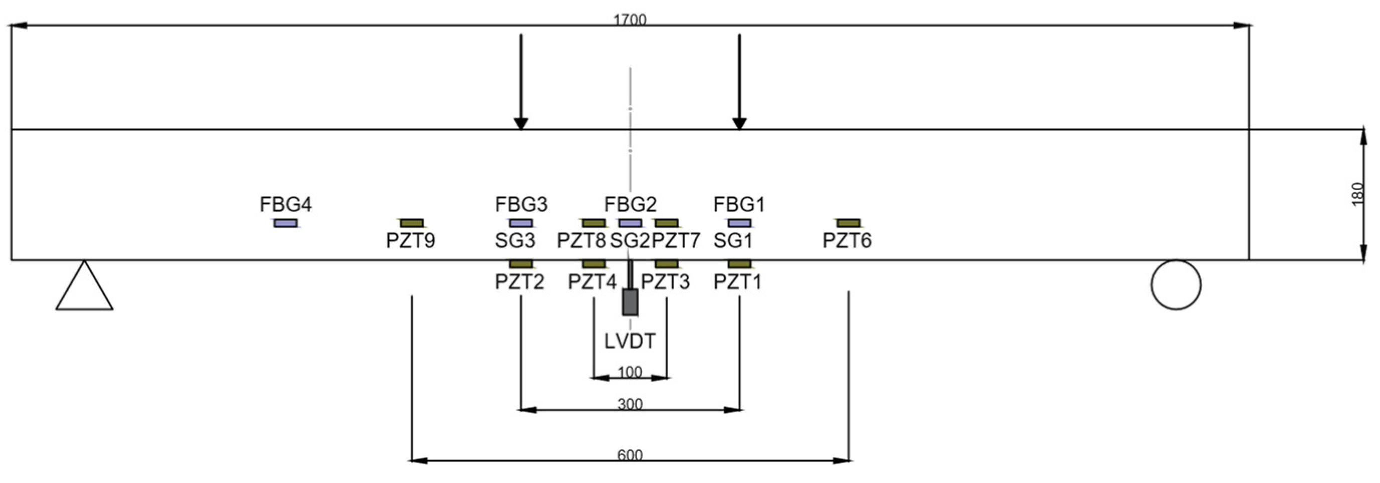
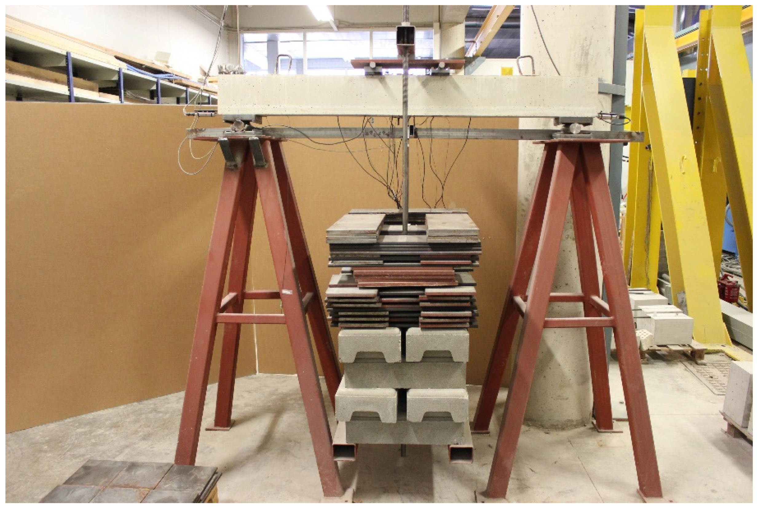
3.1. Test Set-Up
3.2. Loading Procedure
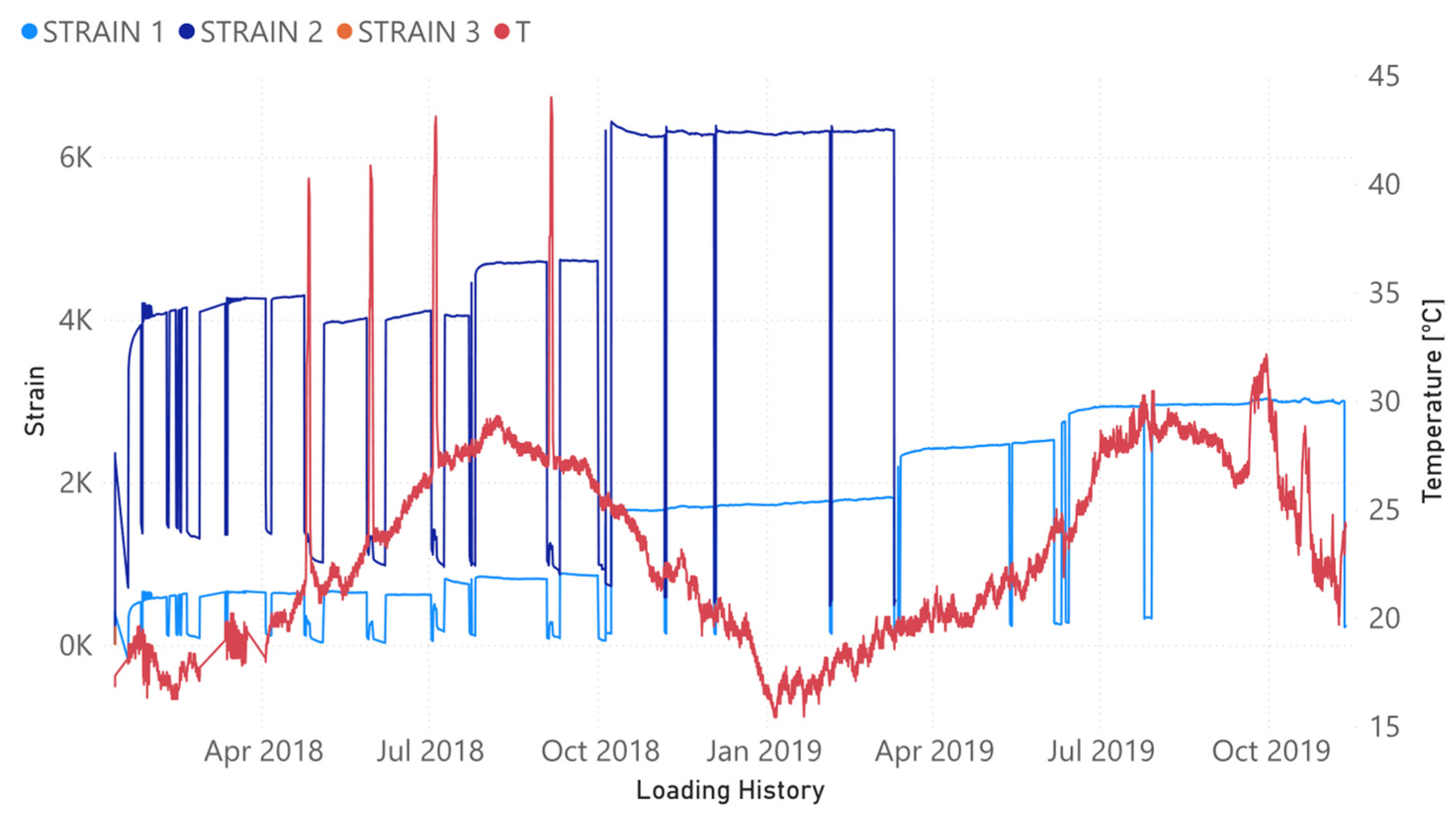
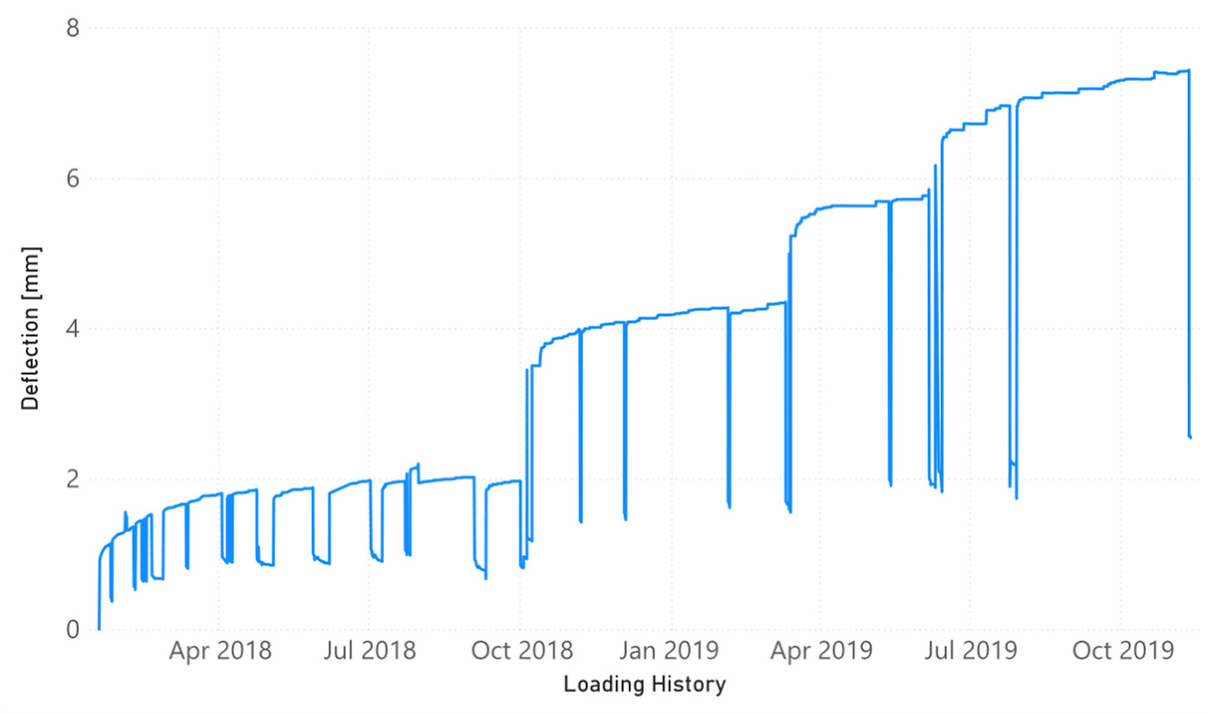
3.3. Results
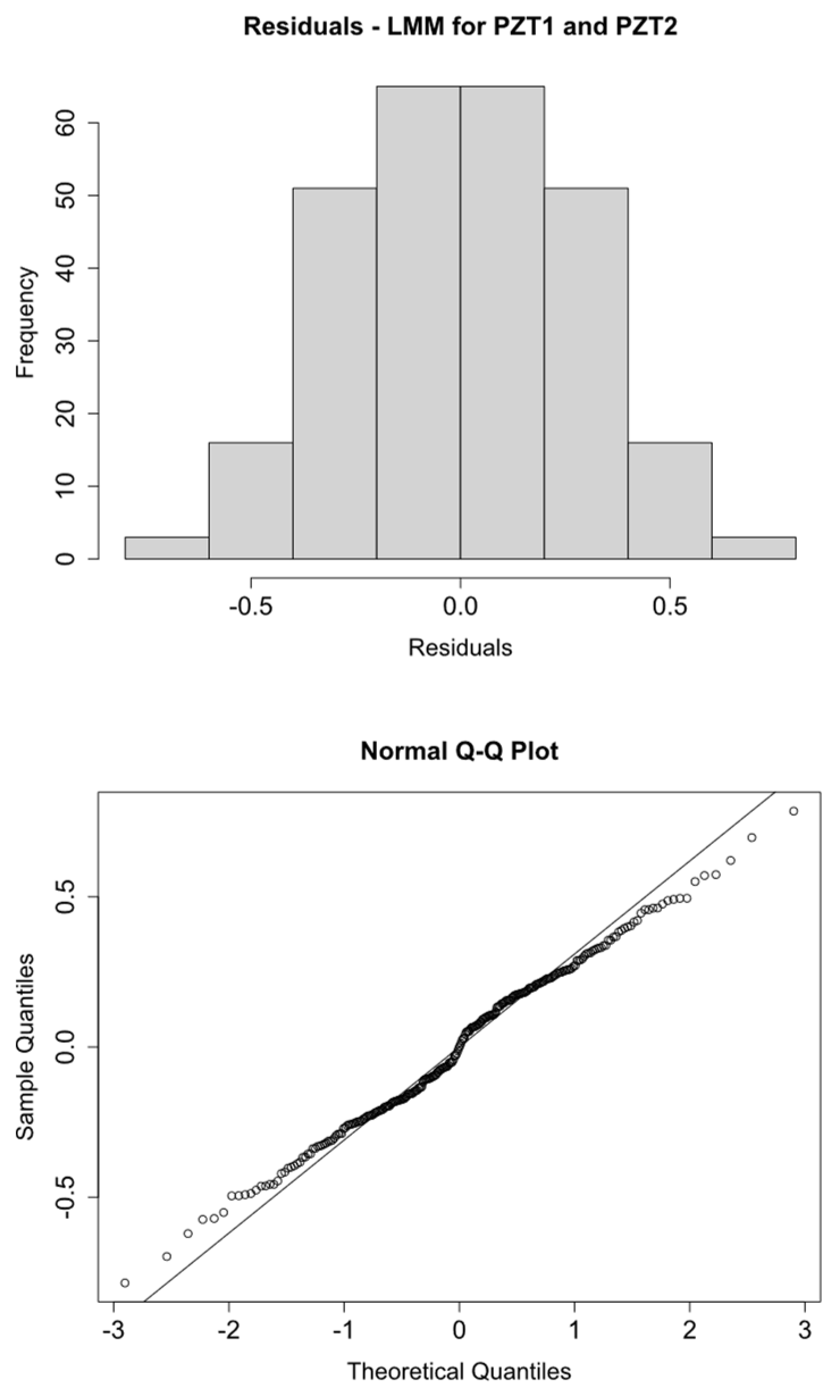
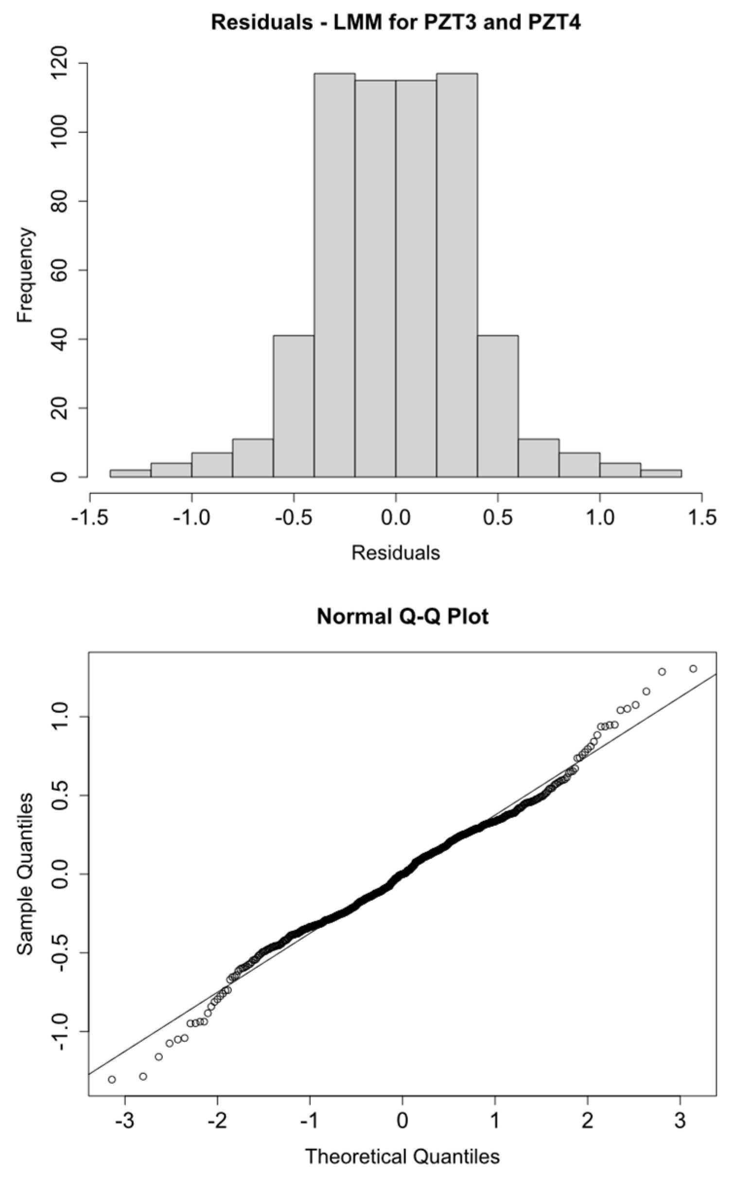
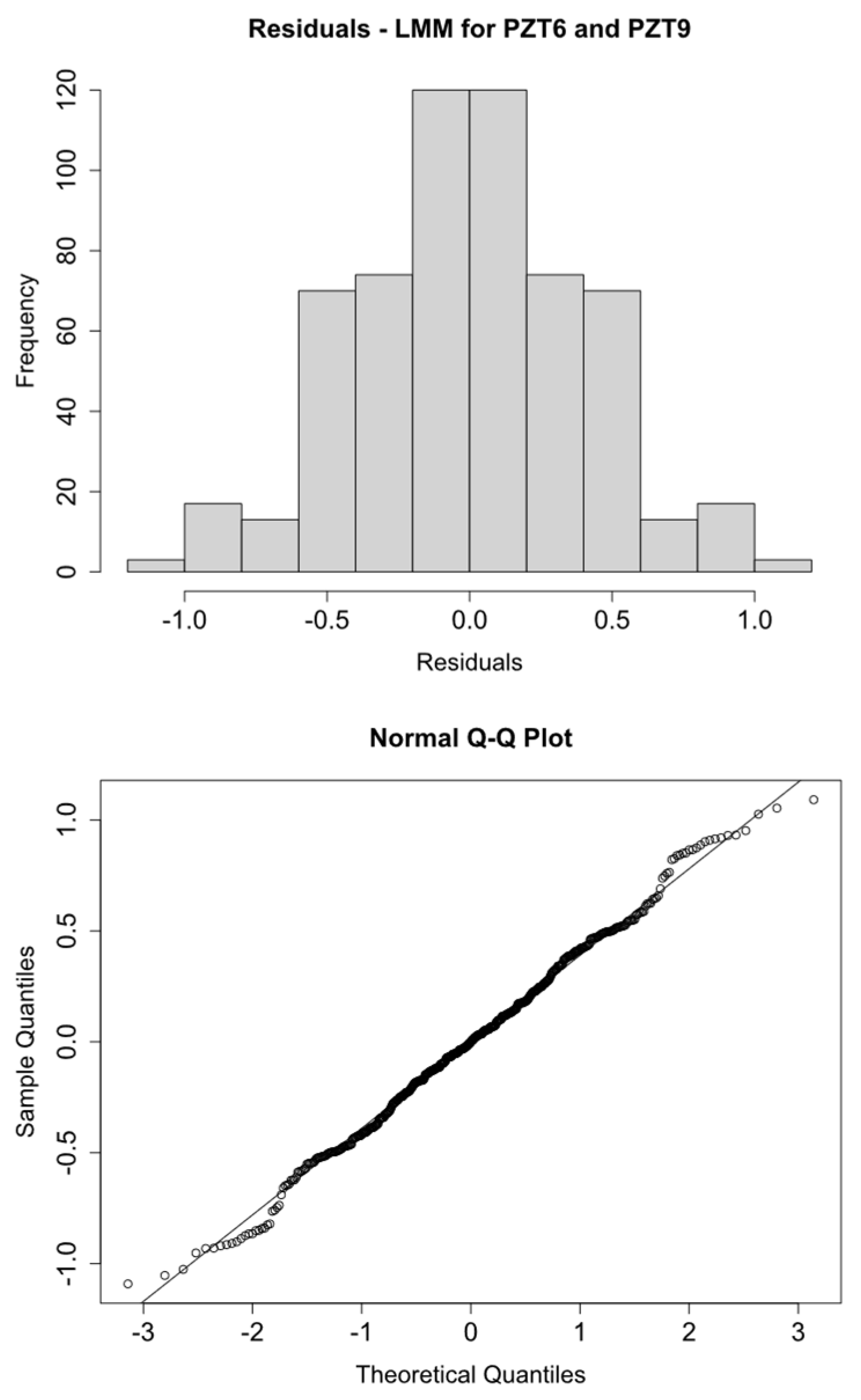
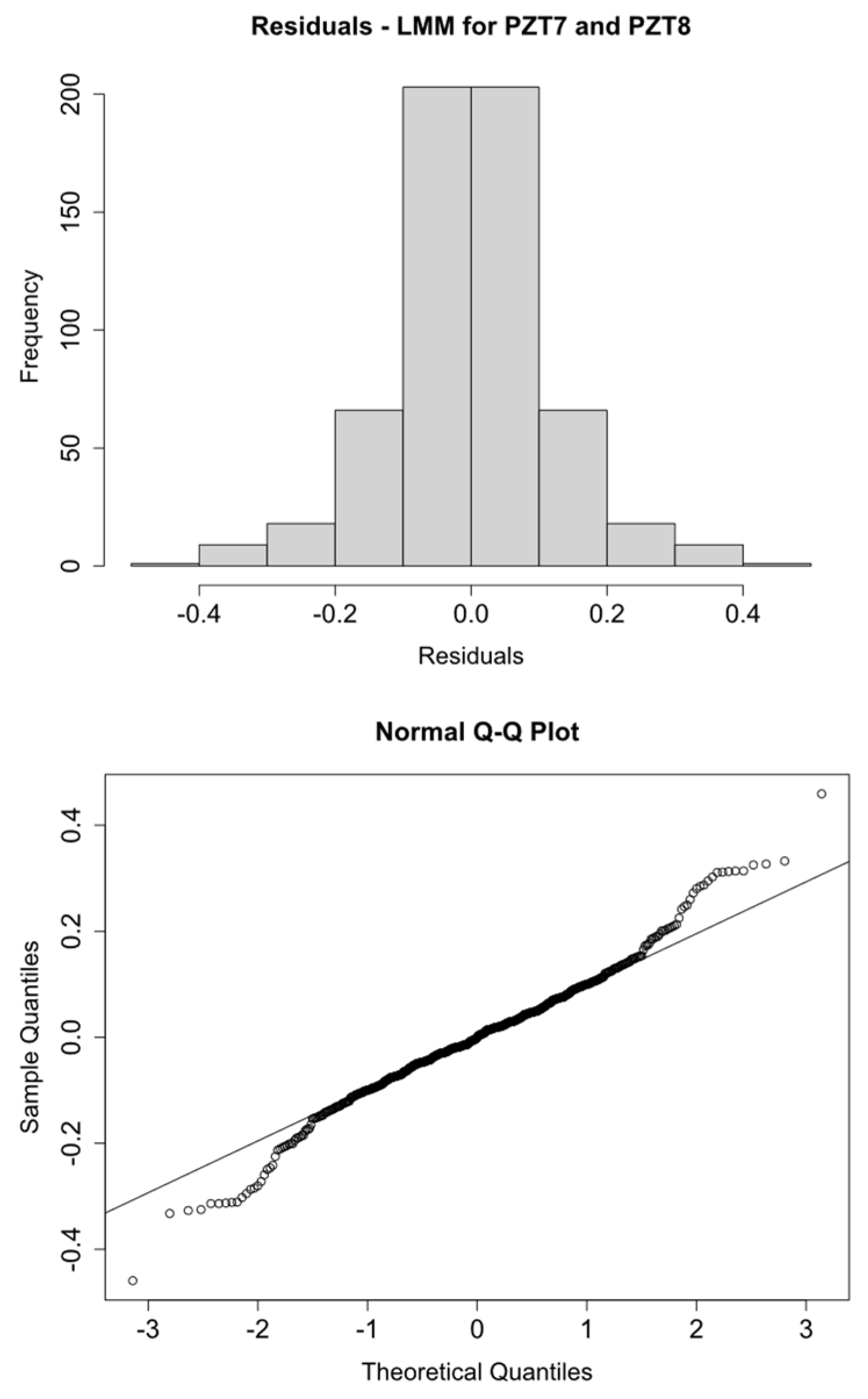
4. LMM Analysis
4.1. Linear Mixed Model
4.2. Preliminary Analysis
4.3. Statistical Analysis
- (a)
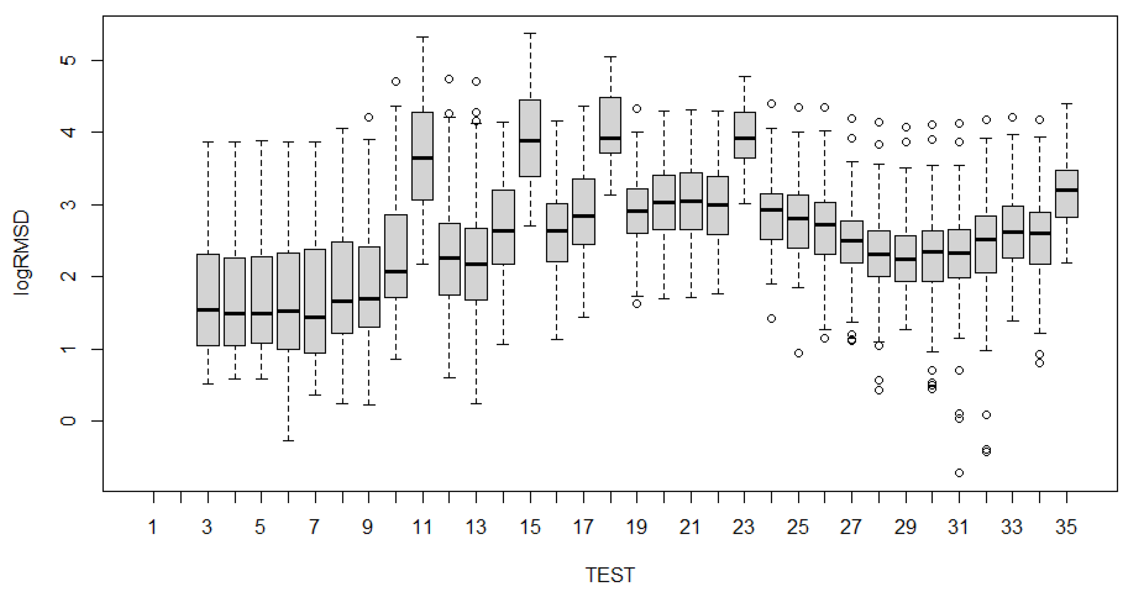
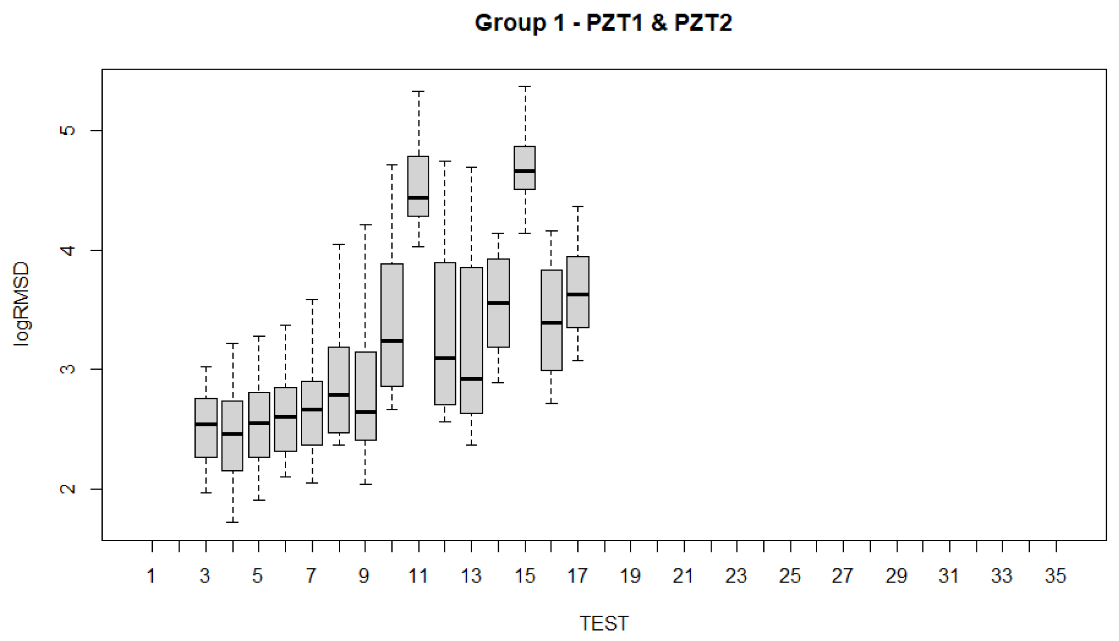
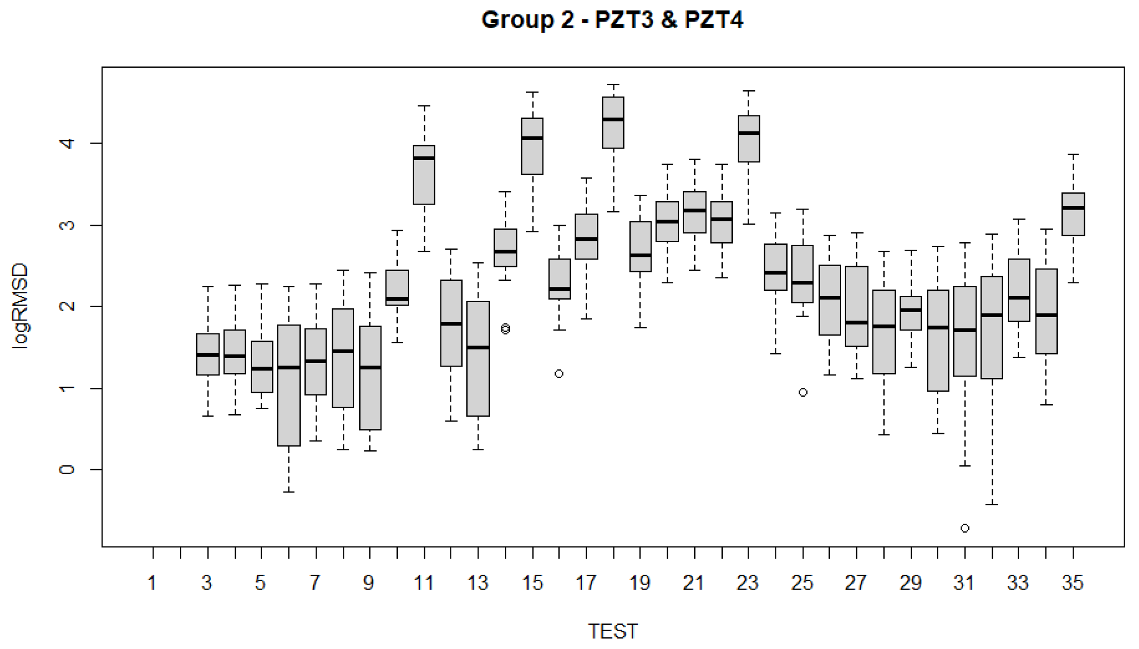
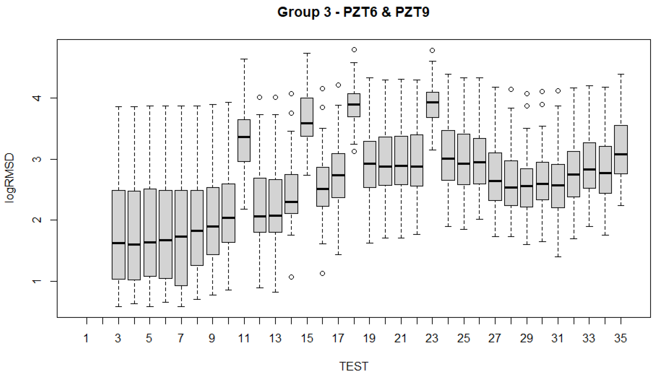
- In general, the observed pattern for all groups of sensors according to the pairwise analysis across the tests is very similar in agreement with the boxplots, except for some differences which will be commented next;
- (b)
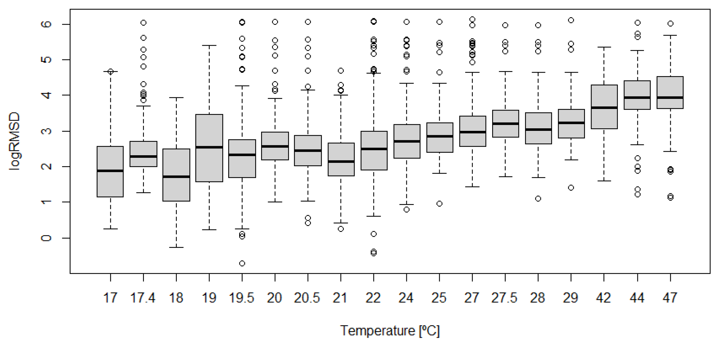
- It is clear that the highest contrast in the p-values appears when heating of the specimen is performed. That high contrast is also shown when the specimen returns to the environmental temperature once its heating is interrupted. Therefore, high temperature variations are perfectly identified with p-values.
- (c)
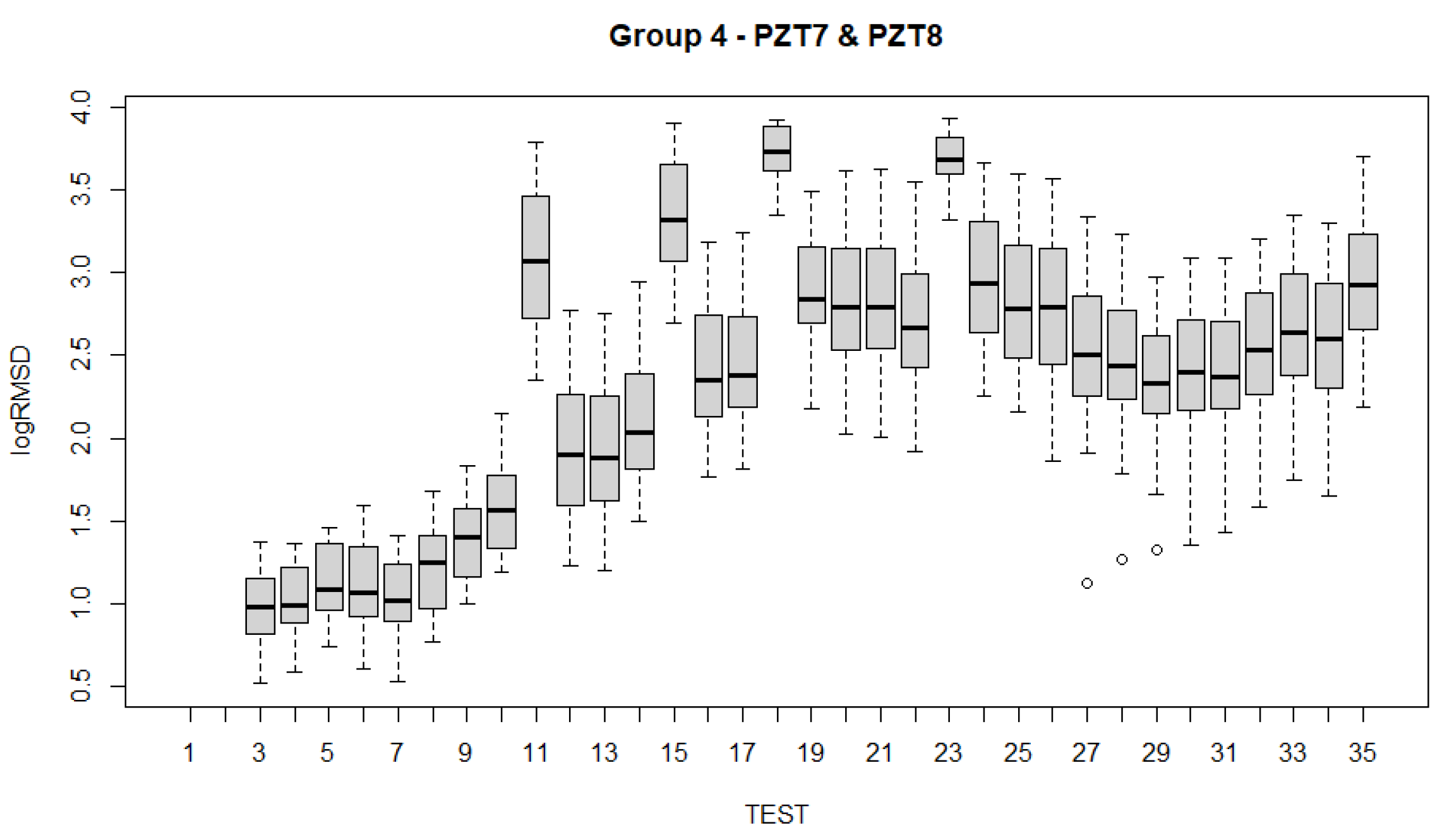
- For the first tests which were performed under a sustained load of 8 kN (tests 3 to 10), there is not a significant difference between consecutive tests except for test 10 when sensors of groups 1, 2 and 4 are considered. This test was the longest test of all those tests carried out under 8 kN and this same conclusion was derived from the boxplots.
- (d)
- When a new sustained load test of 8 kN is performed after the heating and subsequent cooling of the beam, the groups of sensors fail to detect a significant difference in RMSD coefficient, except for group 2 between 13 and 14.
- (e)
- For the sustained load tests under 9.3 kN, no significant difference was detected. The same occurs for the sustained tests under 13.7 kN. In this case, only a clear variation is identified for those sensors bonded to FRP close to the midspan when the beam is initially loaded up to 13.7 kN.
- (f)
- The last load increment until reaching 19.6 kN shows a clear deterioration of the specimen clearly identified by the internal sensors. The much lower p-value in comparison with other previous values, except those due to heating/cooling may be a symptom of severe damage in the structure as the experimental tests demonstrated.
5. Discussion and Conclusions
Author Contributions
Funding
Institutional Review Board Statement
Informed Consent Statement
Data Availability Statement
Conflicts of Interest
References
- Dalfré, G.M.; Barros, J.A.O. NSM technique to increase the load carrying capacity of continuous RC slabs. Eng. Struct. 2013, 56, 137–153. [Google Scholar] [CrossRef] [Green Version]
- Al-Saadi, N.T.K.; Mohammed, A.; Al-Mahaidi, R.; Sanjayan, J. A state-of-the-art review: Near-surface mounted FRP composites for reinforced concrete structures. Constr. Build. Mater. 2019, 209, 748–769. [Google Scholar] [CrossRef]
- Abdallah, M.; Al Mahmoud, F.; Khelil, A.; Mercier, J.; Almassri, B. Assessment of the flexural behavior of continuous RC beams strengthened with NSM-FRP bars, experimental and analytical study. Compos. Struct. 2020, 242, 112127. [Google Scholar] [CrossRef]
- Barris, C.; Sala, P.; Gómez, J.; Torres, L. Flexural behaviour of FRP reinforced concrete beams strengthened with NSM CFRP strips. Compos. Struct. 2020, 241, 112059. [Google Scholar] [CrossRef]
- Suliman, A.K.S.; Jia, Y.; Mohammed, A.A.A. Experimental evaluation of factors affecting the behaviour of reinforced concrete beams strengthened by NSM CFRP strips. Structures 2021, 32, 632–640. [Google Scholar] [CrossRef]
- Emara, M.; Barris, C.; Baena, M.; Torres, L.; Barros, J. Bond behavior of NSM CFRP laminates in concrete under sustained loading. Constr. Build. Mater. 2018, 177, 237–246. [Google Scholar] [CrossRef] [Green Version]
- Gómez, J.; Barris, C.; Jahani, Y.; Baena, M.; Torres, L. Experimental study and numerical prediction of the bond response of NSM CFRP laminates in RC elements under sustained loading. Constr. Build. Mater. 2021, 288, 123082. [Google Scholar] [CrossRef]
- Emara, M.; Torres, L.; Baena, M.; Barris, C.; Cahís, X. Bond response of NSM CFRP strips in concrete under sustained loading and different temperature and humidity conditions. Compos. Struct. 2018, 192, 1–7. [Google Scholar] [CrossRef]
- Del Prete, I.; Bilotta, A.; Bisby, L.; Nigro, E. Elevated temperature response of RC beams strengthened with NSM FRP bars bonded with cementitious grout. Compos. Struct. 2021, 258, 113182. [Google Scholar] [CrossRef]
- Sevillano, E.; Sun, R.; Gil, A.; Perera, R. Interfacial crack-induced debonding identification in FRP-strengthened RC beams from PZT signatures using hierarchical clustering analysis. Compos. Part B Eng. 2016, 87, 322–335. [Google Scholar] [CrossRef]
- Perera, R.; Pérez, A.; García-Diéguez, M.; Zapico-Valle, J.L. Active Wireless System for Structural Health Monitoring Applications. Sensors 2017, 17, 2880. [Google Scholar] [CrossRef] [PubMed] [Green Version]
- Sun, R.; Sevillano, E.; Perera, R. Identification of intermediate debonding damage in FRP-strengthened RC beams based on a multi-objective updating approach and PZT sensors. Compos. Part B Eng. 2017, 109, 248–258. [Google Scholar] [CrossRef]
- Chalioris, C.E.; Kytinou, V.K.; Voutetaki, M.E.; Karayannis, C.G. Flexural Damage Diagnosis in Reinforced Concrete Beams Using a Wireless Admittance Monitoring System-Tests and Finite Element Analysis. Sensors 2021, 21, 679. [Google Scholar] [CrossRef] [PubMed]
- Li, D.; Zhou, J.; Ou, J. Damage, nondestructive evaluation and rehabilitation of FRP composite-RC structure: A review. Constr. Build. Mater. 2021, 271, 121551. [Google Scholar] [CrossRef]
- Perera, R.; Torres, L.; Ruiz, A.; Barris, C.; Baena, M. An EMI-Based Clustering for Structural Health Monitoring of NSM FRP Strengthening Systems. Sensors 2019, 19, 3775. [Google Scholar] [CrossRef] [Green Version]
- Hameed, M.S.; Li, Z.; Chen, J.; Qi, J. Lamb-Wave-Based Multistage Damage Detection Method Using an Active PZT Sensor Network for Large Structures. Sensors 2019, 19, 2010. [Google Scholar] [CrossRef] [Green Version]
- Na, W.S.; Baek, J. A review of the piezoelectric electromechanical impedance based structural health monitoring technique for engineering structures. Sensors 2018, 18, 1307. [Google Scholar] [CrossRef] [Green Version]
- Welch, K.B.; Galecki, A.T.; West, B.T. Linear Mixed Models. A Practical Guide Using Statistical Software, 2nd ed.; Champan and Hall/CRC: New York, NY, USA, 2014. [Google Scholar]
- Faraway, J.J. Extending the Linear Model with R: Generalized Linear, Mixed Effects, and Nonparametric Regression Models, 2nd ed.; Champan and Hall/CRC: New York, NY, USA, 2016. [Google Scholar]
- Harrison, X.A.; Donaldson, L.; Correa-Cano, M.E.; Evans, J.; Fisher, D.N.; Goodwin, C.E.D.; Robinson, B.S.; Hodgson, D.J.; Inger, R. A brief introduction to mixed effects modelling and multi-model inference in ecology. PeerJ 2018, 6, 4794. [Google Scholar] [CrossRef] [PubMed] [Green Version]
- Meteyard, L.; Davies, R.A.I. Best practice guidance for linear mixed-effects models in psychological science. J. Mem. Lang. 2020, 112, 104092. [Google Scholar] [CrossRef] [Green Version]
- Graves, C.E.; Hwang, R.; McManus, C.M.; Lee, J.A.; Kuo, J.H. The effect of chronic kidney disease on intraoperative parathyroid hormone: A linear mixed model analysis. Surgery 2021, 169, 1152–1157. [Google Scholar] [CrossRef]
- Perera, R.; Gil, A.; Torres, L.; Barris, C. Diagnosis of NSM FRP reinforcement in concrete by using mixed-effects models and EMI approaches. Compos. Struct. 2021, 273, 114322. [Google Scholar] [CrossRef]
- Liang, C.; Sun, F.; Rogers, C.A. Electro-mechanical impedance modeling of active material systems. Smart Mater. Struct. 1994, 21, 232–252. [Google Scholar] [CrossRef]
- PI Piezo Technology. DuraAct Patch Transducer. Available online: https://www.piceramic.com/en/products/piezoceramic-actuators/patch-transducers/ (accessed on 8 June 2021).
- RStudio Desktop. Available online: http://www.rstudio.com/ (accessed on 11 June 2021).
- Pinheiro, J.C.; Bates, D.M. Mixed Effects Models in S and S-Plus (Statistics and Computing); Springer: New York, NY, USA, 2000. [Google Scholar]


| Test Number | dd/mm/yyyy | Sustained Load Level [kN] | Loading Test Duration [days] | Test Temperature [°C] | |
|---|---|---|---|---|---|
| 0 | 08/01/2018 | 0 | - | NA | NA |
| 1 | 11/01/2018 | 8 | 2 | 17 | Environmental |
| 2 | 25/01/2018 | 8 | 7 | 19 | Environmental |
| 3 | 08/02/2018 | 8 | 14 | 17 | Environmental |
| 4 | 13/02/2018 | 8 | 4 | 17 | Environmental |
| 5 | 15/02/2018 | 8 | 1.5 | 17 | Environmental |
| 6 | 19/02/2018 | 8 | 3 | 18 | Environmental |
| 7 | 22/02/2018 | 0 | 3 | 18 | Environmental |
| 8 | 12/03/2018 | 8 | 14 | 19.5 | Environmental |
| 9 | 03/04/2018 | 8 | 21 | 19 | Environmental |
| 10 | 24/04/2018 | 8 | 21 | 22 | Environmental |
| 11 | 26/04/2018 | 0 | 1 | 42 | Heated |
| 12 | 30/04/2018 | 0 | 3 | 22 | Environmental |
| 13 | 03/05/2018 | 0 | 3 | 21 | Environmental |
| 14 | 27/05/2018 | 8 | 23 | 24 | Environmental |
| 15 | 31/05/2018 | 0 | 3 | 42 | Heated |
| 16 | 01/06/2018 | 0 | 2 | 24 | Environmental |
| 17 | 02/07/2018 | 8 | 30 | 27 | Environmental |
| 18 | 05/07/2018 | 0 | 3 | 47 | Heated |
| 19 | 09/07/2018 | 0 | 3 | 27 | Environmental |
| 20 | 25/07/2018 | 8 | 14 | 28 | Environmental |
| 21 | 26/07/2018 | 9.3 | 1 | 27.5 | Environmental |
| 22 | 04/09/2018 | 9.3 | 31 | 27 | Environmental |
| 23 | 05/09/2018 | 0 | 1 | 44 | Heated |
| 24 | 07/09/2018 | 0 | 3 | 27 | Environmental |
| 25 | 06/10/2018 | 9.3 | 21 | 25 | Environmental |
| 26 | 07/10/2018 | 13.7 | 1 | 22 | Environmental |
| 27 | 06/11/2018 | 13.7 | 28 | 20 | Environmental |
| 28 | 04/12/2018 | 13.7 | 29 | 20.5 | Environmental |
| 29 | 04/02/2019 | 13.7 | 60 | 17.4 | Environmental |
| 30 | 13/03/2019 | 13.7 | 41 | 19.5 | Environmental |
| 31 | 14/03/2019 | 17.7 | 1 | 19.5 | Environmental |
| 32 | 13/05/2019 | 17.7 | 60 | 22 | Environmental |
| 33 | 10/06/2019 | 17.7 | 30 | 24 | Environmental |
| 34 | 13/06/2019 | 19.6 | 2 | 24 | Environmental |
| 35 | 27/07/2019 | 19.6 | 42 | 29 | Environmental |
| Test number | 3 | 4 | 5 | 6 | 7 | 8 | 9 |
| p-value | 0.0676121 | 0.17934489 | 0.07940822 | 0.46347637 | 0.10371856 | 0.15253014 | 0.28992103 |
| Test number | 10 | 11 | 12 | 13 | 14 | 15 | 16 |
| p-value | 0.0568042 | 0.81895703 | 0.60769883 | 0.49746651 | 0.91459634 | 0.79595994 | 0.69038784 |
| Test number | 17 | 18 | 19 | 20 | 21 | 22 | 23 |
| p-value | 0.86443078 | 0.36518012 | 0.9042454 | 0.89197109 | 0.96226618 | 0.90848409 | 0.91443105 |
| Test number | 24 | 25 | 26 | 27 | 28 | 29 | 30 |
| p-value | 0.85373292 | 0.95754631 | 0.70759643 | 0.5601079 | 0.43779154 | 0.73708194 | 0.49989917 |
| Test number | 31 | 32 | 33 | 34 | 35 | ||
| p-value | 0.05344414 | 0.04345163 | 0.84320087 | 0.33456275 | 0.95263826 |
| Group Number | p-Value |
|---|---|
| All sensors | 0.05832 |
| 1 | 0.04118 |
| 2 | 0.06561 |
| 3 | 0.7728 |
| 4 | 0.0085 |
| All Sensors | Group 1 | Group 2 | Group 3 | Group 4 | |
|---|---|---|---|---|---|
| Variations | <2.2 × 10⁻¹⁶ | 2.0 × 10⁻¹⁶ | 2.0 × 10⁻¹⁶ | 2.0 × 10⁻¹⁶ | 2.0 × 10⁻¹⁶ |
| Frequency | 1 | 0.99999 | 0.99879 | 1 | 2.0 × 10⁻¹⁶ |
| Tests | p-Value | ||||
|---|---|---|---|---|---|
| All Sensors | Group 1 | Group 2 | Group 3 | Group 4 | |
| 3–4 | 1 | 1 | 1 | 1 | 1 |
| 4–5 | 1 | 1 | 1 | 1 | 1 |
| 5–6 | 1 | 1 | 1 | 1 | 1 |
| 6–7 | 1 | 1 | 1 | 1 | 1 |
| 7–8 | 1 | 1 | 1 | 1 | 0.013256 |
| 8–9 | 1 | 1 | 1 | 1 | 0.459903 |
| 9–10 | 0.00000189 | 0.000224 | 0.000013 | 1 | 0.036852 |
| 10–11 | <2 × 10⁻¹⁶ | 8.67 × 10⁻¹² | 7.11 × 10⁻¹³ | 0.00000351 | 2 × 10⁻¹⁶ |
| 11–12 | <2 × 10⁻¹⁶ | 2.26 × 10⁻¹³ | 2 × 10⁻¹⁶ | 0.0000437 | 2 × 10⁻¹⁶ |
| 12–13 | 1 | 1 | 1 | 1 | 1 |
| 13–14 | 0.00000716 | 0.778527 | 1.52 × 10⁻⁸ | 1 | 0.09984 |
| 14–15 | <2 × 10⁻¹⁶ | 4.42 × 10⁻¹³ | 7.57 × 10⁻¹⁰ | 0.00000138 | 2 × 10⁻¹⁶ |
| 15–16 | <2 × 10⁻¹⁶ | 2 × 10⁻¹⁶ | 2 × 10⁻¹⁶ | 0.0000519 | 2 × 10⁻¹⁶ |
| 16–17 | 0.280975 | 0.977147 | 0.449131 | 1 | 1 |
| 17–18 | <2 × 10⁻¹⁶ | 3.35 × 10⁻¹¹ | 0.00000479 | 2 × 10⁻¹⁶ | |
| 18–19 | <2 × 10⁻¹⁶ | 9.06 × 10⁻¹⁴ | 0.000369 | 2 × 10⁻¹⁶ | |
| 19–20 | 1 | 1 | 1 | 1 | |
| 20–21 | 1 | 1 | 1 | 1 | |
| 21–22 | 1 | 1 | 1 | 1 | |
| 22–23 | <2 × 10⁻¹⁶ | 0.0000125 | 0.000254 | 2 × 10⁻¹⁶ | |
| 23–24 | <2 × 10⁻¹⁶ | 2 × 10⁻¹⁶ | 0.003112 | 2 × 10⁻¹⁶ | |
| 24–25 | 1 | 1 | 1 | 0.541478 | |
| 25–26 | 1 | 1 | 1 | 1 | |
| 26–27 | 1 | 1 | 1 | 0.0000966 | |
| 27–28 | 1 | 1 | 1 | 1 | |
| 28–29 | 1 | 1 | 1 | 1 | |
| 29–30 | 1 | 1 | 1 | 1 | |
| 30–31 | 1 | 1 | 1 | 1 | |
| 31–32 | 1 | 1 | 1 | 0.569178 | |
| 32–33 | 0.494927 | 0.263567 | 1 | 1 | |
| 33–34 | 1 | 1 | 1 | 1 | |
| 34–35 | 6.22 × 10⁻¹¹ | 4.85 × 10⁻⁹ | 1 | 3.8 × 10⁻⁸ | |
Publisher’s Note: MDPI stays neutral with regard to jurisdictional claims in published maps and institutional affiliations. |
© 2021 by the authors. Licensee MDPI, Basel, Switzerland. This article is an open access article distributed under the terms and conditions of the Creative Commons Attribution (CC BY) license (https://creativecommons.org/licenses/by/4.0/).
Share and Cite
Perera, R.; Torres, L.; Díaz, F.J.; Barris, C.; Baena, M. Performance of Linear Mixed Models to Assess the Effect of Sustained Loading and Variable Temperature on Concrete Beams Strengthened with NSM-FRP. Sensors 2021, 21, 5046. https://doi.org/10.3390/s21155046
Perera R, Torres L, Díaz FJ, Barris C, Baena M. Performance of Linear Mixed Models to Assess the Effect of Sustained Loading and Variable Temperature on Concrete Beams Strengthened with NSM-FRP. Sensors. 2021; 21(15):5046. https://doi.org/10.3390/s21155046
Chicago/Turabian StylePerera, Ricardo, Lluis Torres, Francisco J. Díaz, Cristina Barris, and Marta Baena. 2021. "Performance of Linear Mixed Models to Assess the Effect of Sustained Loading and Variable Temperature on Concrete Beams Strengthened with NSM-FRP" Sensors 21, no. 15: 5046. https://doi.org/10.3390/s21155046