
Increasing the Reliability of Data Collection of Laser Line Triangulation Sensor by Proper Placement of the Sensor

 , , , , and
Abstract
:1. Introduction
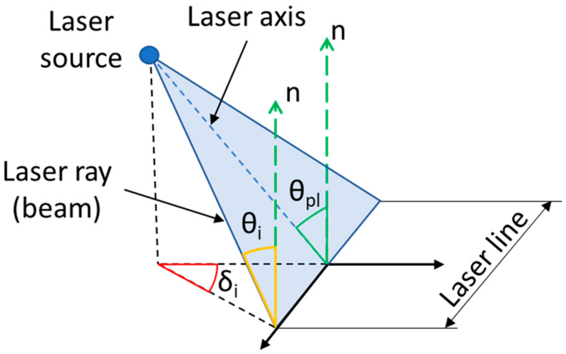
2. Methodology
3. Experiment Setup and Details
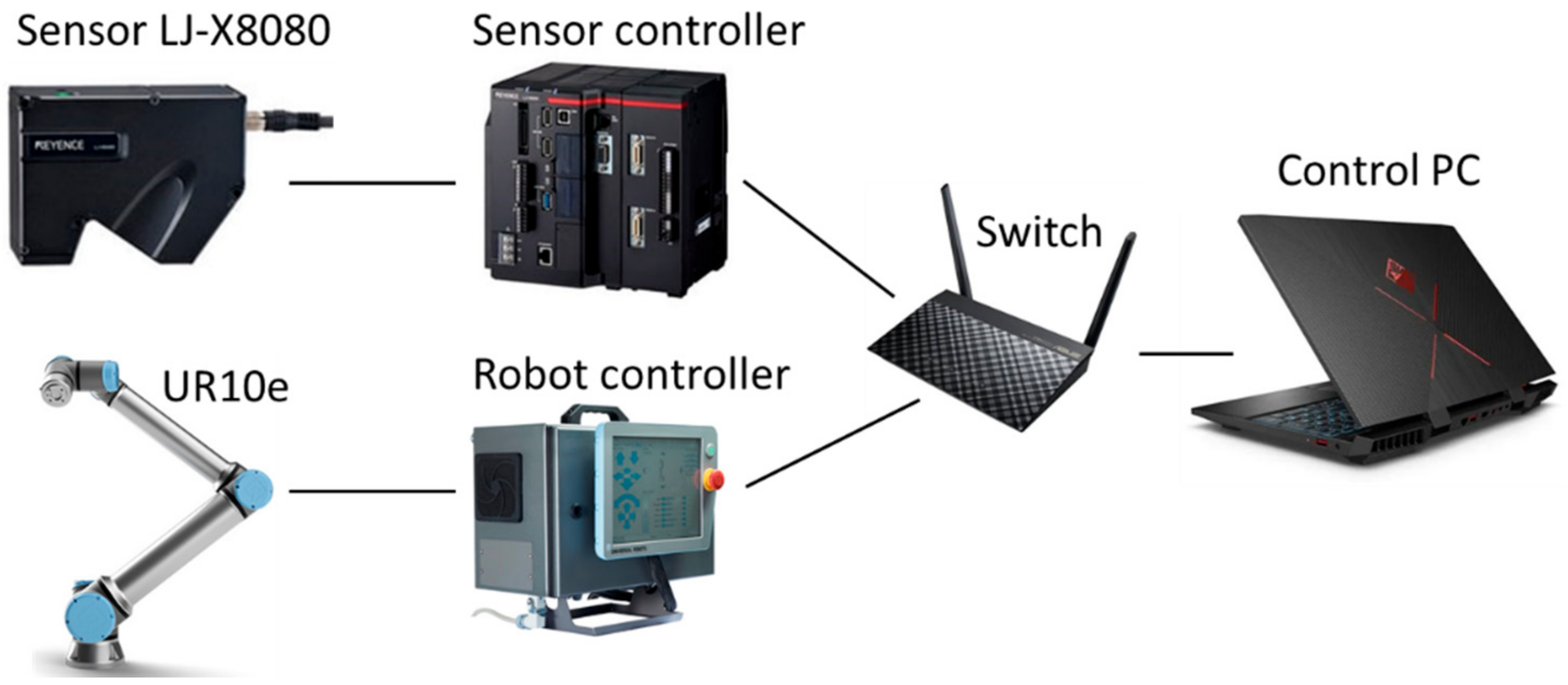
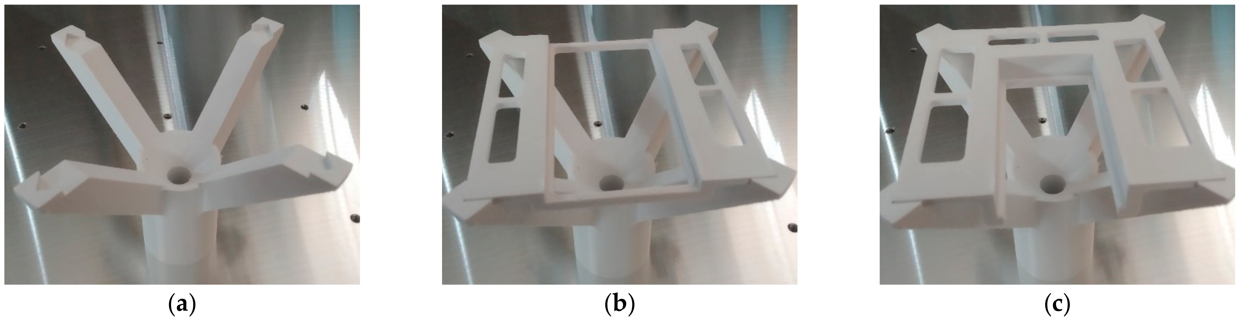
3.1. Experimental Workplace
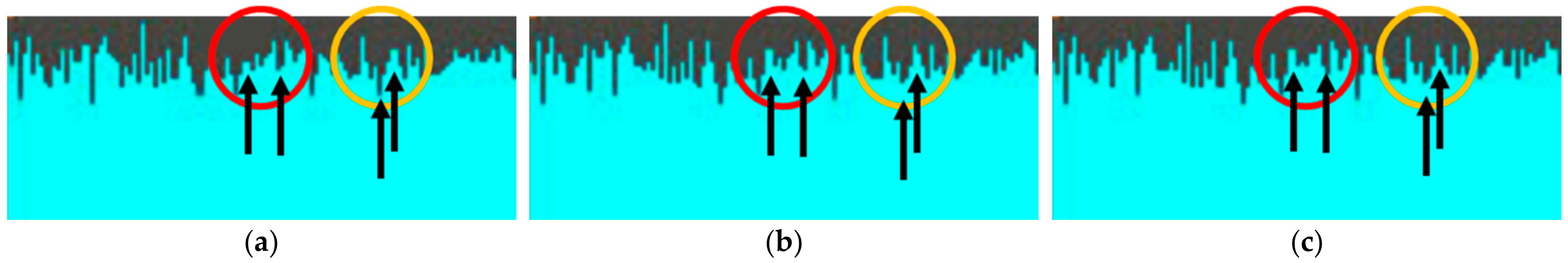
3.2. Data Collection
| Algorithm 1. The measurement process. |
| for i = 0 to m // m[1:140] represents the position (pose) number, each position corresponds to a specific AoI set_robot_pose (i) waittime // stabilization of the robot for j = 0 to n // n[1:30] represents the number of frames in one position Get profile data Get image data Save data end for Get mean profile data Get mean intensity data end for |
| Algorithm 2. Acquisition of reflected intensity data. |
| for i = 0 to m // m[1:140] represents a saved scan that corresponds to a certain pose of the sensor for j = 0 to n // n[1:3200] represents the point ID number in the saved profile if n exists get_angle_of_incidence (j) assign_intensity_to_point (j) end if end for Save data end for |
4. Results
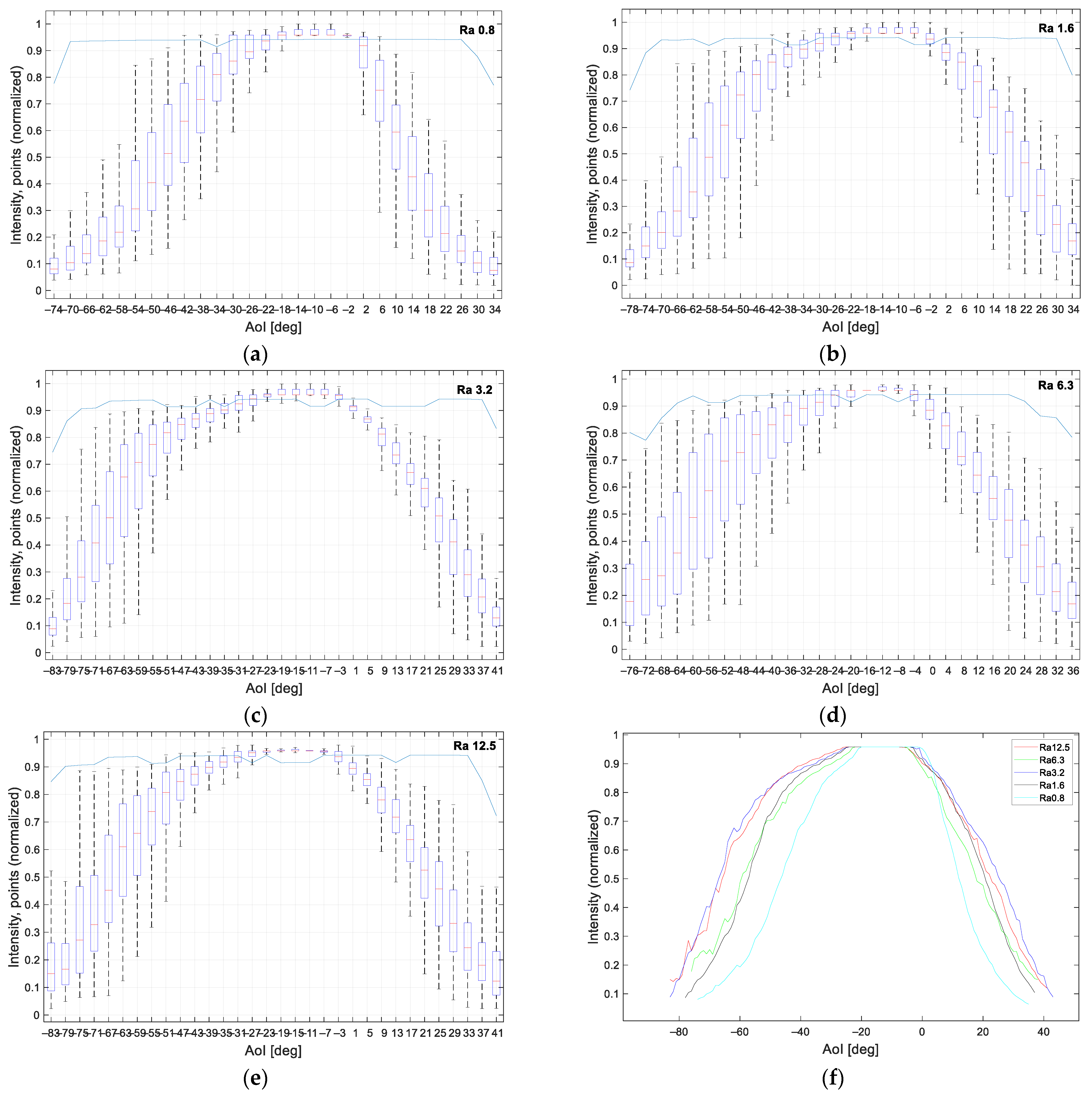
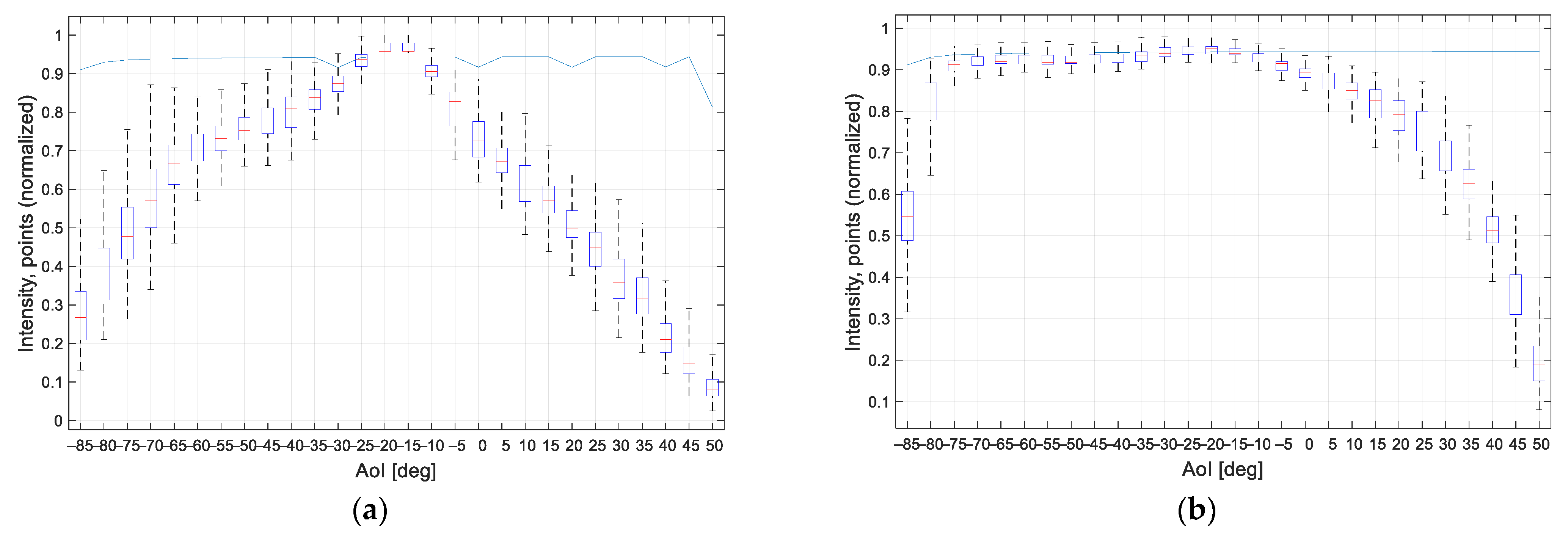
4.1. Aluminum Alloy with Different Roughness
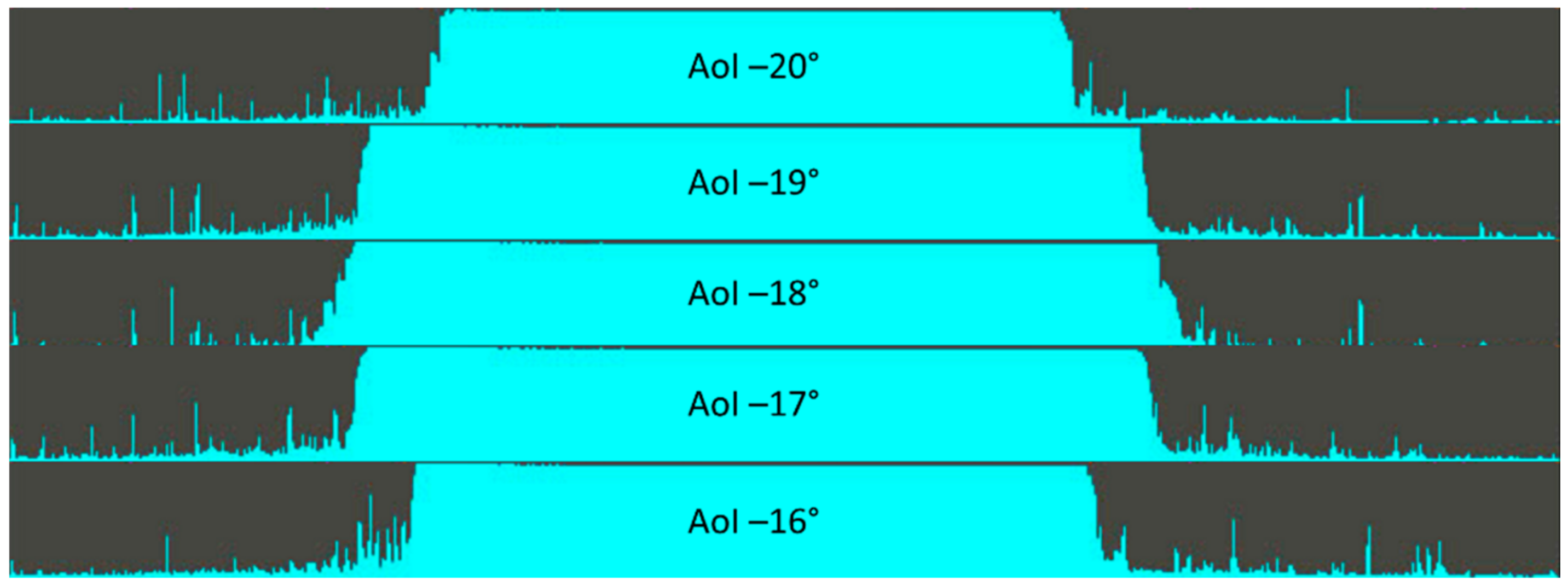
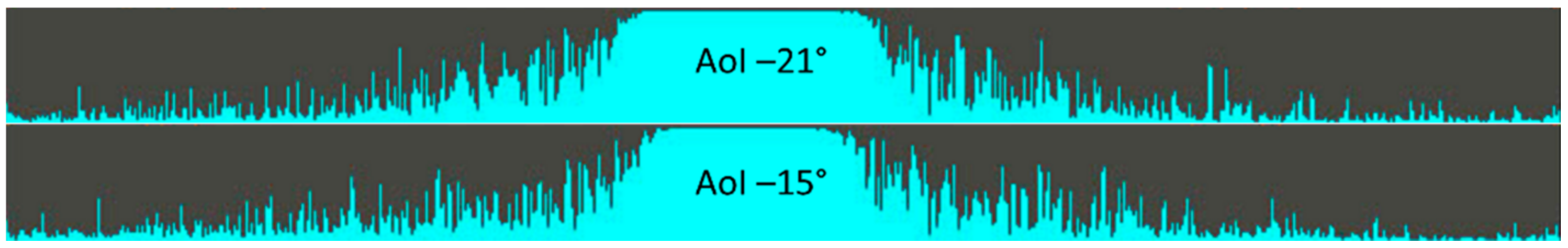
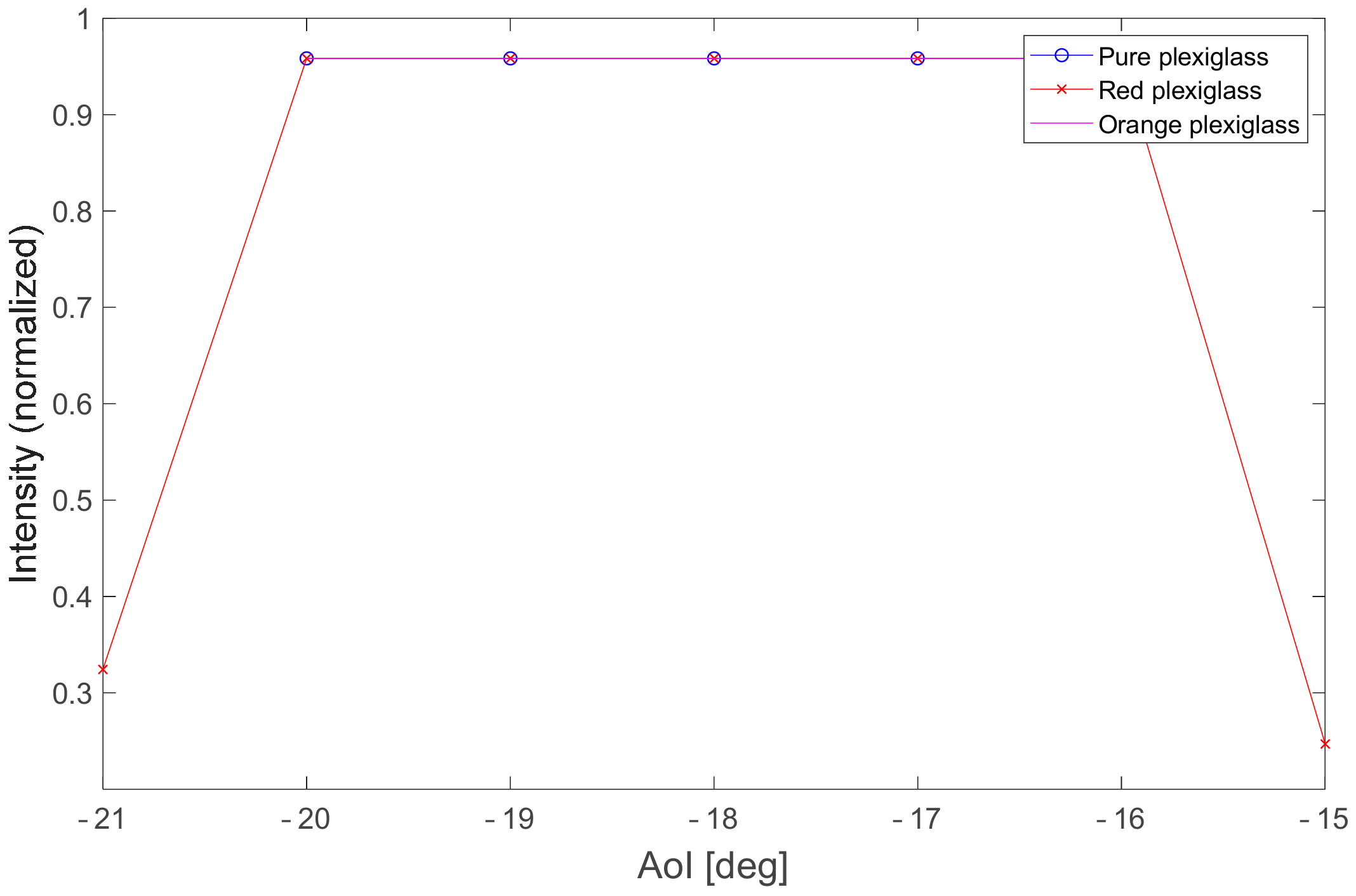
4.2. Transparent Plastics
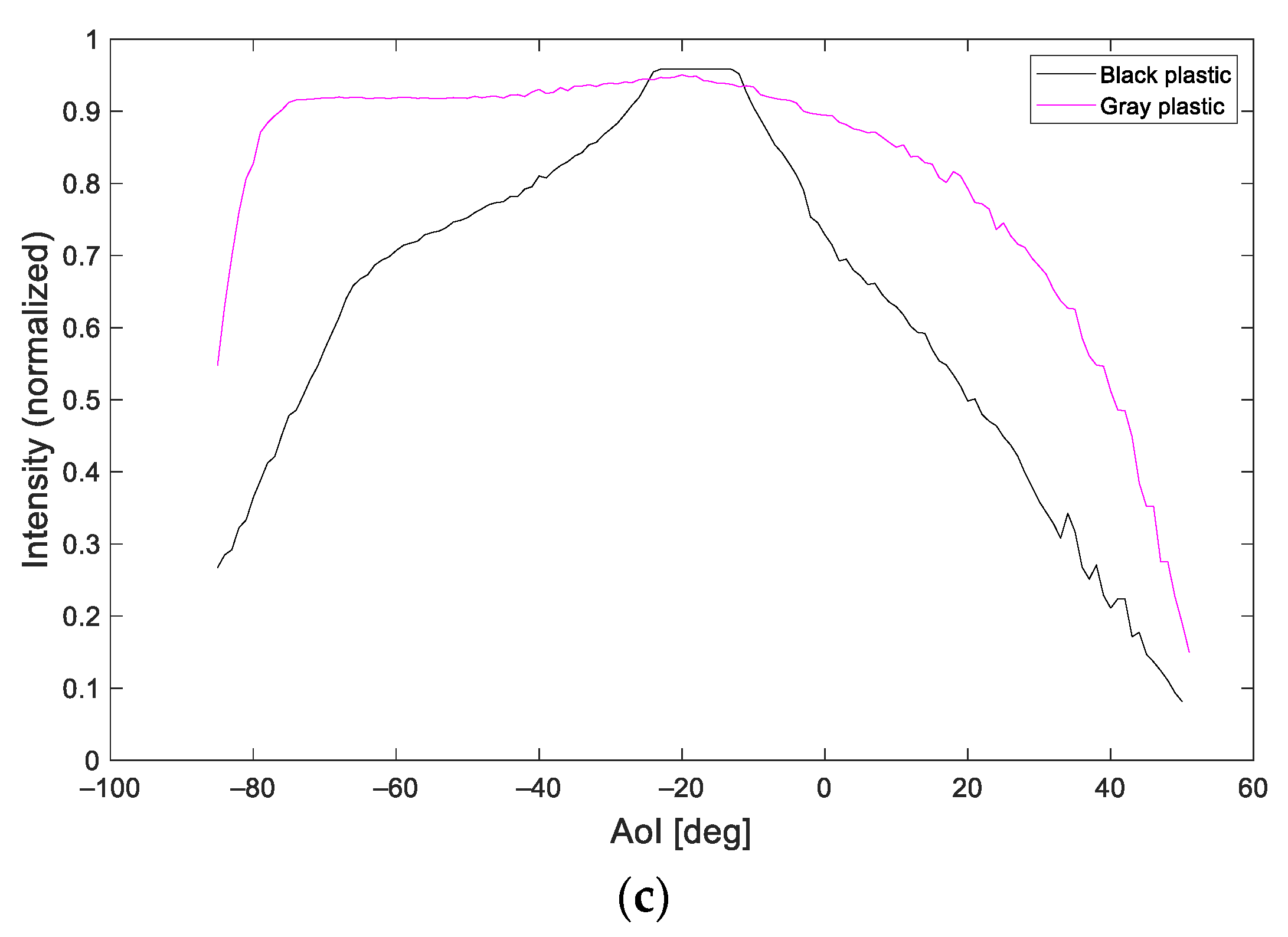
4.3. Non-Transparent Plastics and Overview
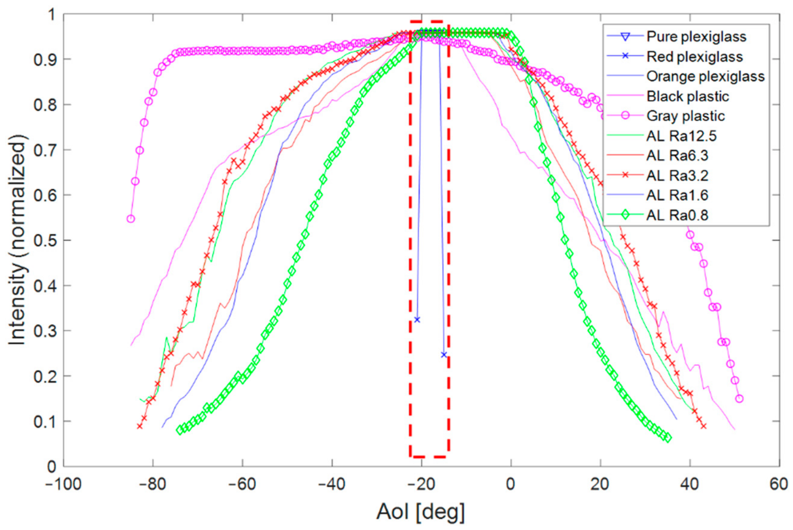
4.4. The Results Overview
5. Conclusions
Author Contributions
Funding
Institutional Review Board Statement
Informed Consent Statement
Data Availability Statement
Conflicts of Interest
Abbreviations
| AoI | Angle of incidence |
| LLT | Laser line triangulation |
| CCD | Charge-coupled device |
| DoF | Degrees of freedom |
References
- Balduzzi, M.A.; Van Der Zande, D.; Stuckens, J.; Verstraeten, W.W.; Coppin, P. The Properties of Terrestrial Laser System Intensity for Measuring Leaf Geometries: A Case Study with Conference Pear Trees (Pyrus Communis). Sensors 2011, 11, 1657–1681. [Google Scholar] [CrossRef]
- Albano, R. Investigation on Roof Segmentation for 3D Building Reconstruction from Aerial LIDAR Point Clouds. Appl. Sci. 2019, 9, 4674. [Google Scholar] [CrossRef] [Green Version]
- Kus, A. Implementation of 3D Optical Scanning Technology for Automotive Applications. Sensors 2009, 9, 1967–1979. [Google Scholar] [CrossRef] [PubMed]
- Li, F.; Longstaff, A.P.; Fletcher, S.; Myers, A. Rapid and accurate reverse engineering of geometry based on a multi-sensor system. Int. J. Adv. Manuf. Technol. 2014, 74, 369–382. [Google Scholar] [CrossRef] [Green Version]
- Chang, W.-C.; Wu, C.-H. Eye-in-hand vision-based robotic bin-picking with active laser projection. Int. J. Adv. Manuf. Technol. 2016, 85, 2873–2885. [Google Scholar] [CrossRef]
- Wu, X.; Li, Z.; Wen, P. An automatic shoe-groove feature extraction method based on robot and structural laser scanning. Int. J. Adv. Robot. Syst. 2017, 14. [Google Scholar] [CrossRef]
- Zhang, M.; Shi, H.; Yu, Y.; Zhou, M. A Computer Vision Based Conveyor Deviation Detection System. Appl. Sci. 2020, 10, 2402. [Google Scholar] [CrossRef] [Green Version]
- Na, K.-M.; Lee, K.; Shin, S.-K.; Kim, H. Detecting Deformation on Pantograph Contact Strip of Railway Vehicle on Image Processing and Deep Learning. Appl. Sci. 2020, 10, 8509. [Google Scholar] [CrossRef]
- Wang, Z.; Zhang, C.; Pan, Z.; Wang, Z.; Liu, L.; Qi, X.; Mao, S.; Pan, J. Image Segmentation Approaches for Weld Pool Monitoring during Robotic Arc Welding. Appl. Sci. 2018, 8, 2445. [Google Scholar] [CrossRef] [Green Version]
- Bickel, G.; Häusler, G.; Maul, M. Triangulation with Expanded Range of Depth. Opt. Eng. 1985, 24, 246975. [Google Scholar] [CrossRef]
- Dong, Z.; Sun, X.; Liu, W.; Yang, H. Measurement of Free-Form Curved Surfaces Using Laser Triangulation. Sensors 2018, 18, 3527. [Google Scholar] [CrossRef] [Green Version]
- Wang, Y.; Feng, H.-Y. Effects of scanning orientation on outlier formation in 3D laser scanning of reflective surfaces. Opt. Lasers Eng. 2016, 81, 35–45. [Google Scholar] [CrossRef]
- Van Gestel, N.; Cuypers, S.; Bleys, P.; Kruth, J.-P. A performance evaluation test for laser line scanners on CMMs. Opt. Lasers Eng. 2009, 47, 336–342. [Google Scholar] [CrossRef] [Green Version]
- Gao, F.; Muhamedsalih, H.; Jiang, X. Surface and thickness measurement of a transparent film using wavelength scanning interferometry. Opt. Express 2012, 20, 21450–21456. [Google Scholar] [CrossRef] [PubMed] [Green Version]
- Ran, R.; Stolz, C.; Fofi, D.; Meriaudeau, F. Non contact 3D measurement scheme for transparent objects using UV structured light 2010. In Proceedings of the 2010 20th International Conference on Pattern Recognition, Istanbul, Turkey, 23–26 August 2010; pp. 1646–1649. [Google Scholar] [CrossRef]
- Bonfort, T.; Sturm, P.; Gargallo, P. General Specular Surface Triangulation. In Lecture Notes in Computer Science (Including Subseries Lecture Notes in Artificial Intelligence and Lecture Notes in Bioinformatics); Springer: Hyderabad, India, 2006; Volume 3852, pp. 872–881. [Google Scholar] [CrossRef]
- Weinmann, M.; Osep, A.; Ruiters, R.; Klein, R. Multi-View Normal Field Integration for 3D Reconstruction of Mirroring Objects. In Proceedings of the 2013 IEEE International Conference on Computer Vision, Sydney, NSW, Australia, 1–8 December 2013; pp. 2504–2511. [Google Scholar] [CrossRef]
- Ihrke, I.; Kutulakos, K.N.; Lensch, H.P.A.; Magnor, M.; Heidrich, W. Transparent and Specular Object Reconstruction. Comput. Graph. Forum 2010, 29, 2400–2426. [Google Scholar] [CrossRef]
- Mian, S.H.; Mannan, M.A.; Al-Ahmari, A.M. The influence of surface topology on the quality of the point cloud data acquired with laser line scanning probe. Sens. Rev. 2014, 34, 255–265. [Google Scholar] [CrossRef]
- Weyrich, T.; Pauly, M.; Keiser, R.; Heinzle, S.; Gross, M. Post-processing of Scanned 3D Surface Data. Eurographics Symp. Point-Based Graph. 2004, 1. [Google Scholar] [CrossRef]
- Tan, K.; Cheng, X. Specular Reflection Effects Elimination in Terrestrial Laser Scanning Intensity Data Using Phong Model. Remote. Sens. 2017, 9, 853. [Google Scholar] [CrossRef] [Green Version]
- Oren, M.; Nayar, S.K. Generalization of the Lambertian model and implications for machine vision. Int. J. Comput. Vis. 1995, 14, 227–251. [Google Scholar] [CrossRef]
- Nayar, S.; Ikeuchi, K.; Kanade, T. Surface reflection: Physical and geometrical perspectives. IEEE Trans. Pattern Anal. Mach. Intell. 1991, 13, 611–634. [Google Scholar] [CrossRef] [Green Version]
- Vukašinović, N.; Korošec, M.; Duhovnik, J. The influence of surface topology on the accuracy of laser triangulation scanning results. Stroj. Vestn. J. Mech. Eng. 2010, 56, 23–30. [Google Scholar]
- Li, L.H.; Yu, N.H.; Chan, C.Y.; Lee, W.B. Al6061 surface roughness and optical reflectance when machined by single point diamond turning at a low feed rate. PLoS ONE 2018, 13, e0195083. [Google Scholar] [CrossRef] [PubMed] [Green Version]
- Cuesta, E.; Rico, J.C.; Fernández, J.C.R.; Blanco, D.; Valiño, G. Influence of roughness on surface scanning by means of a laser stripe system. Int. J. Adv. Manuf. Technol. 2009, 43, 1157–1166. [Google Scholar] [CrossRef]
- Blanco, D.; Fernandez, P.J.P.; Valiño, G.; Rico, J.C.; Rodriguez, A.L.P.; Segui, V.J. Influence of ambient light on the repeatability of laser triangulation digitized point clouds when scanning EN AW 6082 flat faced features. Third Manuf. Eng. Soc. Int. Conf. MESIC-09 2009, 1181, 509–520. [Google Scholar] [CrossRef]
- Blanco, D.; Fernández, D.B.; Cuesta, E.; Mateos, S.; Beltran, N. Influence of surface material on the quality of laser triangulation digitized point clouds for reverse engineering tasks. In 2009 IEEE Conference on Emerging Technologies Factory Automation; IEEE: New York, NY, USA; pp. 1–8. [CrossRef]
- Serway, R.A.; Jewett, J.W. Energy Transfer Mechanisms in Thermal Processes. In Physics for Scientists and Engineers with Modern Physics, 10th ed.; Cengage Learning: Boston, MA, USA, 2018; pp. 522–525. [Google Scholar]


| Parameter | Specification |
|---|---|
| DoF | 6 |
| Reach | 1300 mm |
| Payload | 10 kg |
| Pose repeatability | ±0.05 mm |
| Parameter | Specification |
|---|---|
| Reference distance (Z-axis) | 73 mm |
| Triangulation angle | 35° |
| Measuring range (Z-axis) | ±20.5 mm (full scale = 41 mm) |
| Measuring range (X-axis) | 30 mm (near side) |
| 35 mm (reference distance) | |
| 39 (far side) | |
| Linearity (Z-axis) | ±0.03% of the full scale |
| Profile data count | 3 200 points |
| Laser type | Blue laser |
| Laser source | 10 mW |
| Laser wavelength | 405 nm (visible light) |
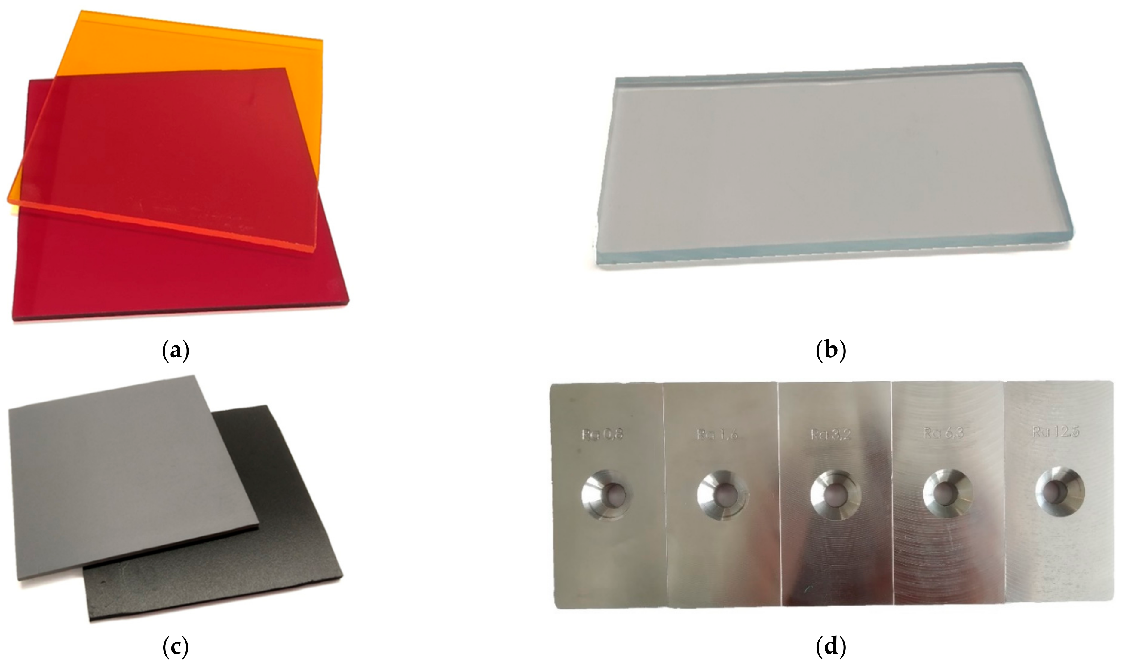
| Material | Width [mm] | Height [mm] | Thickness [mm] | Roughness [µm] | Flatness [mm] |
|---|---|---|---|---|---|
| Non-transparent plastics | 100 | 100 | 3 | Ra1.2 | 0.02 |
| Colored transparent plastics | 100 | 100 | 3 | Ra0.01–0.04 | 0.01 |
| Pure transparent plastic | 50 | 100 | 5 | Ra0.01–0.04 | 0.01 |
| Aluminum alloy | 40 | 80 | 12 | Ra0.8, 1.6, 3.2, 6.3, 12.5 | 0.02 |
| AoI | Median | Mean | 25th Percentile | 75th Percentile |
|---|---|---|---|---|
| −21° | 0.324 | 0.445 | 0.133 | 0.875 |
| −20° | 0.958 | 0.597 | 0.158 | 0.958 |
| −19° | 0.958 | 0.691 | 0.259 | 0.958 |
| −18° | 0.958 | 0.716 | 0.320 | 0.958 |
| −17° | 0.958 | 0.675 | 0.241 | 0.958 |
| −16° | 0.958 | 0.633 | 0.191 | 0.958 |
| −15° | 0.310 | 0.428 | 0.134 | 0.785 |
| AoI | Median | Mean | 25th Percentile | 75th Percentile |
|---|---|---|---|---|
| −20° | 0.958 | 0.815 | 0.958 | 0.958 |
| −19° | 0.958 | 0.880 | 0.958 | 0.958 |
| −18° | 0.958 | 0.854 | 0.958 | 0.958 |
| −17° | 0.958 | 0.865 | 0.958 | 0.958 |
| −16° | 0.958 | 0.822 | 0.958 | 0.958 |
| AoI | Median | Mean | 25th Percentile | 75th Percentile |
|---|---|---|---|---|
| −20° | 0.958 | 0.929 | 0.958 | 0.958 |
| −19° | 0.958 | 0.961 | 0.958 | 0.958 |
| −18° | 0.958 | 0.960 | 0.958 | 0.958 |
| −17° | 0.958 | 0.962 | 0.958 | 0.958 |
| −16° | 0.958 | 0.961 | 0.958 | 0.958 |
| Material | Detection Range | Recommended Range |
|---|---|---|
| Aluminum alloy Ra0.8 | [−74°, 34°] | [−21°, 0°] |
| Aluminum alloy Ra1.6 | [−78°, 34°] | [−25°, −1°] |
| Aluminum alloy Ra3.2 | [−83°, 41°] | [−26°, 0°] |
| Aluminum alloy Ra6.3 | [−76°, 36°] | [−24°, −3°] |
| Aluminum alloy Ra12.5 | [−83°, 41°] | [−30°, −1°] |
| Pure transparent plastic | [−20°, −16°] | [−20°, −16°] |
| Orange transparent plastic | [−20°, −16°] | [−20°, −16°] |
| Red transparent plastic | [−21°, −15°] | [−20°, −16°] |
| Black non-transparent plastic | [−85°, 50°] | [−25°, −11°] |
| Gray non-transparent plastic | [−85°, 50°] | [−80°, 0°] |
Publisher’s Note: MDPI stays neutral with regard to jurisdictional claims in published maps and institutional affiliations. |
© 2021 by the authors. Licensee MDPI, Basel, Switzerland. This article is an open access article distributed under the terms and conditions of the Creative Commons Attribution (CC BY) license (https://creativecommons.org/licenses/by/4.0/).
Share and Cite
Heczko, D.; Oščádal, P.; Kot, T.; Huczala, D.; Semjon, J.; Bobovský, Z. Increasing the Reliability of Data Collection of Laser Line Triangulation Sensor by Proper Placement of the Sensor. Sensors 2021, 21, 2890. https://doi.org/10.3390/s21082890
Heczko D, Oščádal P, Kot T, Huczala D, Semjon J, Bobovský Z. Increasing the Reliability of Data Collection of Laser Line Triangulation Sensor by Proper Placement of the Sensor. Sensors. 2021; 21(8):2890. https://doi.org/10.3390/s21082890
Chicago/Turabian StyleHeczko, Dominik, Petr Oščádal, Tomáš Kot, Daniel Huczala, Ján Semjon, and Zdenko Bobovský. 2021. "Increasing the Reliability of Data Collection of Laser Line Triangulation Sensor by Proper Placement of the Sensor" Sensors 21, no. 8: 2890. https://doi.org/10.3390/s21082890