Deep Learning Applied to Phenotyping of Biomass in Forages with UAV-Based RGB Imagery

 , , ,
, , ,  , ,
, ,  , , , , ,
  ,
,  and
and 
Abstract
:1. Introduction
2. Materials and Methods
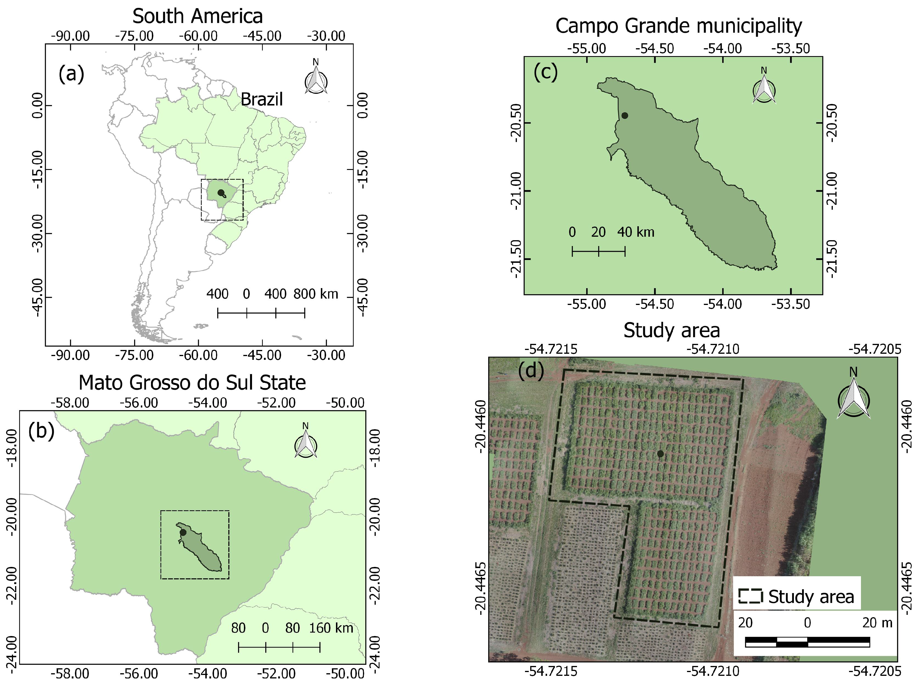
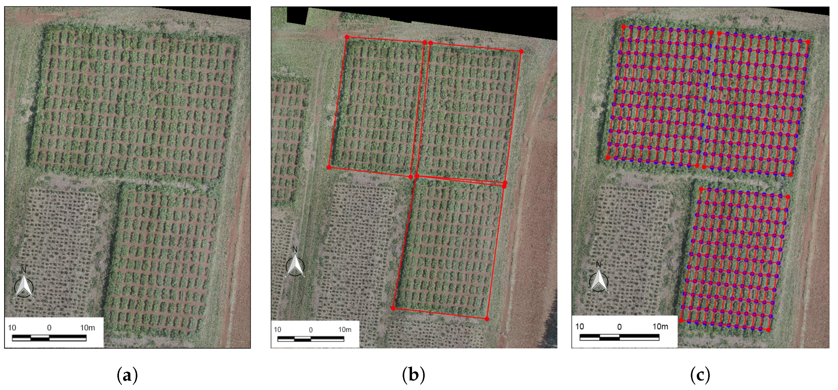
2.1. Study Area and Dataset
2.2. Deep Learning Approach and Experimental Setup
3. Experimental Results Evaluation
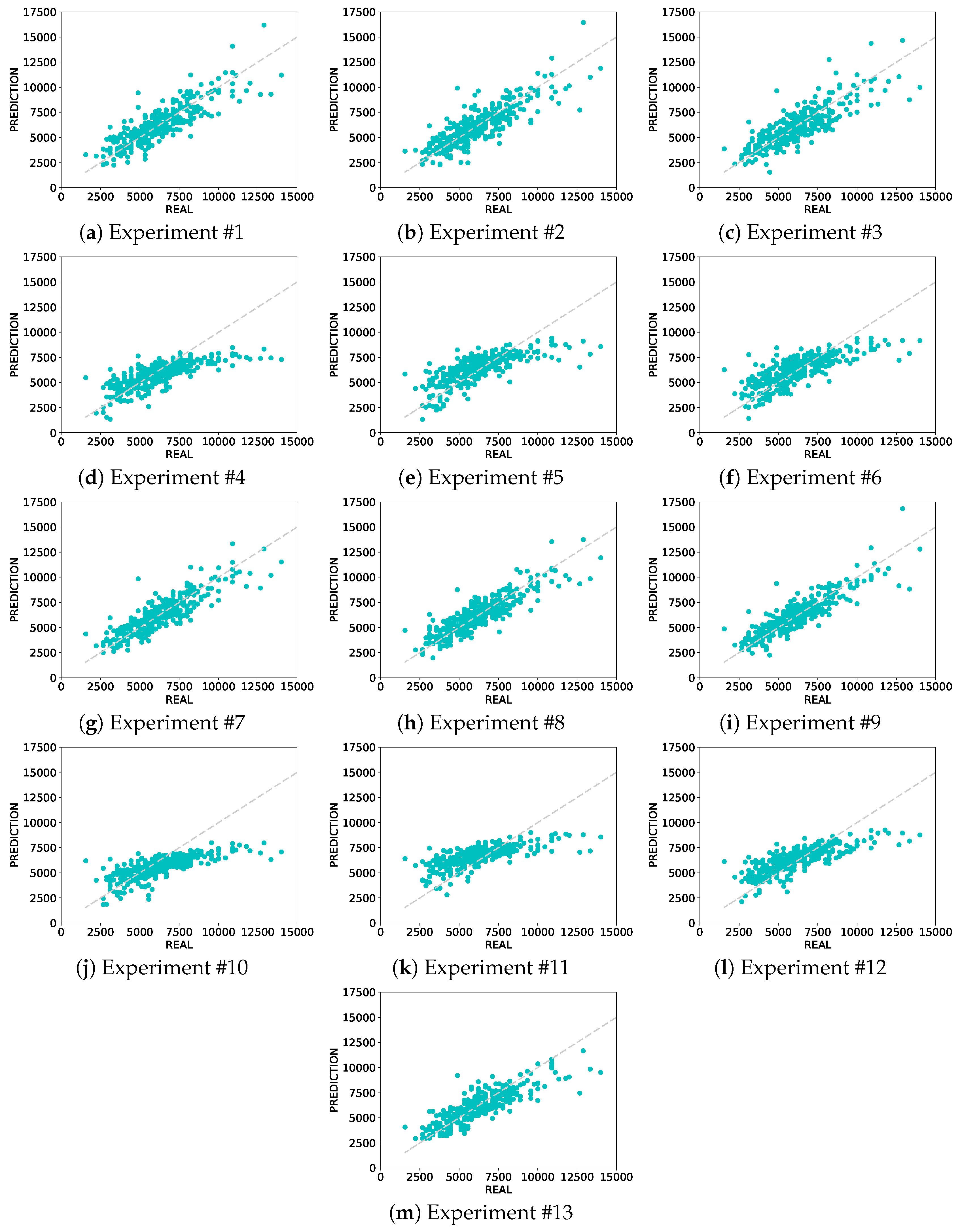
3.1. Standard Evaluation: MAE, MAPE, R, and Graph of Predicted Versus Real
3.2. ROC Regression
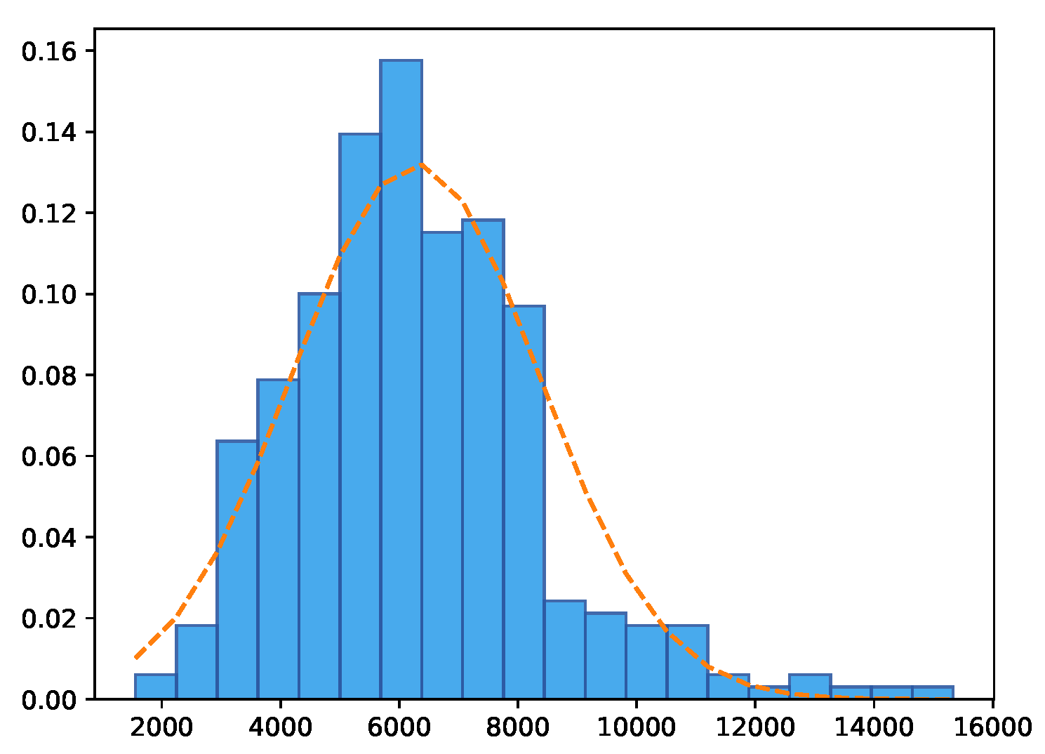
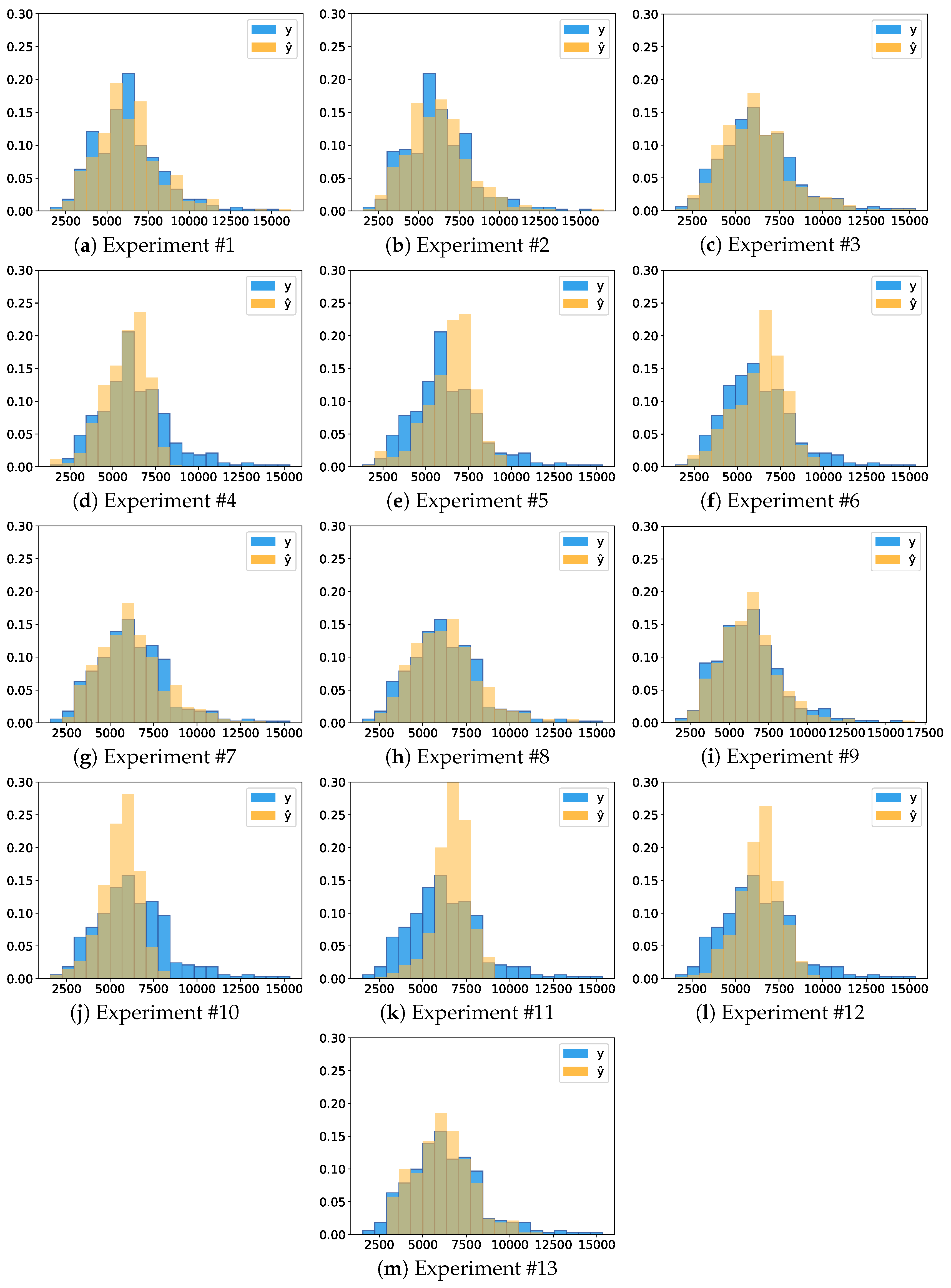
3.3. Histograms
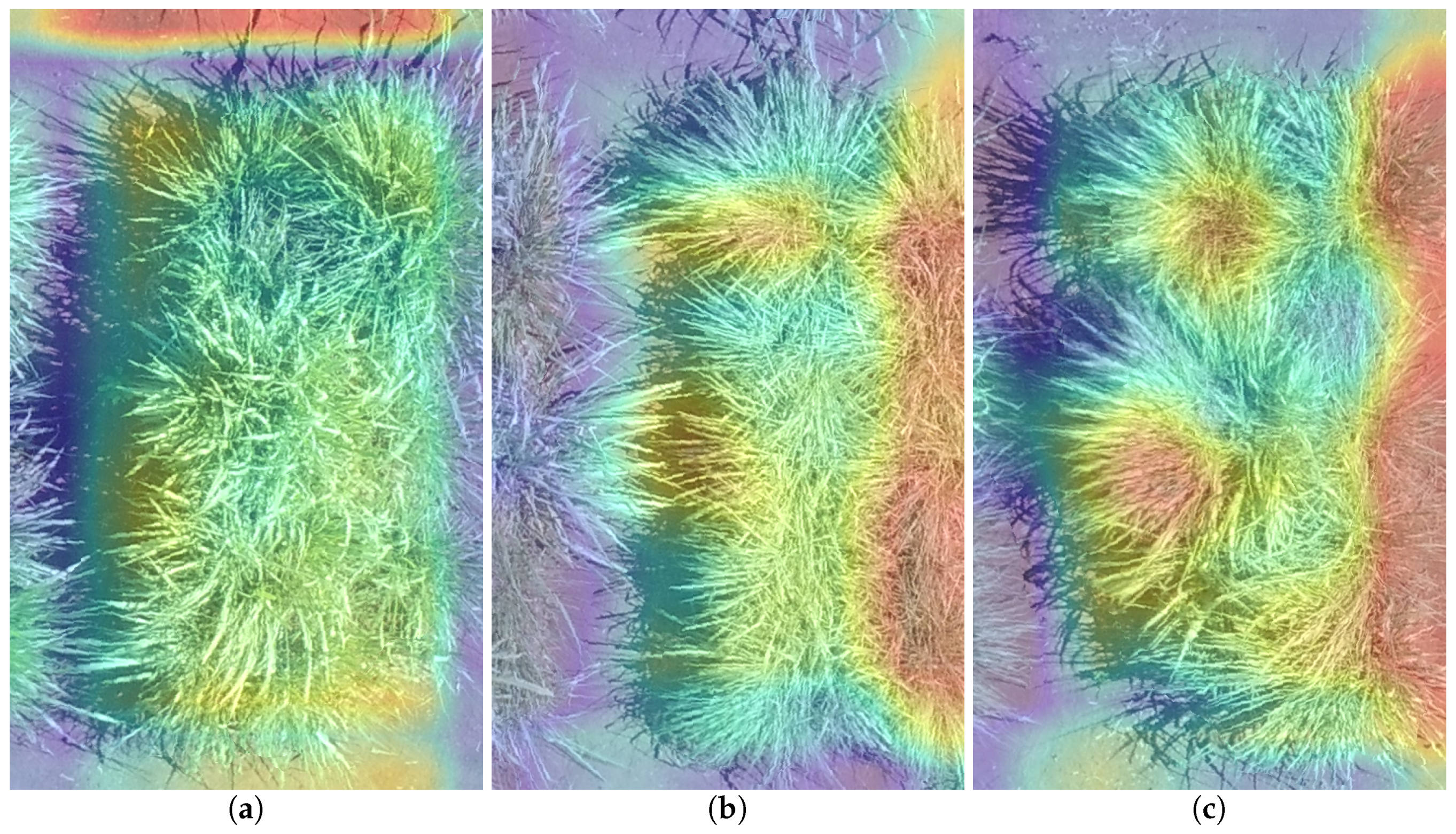
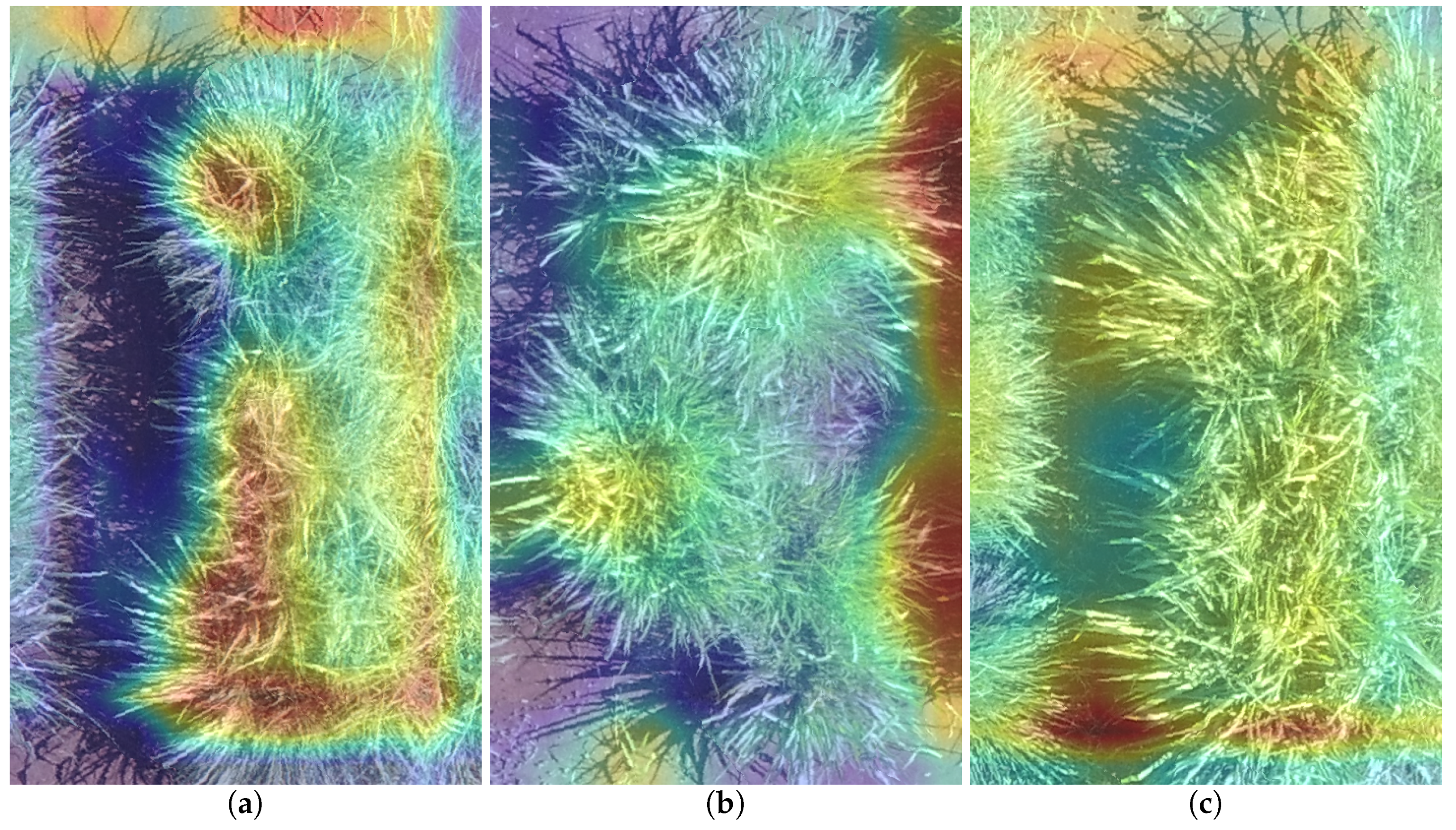
3.4. Visual Inspection
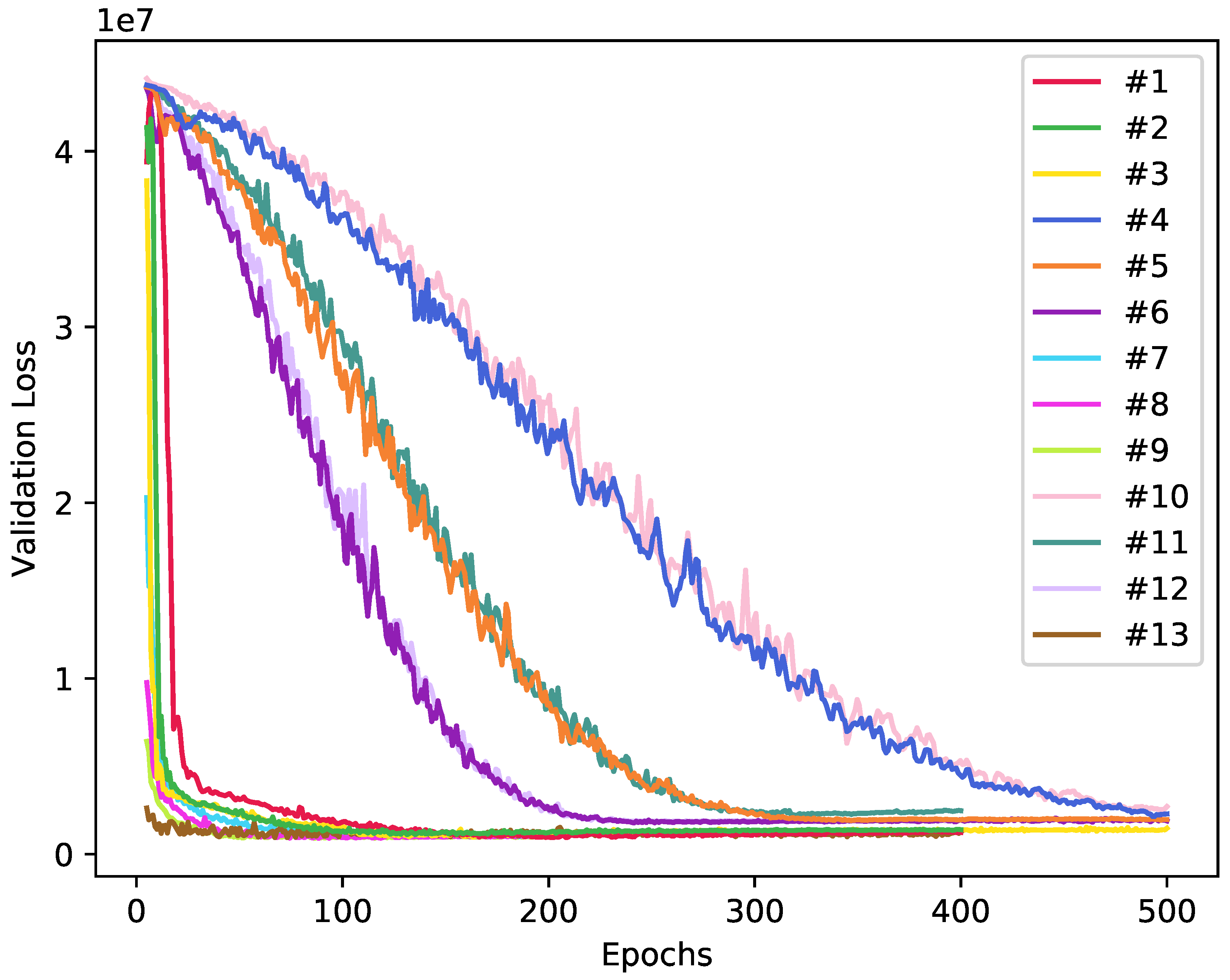
3.5. Training and Test Time
4. Discussion
5. Conclusions
Author Contributions
Funding
Acknowledgments
Conflicts of Interest
References
- Bendig, J.; Bolten, A.; Bennertz, S.; Broscheit, J.; Eichfuss, S.; Bareth, G. Estimating Biomass of Barley Using Crop Surface Models (CSMs) Derived from UAV-Based RGB Imaging. Remote Sens. 2014, 6, 10395–10412. [Google Scholar] [CrossRef] [Green Version]
- Gebremedhin, A.; Badenhorst, P.E.; Wang, J.; Spangenberg, G.C.; Smith, K.F. Prospects for measurement of dry matter yield in forage breeding programs using sensor technologies. Agronomy 2019, 9, 65. [Google Scholar] [CrossRef] [Green Version]
- Weiss, M.; Jacob, F.; Duveiller, G. Remote sensing for agricultural applications: A meta-review. Remote Sens. Environ. 2020, 236, 111402. [Google Scholar] [CrossRef]
- Osco, L.P.; Ramos, A.P.M.; Pereira, D.R.; Moriya, É.A.S.; Imai, N.N.; Matsubara, E.T.; Estrabis, N.; de Souza, M.; Junior, J.M.; Gonçalves, W.N.; et al. Predicting canopy nitrogen content in citrus-trees using random forest algorithm associated to spectral vegetation indices from UAV-imagery. Remote Sens. 2019, 11, 2925. [Google Scholar] [CrossRef] [Green Version]
- D’Oliveira, M.V.N.; Broadbent, E.N.; Oliveira, L.C.; Almeida, D.R.A.; Papa, D.A.; Ferreira, M.E.; Zambrano, A.M.A.; Silva, C.A.; Avino, F.S.; Prata, G.A.; et al. Aboveground Biomass Estimation in Amazonian Tropical Forests: A Comparison of Aircraft- and GatorEye UAV-borne LiDAR Data in the Chico Mendes Extractive Reserve in Acre, Brazil. Remote Sens. 2020, 12, 1754. [Google Scholar] [CrossRef]
- Miyoshi, G.T.; Arruda, M.D.S.; Osco, L.P.; Junior, J.M.; Gonçalves, D.N.; Imai, N.N.; Tommaselli, A.M.G.; Honkavaara, E.; Gonçalves, W.N. A novel deep learning method to identify single tree species in UAV-based hyperspectral images. Remote Sens. 2020, 12, 1294. [Google Scholar] [CrossRef] [Green Version]
- Leiva, J.N.; Robbins, J.; Saraswat, D.; She, Y.; Ehsani, R. Evaluating remotely sensed plant count accuracy with differing unmanned aircraft system altitudes, physical canopy separations, and ground covers. J. Appl. Remote Sens. 2017, 11, 036003. [Google Scholar] [CrossRef]
- Liu, T.; Abd-Elrahman, A.; Morton, J.; Wilhelm, V.L. Comparing fully convolutional networks, random forest, support vector machine, and patch-based deep convolutional neural networks for object-based wetland mapping using images from small unmanned aircraft system. GISci. Remote Sens. 2018, 55, 243–264. [Google Scholar] [CrossRef]
- Abdulridha, J.; Batuman, O.; Ampatzidis, Y. UAV-based remote sensing technique to detect citrus canker disease utilizing hyperspectral imaging and machine learning. Remote Sens. 2019, 11. [Google Scholar] [CrossRef] [Green Version]
- Feng, P.; Wang, B.; Liu, D.L.; Yu, Q. Machine learning-based integration of remotely-sensed drought factors can improve the estimation of agricultural drought in South-Eastern Australia. Agric. Syst. 2019, 173, 303–316. [Google Scholar] [CrossRef]
- Osco, L.P.; Ramos, A.P.M.; Pinheiro, M.M.F.; Moriya, É.A.S.; Imai, N.N.; Estrabis, N.; Ianczyk, F.; de Araújo, F.F.; Liesenberg, V.; de Castro Jorge, L.A.; et al. A machine learning framework to predict nutrient content in valencia-orange leaf hyperspectral measurements. Remote Sens. 2020, 12, 906. [Google Scholar] [CrossRef] [Green Version]
- Ghamisi, P.; Plaza, J.; Chen, Y.; Li, J.; Plaza, A.J. Advanced Spectral Classifiers for Hyperspectral Images: A review. IEEE Geosci. Remote Sens. Mag. 2017, 5, 8–32. [Google Scholar] [CrossRef] [Green Version]
- Al-Saffar, A.A.M.; Tao, H.; Talab, M.A. Review of deep convolution neural network in image classification. In Proceedings of the 2017 International Conference on Radar, Antenna, Microwave, Electronics, and Telecommunications (ICRAMET), Jakarta, Indonesia, 23–24 October 2017; pp. 26–31. [Google Scholar]
- Alshehhi, R.; Marpu, P.R.; Woon, W.L.; Mura, M.D. Simultaneous extraction of roads and buildings in remote sensing imagery with convolutional neural networks. ISPRS J. Photogramm. Remote Sens. 2017, 130, 139–149. [Google Scholar] [CrossRef]
- Khamparia, A.; Singh, K.M. A systematic review on deep learning architectures and applications. Expert Syst. 2019, 36, 1–22. [Google Scholar] [CrossRef]
- Csillik, O.; Cherbini, J.; Johnson, R.; Lyons, A.; Kelly, M. Identification of Citrus Trees from Unmanned Aerial Vehicle Imagery Using Convolutional Neural Networks. Drones 2018, 2, 39. [Google Scholar] [CrossRef] [Green Version]
- Hassanein, M.; Khedr, M.; El-Sheimy, N. Crop row detection procedure using low-cost uav imagery system. Int. Arch. Photogramm. Remote Sens. Spat. Inf. Sci. 2019, 42, 349–356. [Google Scholar] [CrossRef] [Green Version]
- Wu, L.; Zhu, X.; Lawes, R.; Dunkerley, D.; Zhang, H. Comparison of machine learning algorithms for classification of LiDAR points for characterization of canola canopy structure. Int. J. Remote Sens. 2019, 40, 5973–5991. [Google Scholar] [CrossRef]
- Kitano, B.T.; Mendes, C.C.T.; Geus, A.R.; Oliveira, H.C.; Souza, J.R. Corn Plant Counting Using Deep Learning and UAV Images. IEEE Geosci. Remote Sens. Lett. 2019, 1–5. [Google Scholar] [CrossRef]
- Dian Bah, M.; Hafiane, A.; Canals, R. Deep learning with unsupervised data labeling for weed detection in line crops in UAV images. Remote Sens. 2018, 10, 1690. [Google Scholar] [CrossRef] [Green Version]
- Legg, M.; Bradley, S. Ultrasonic Arrays for Remote Sensing of Pasture Biomass. Remote Sens. 2019, 12, 111. [Google Scholar] [CrossRef] [Green Version]
- Loggenberg, K.; Strever, A.; Greyling, B.; Poona, N. Modelling water stress in a Shiraz vineyard using hyperspectral imaging and machine learning. Remote Sens. 2018, 10, 202. [Google Scholar] [CrossRef] [Green Version]
- Fan, Z.; Lu, J.; Gong, M.; Xie, H.; Goodman, E.D. Automatic Tobacco Plant Detection in UAV Images via Deep Neural Networks. IEEE J. Sel. Top. Appl. Earth Obs. Remote Sens. 2018, 11, 876–887. [Google Scholar] [CrossRef]
- Bendig, J.; Yu, K.; Aasen, H.; Bolten, A.; Bennertz, S.; Broscheit, J.; Gnyp, M.L.; Bareth, G. Combining UAV-based plant height from crop surface models, visible, and near infrared vegetation indices for biomass monitoring in barley. Int. J. Appl. Earth Obs. Geoinf. 2015, 39, 79–87. [Google Scholar] [CrossRef]
- Ballesteros, R.; Ortega, J.F.; Hernandez, D.; Moreno, M.A. Onion biomass monitoring using UAV-based RGB imaging. Precis. Agric. 2018, 19, 840–857. [Google Scholar] [CrossRef]
- Batistoti, J.; Marcato Junior, J.; Ítavo, L.; Matsubara, E.; Gomes, E.; Oliveira, B.; Souza, M.; Siqueira, H.; Salgado Filho, G.; Akiyama, T.; et al. Estimating Pasture Biomass and Canopy Height in Brazilian Savanna Using UAV Photogrammetry. Remote Sens. 2019, 11, 2447. [Google Scholar] [CrossRef] [Green Version]
- Näsi, R.; Viljanen, N.; Kaivosoja, J.; Alhonoja, K.; Hakala, T.; Markelin, L.; Honkavaara, E. Estimating Biomass and Nitrogen Amount of Barley and Grass Using UAV and Aircraft Based Spectral and Photogrammetric 3D Features. Remote Sens. 2018, 10, 1082. [Google Scholar] [CrossRef] [Green Version]
- Li, B.; Xu, X.; Zhang, L.; Han, J.; Bian, C.; Li, G.; Liu, J.; Jin, L. Above-ground biomass estimation and yield prediction in potato by using UAV-based RGB and hyperspectral imaging. ISPRS J. Photogramm. Remote Sens. 2020, 162, 161–172. [Google Scholar] [CrossRef]
- Kamilaris, A.; Prenafeta-Boldú, F.X. Deep learning in agriculture: A survey. Comput. Electron. Agric. 2018, 147, 70–90. [Google Scholar] [CrossRef] [Green Version]
- Ma, J.; Li, Y.; Chen, Y.; Du, K.; Zheng, F.; Zhang, L.; Sun, Z. Estimating above ground biomass of winter wheat at early growth stages using digital images and deep convolutional neural network. Eur. J. Agron. 2019, 103, 117–129. [Google Scholar] [CrossRef]
- Jank, L.; Barrios, S.C.; do Valle, C.B.; Simeão, R.M.; Alves, G.F. The value of improved pastures to Brazilian beef production. Crop Pasture Sci. 2014, 65, 1132–1137. [Google Scholar] [CrossRef]
- Hunter, J.D. Matplotlib: A 2D graphics environment. Comput. Sci. Eng. 2007, 9, 90–95. [Google Scholar] [CrossRef]
- Gillies, S.; Ward, B.; Petersen, A.S. Rasterio: Geospatial Raster I/O for Python Programmers. 2013. Available online: https://github.com/mapbox/rasterio (accessed on 17 August 2020).
- Oliphant, T.E. Python for scientific computing. Comput. Sci. Eng. 2007, 9, 10–20. [Google Scholar] [CrossRef] [Green Version]
- LeCun, Y.; Bengio, Y.; Hinton, G. Deep learning. Nature 2015, 521, 436–444. [Google Scholar] [CrossRef] [PubMed]
- Lu, J.; Behbood, V.; Hao, P.; Zuo, H.; Xue, S.; Zhang, G. Transfer learning using computational intelligence: A survey. Knowl.-Based Syst. 2015, 80, 14–23. [Google Scholar] [CrossRef]
- Zhang, C.; Bengio, S.; Hardt, M.; Recht, B.; Vinyals, O. Understanding deep learning requires rethinking generalization. arXiv 2016, arXiv:1611.03530. [Google Scholar]
- Shorten, C.; Khoshgoftaar, T.M. A survey on image data augmentation for deep learning. J. Big Data 2019, 6, 60. [Google Scholar] [CrossRef]
- Krizhevsky, A.; Sutskever, I.; Hinton, G.E. Imagenet Classification with Deep Convolutional Neural Networks. 2012. Available online: http://papers.nips.cc/paper/4824-imagenet-classification-with-deep-convolutional-neural-networ (accessed on 10 August 2020).
- He, K.; Zhang, X.; Ren, S.; Sun, J. Deep residual learning for image recognition. In Proceedings of the IEEE Conference on Computer Vision and Pattern Recognition, Las Vegas, NV, USA, 27–30 June 2016; pp. 770–778. [Google Scholar]
- Simonyan, K.; Zisserman, A. Very Deep Convolutional Networks for Large-Scale Image Recognition. arXiv 2014, arXiv:1409.1556. [Google Scholar]
- Paszke, A.; Gross, S.; Massa, F.; Lerer, A.; Bradbury, J.; Chanan, G.; Killeen, T.; Lin, Z.; Gimelshein, N.; Antiga, L.; et al. PyTorch: An imperative style, high-performance deep learning library. In Proceedings of the Advances in Neural Information Processing Systems, Vancouver, BC, Canada, 8–14 December 2019; pp. 8024–8035. [Google Scholar]
- Kingma, D.P.; Ba, J. Adam: A method for stochastic optimization. arXiv 2014, arXiv:1412.6980. [Google Scholar]
- Weiss, S.M.; Kapouleas, I. An empirical comparison of pattern recognition, neural nets, and machine learning classification methods. IJCAI 1989, 89, 781–787. [Google Scholar]
- Blum, A.; Kalai, A.; Langford, J. Beating the hold-out: Bounds for k-fold and progressive cross-validation. In Proceedings of the Twelfth Annual Conference on Computational Learning Theory, Santa Cruz, CA, USA, 7–9 July 1999; pp. 203–208. [Google Scholar]
- Hernández-Orallo, J. ROC curves for regression. Pattern Recognit. 2013, 46, 3395–3411. [Google Scholar] [CrossRef] [Green Version]
- Thorndike, R.L. Who belongs in the family. Psychometrika 1953, 18, 267–276. [Google Scholar] [CrossRef]
- Zhou, B.; Khosla, A.; Lapedriza, A.; Oliva, A.; Torralba, A. Learning deep features for discriminative localization. In Proceedings of the IEEE Conference on Computer Vision and Pattern Recognition, Las Vegas, NV, USA, 27–30 June 2016; pp. 2921–2929. [Google Scholar]
- Selvaraju, R.R.; Cogswell, M.; Das, A.; Vedantam, R.; Parikh, D.; Batra, D. Grad-cam: Visual explanations from deep networks via gradient-based localization. In Proceedings of the IEEE International Conference on Computer Vision, Venice, Italy, 22–29 October 2017; pp. 618–626. [Google Scholar]
- Viljanen, N.; Honkavaara, E.; Näsi, R.; Hakala, T.; Niemeläinen, O.; Kaivosoja, J. A novel machine learning method for estimating biomass of grass swards using a photogrammetric canopy height model, images and vegetation indices captured by a drone. Agriculture 2018, 8, 70. [Google Scholar] [CrossRef] [Green Version]
- Moeckel, T.; Safari, H.; Reddersen, B.; Fricke, T.; Wachendorf, M. Fusion of ultrasonic and spectral sensor data for improving the estimation of biomass in grasslands with heterogeneous sward structure. Remote Sens. 2017, 9, 98. [Google Scholar] [CrossRef] [Green Version]
- Wachendorf, M.; Fricke, T.; Möckel, T. Remote sensing as a tool to assess botanical composition, structure, quantity and quality of temperate grasslands. Grass Forage Sci. 2018, 73, 1–14. [Google Scholar] [CrossRef]
- Marabel, M.; Alvarez-Taboada, F. Spectroscopic determination of aboveground biomass in grasslands using spectral transformations, support vector machine and partial least squares regression. Sensors 2013, 13, 10027–10051. [Google Scholar] [CrossRef] [PubMed] [Green Version]


| #Experiment | Model | Batch Size | Data-Set | Epochs |
|---|---|---|---|---|
| 1 | AlexNet | 256 | original | 400 |
| 2 | AlexNet | 256 | augmented h | 400 |
| 3 | AlexNet | 256 | augmented hv | 500 |
| 4 | Resnet18 | 128 | original | 500 |
| 5 | Resnet18 | 128 | augmented h | 500 |
| 6 | Resnet18 | 128 | augmented hv | 500 |
| 7 | AlexNet Pre-Trained | 256 | original | 200 |
| 8 | AlexNet Pre-Trained | 256 | augmented h | 200 |
| 9 | AlexNet Pre-Trained | 256 | augmented hv | 200 |
| 10 | ResNet18 Pre-Trained | 128 | original | 500 |
| 11 | ResNet18 Pre-Trained | 128 | augmented h | 400 |
| 12 | ResNet18 Pre-Trained | 128 | augmented hv | 400 |
| 13 | VGGNet11 Pre-Trained | 64 | augmented hv | 400 |
| #Experiment | Model | Mean Absolute Error | Mean Absolute Percentage Error | Correlation (r) |
|---|---|---|---|---|
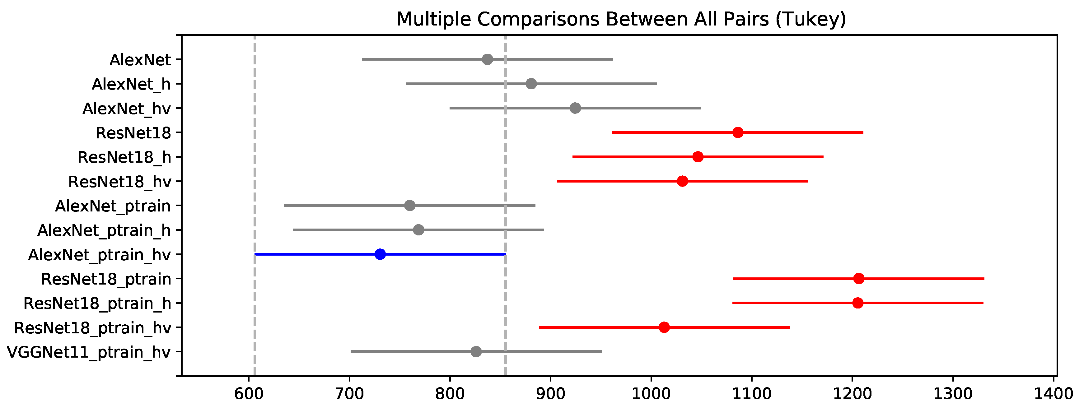
| 1 | AlexNet | 837 ± 106 | 14.58 ± 2.52 | 0.84 ± 0.03 |
| 2 | AlexNet h | 880 ± 202 | 15.11 ± 3.24 | 0.83 ± 0.06 |
| 3 | AlexNet hv | 924 ± 143 | 15.48 ± 2.30 | 0.82 ± 0.05 |
| 4 | ResNet18 | 1086 ± 219 | 17.70 ± 3.41 | 0.74 ± 0.06 |
| 5 | ResNet18 h | 1046 ± 107 | 19.01 ± 2.77 | 0.74 ± 0.06 |
| 6 | ResNet18 hv | 1031 ± 153 | 18.76 ± 4.28 | 0.75 ± 0.06 |
| 7 | AlexNet Pre-Trained | 759 ± 102 | 13.23 ± 2.23 | 0.87 ± 0.05 |
| 8 | AlexNet Pre-Trained h | 768 ± 123 | 13.54 ± 2.88 | 0.87 ± 0.03 |
| 9 | AlexNet Pre-Trained hv | 730 ± 59 | 12.98 ± 2.18 | 0.88 ± 0.04 |
| 10 | ResNet18 Pre-Trained | 1206 ± 233 | 19.46 ± 5.15 | 0.73 ± 0.04 |
| 11 | ResNet18 Pre-Trained h | 1205 ± 194 | 23.16 ± 4.80 | 0.71 ± 0.07 |
| 12 | ResNet18 Pre-Trained hv | 1012 ± 128 | 18.58 ± 2.34 | 0.77 ± 0.05 |
| 13 | VGGNet11 Pre-Trained | 825 ± 152 | 13.89 ± 3.09 | 0.84 ± 0.04 |
| Experiment | 1 | 2 | 3 | 4 | 5 | 6 | 7 | 8 | 9 | 10 | 11 | 12 | 13 |
| Intersection Area | 0.83 | 0.83 | 0.91 | 0.78 | 0.72 | 0.78 | 0.89 | 0.89 | 0.92 | 0.68 | 0.62 | 0.76 | 0.90 |
| #Experiment | Model | Training Time (min) | Test Time (s) |
|---|---|---|---|
| 1 | AlexNet | 35.8 | 0.39 |
| 2 | AlexNet h | 95.6 | 0.46 |
| 3 | AlexNet hv | 122.2 | 0.40 |
| 4 | ResNet18 | 60.2 | 0.47 |
| 5 | ResNet18 h | 131.3 | 0.54 |
| 6 | ResNet18 hv | 133.7 | 0.53 |
| 7 | AlexNet Pre-Trained | 15.8 | 0.37 |
| 8 | AlexNet Pre-Trained h | 36.2 | 0.44 |
| 9 | AlexNet Pre-Trained hv | 43.7 | 0.50 |
| 10 | ResNet18 Pre-Trained | 58.1 | 0.47 |
| 11 | ResNet18 Pre-Trained h | 102.2 | 0.67 |
| 12 | ResNet18 Pre-Trained hv | 104.4 | 0.43 |
| 13 | VGGNet11 Pre-Trained hv | 372.2 | 0.81 |
© 2020 by the authors. Licensee MDPI, Basel, Switzerland. This article is an open access article distributed under the terms and conditions of the Creative Commons Attribution (CC BY) license (http://creativecommons.org/licenses/by/4.0/).
Share and Cite
Castro, W.; Marcato Junior, J.; Polidoro, C.; Osco, L.P.; Gonçalves, W.; Rodrigues, L.; Santos, M.; Jank, L.; Barrios, S.; Valle, C.; et al. Deep Learning Applied to Phenotyping of Biomass in Forages with UAV-Based RGB Imagery. Sensors 2020, 20, 4802. https://doi.org/10.3390/s20174802
Castro W, Marcato Junior J, Polidoro C, Osco LP, Gonçalves W, Rodrigues L, Santos M, Jank L, Barrios S, Valle C, et al. Deep Learning Applied to Phenotyping of Biomass in Forages with UAV-Based RGB Imagery. Sensors. 2020; 20(17):4802. https://doi.org/10.3390/s20174802
Chicago/Turabian StyleCastro, Wellington, José Marcato Junior, Caio Polidoro, Lucas Prado Osco, Wesley Gonçalves, Lucas Rodrigues, Mateus Santos, Liana Jank, Sanzio Barrios, Cacilda Valle, and et al. 2020. "Deep Learning Applied to Phenotyping of Biomass in Forages with UAV-Based RGB Imagery" Sensors 20, no. 17: 4802. https://doi.org/10.3390/s20174802