Figure 1.
Lower Limb Robotic Rehabilitation Exoskeleton.
Figure 1.
Lower Limb Robotic Rehabilitation Exoskeleton.
Figure 2.
Reference trajectories of the hip and knee joints.
Figure 2.
Reference trajectories of the hip and knee joints.
Figure 3.
Topology of proposed active disturbance rejection control (ADRC) for lower limb robotic rehabilitation exoskeleton (LLRRE).
Figure 3.
Topology of proposed active disturbance rejection control (ADRC) for lower limb robotic rehabilitation exoskeleton (LLRRE).
Figure 4.
Gait trajectory tracking comparison of ADRC, ADRC-NLSEF, ADRC-TD, and ADRC-NLSEF-TD for the hip joint with a reference without disturbance.
Figure 4.
Gait trajectory tracking comparison of ADRC, ADRC-NLSEF, ADRC-TD, and ADRC-NLSEF-TD for the hip joint with a reference without disturbance.
Figure 5.
Gait trajectory tracking comparison of ADRC, ADRC-NLSEF, ADRC-TD, and ADRC-NLSEF-TD for the knee joint with a reference without disturbance.
Figure 5.
Gait trajectory tracking comparison of ADRC, ADRC-NLSEF, ADRC-TD, and ADRC-NLSEF-TD for the knee joint with a reference without disturbance.
Figure 6.
Control signal trajectory tracking comparison of ADRC, ADRC-NLSEF, ADRC-TD, and ADRC-NLSEF-TD for the hip joint with no disturbance. (a) initial response of the control signal; (b) control signal in blown up.
Figure 6.
Control signal trajectory tracking comparison of ADRC, ADRC-NLSEF, ADRC-TD, and ADRC-NLSEF-TD for the hip joint with no disturbance. (a) initial response of the control signal; (b) control signal in blown up.
Figure 7.
Control signal trajectory tracking comparison of ADRC, ADRC-NLSEF, ADRC-TD, and ADRC-NLSEF-TD for the knee joint with no disturbance.
Figure 7.
Control signal trajectory tracking comparison of ADRC, ADRC-NLSEF, ADRC-TD, and ADRC-NLSEF-TD for the knee joint with no disturbance.
Figure 8.
Gait trajectory tracking error comparison of ADRC, ADRC-NLSEF, ADRC-TD, and ADRC-NLSEF-TD for the hip joint with a reference without disturbance.
Figure 8.
Gait trajectory tracking error comparison of ADRC, ADRC-NLSEF, ADRC-TD, and ADRC-NLSEF-TD for the hip joint with a reference without disturbance.
Figure 9.
Gait trajectory tracking error comparison of ADRC, ADRC-NLSEF, ADRC-TD, and ADRC-NLSEF-TD for the knee joint with a reference without disturbance.
Figure 9.
Gait trajectory tracking error comparison of ADRC, ADRC-NLSEF, ADRC-TD, and ADRC-NLSEF-TD for the knee joint with a reference without disturbance.
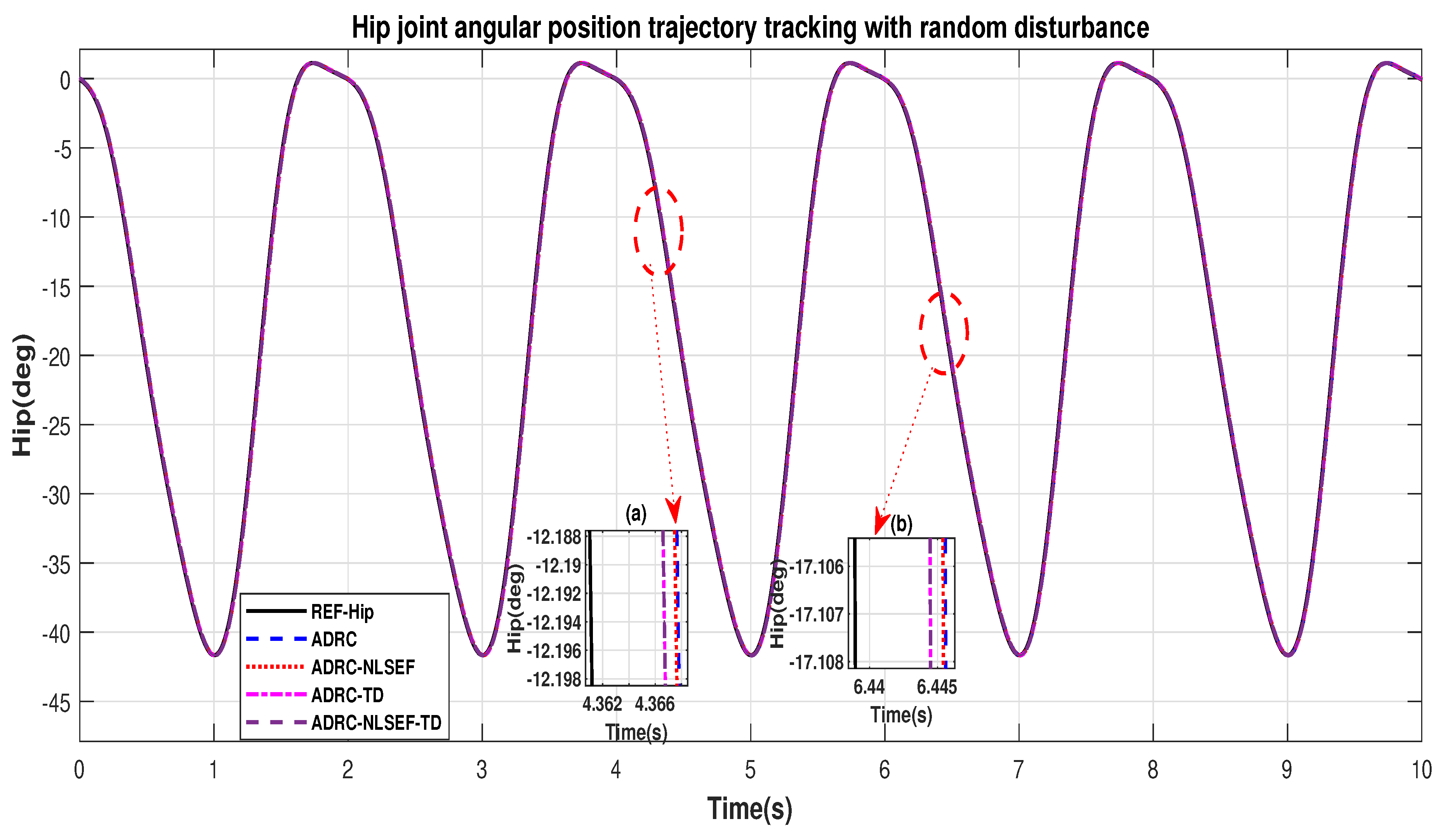
Figure 10.
Gait trajectory tracking comparison of ADRC, ADRC-NLSEF, ADRC-TD, and ADRC-NLSEF-TD for the hip joint with a reference with random disturbance.
Figure 10.
Gait trajectory tracking comparison of ADRC, ADRC-NLSEF, ADRC-TD, and ADRC-NLSEF-TD for the hip joint with a reference with random disturbance.
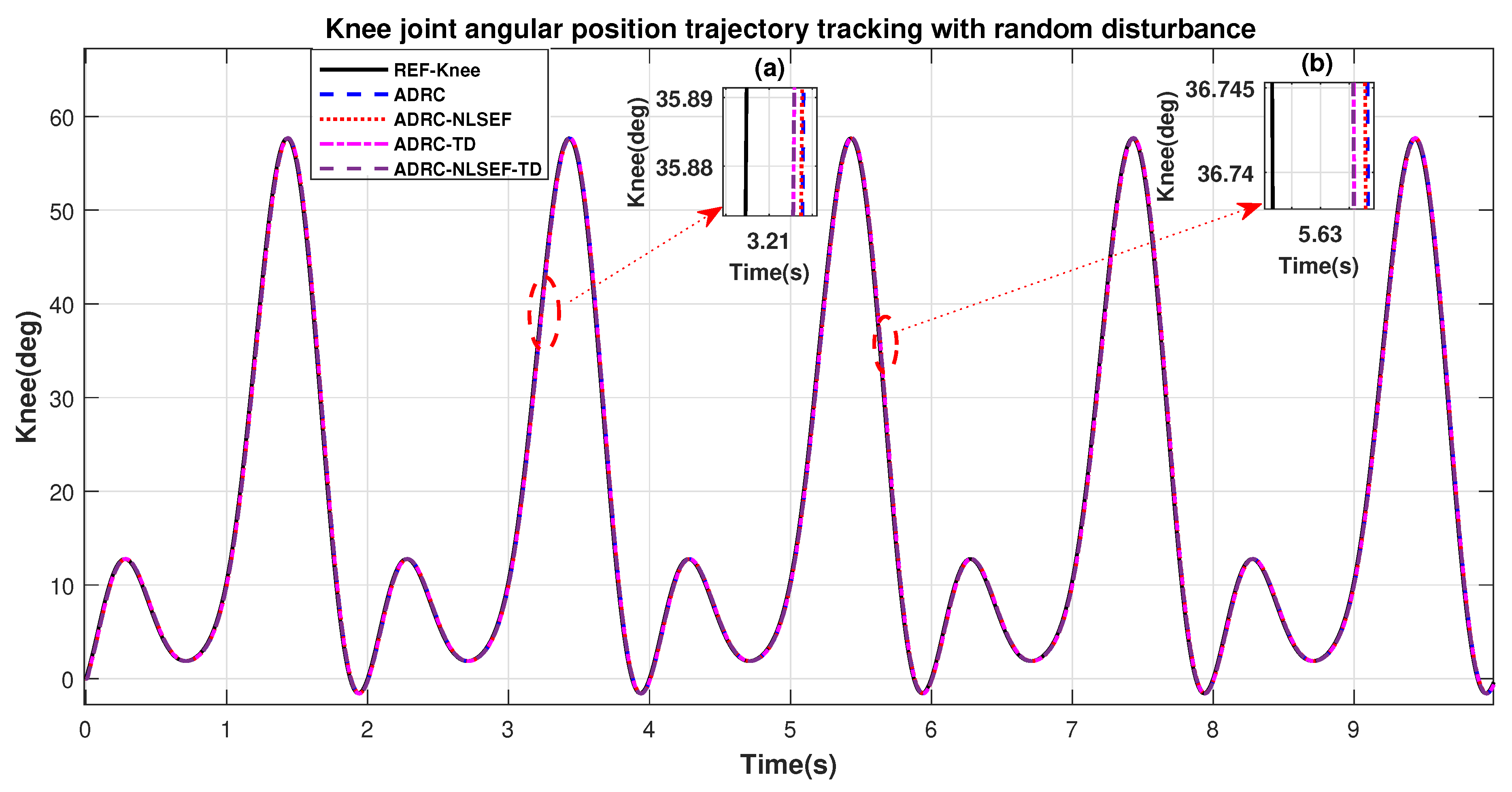
Figure 11.
Gait trajectory tracking comparison of ADRC, ADRC-NLSEF, ADRC-TD, and ADRC-NLSEF-TD for the knee joint with a reference with random disturbance.
Figure 11.
Gait trajectory tracking comparison of ADRC, ADRC-NLSEF, ADRC-TD, and ADRC-NLSEF-TD for the knee joint with a reference with random disturbance.
Figure 12.
Control signal trajectory tracking comparison of ADRC, ADRC-NLSEF, ADRC-TD, and ADRC-NLSEF-TD for the hip joint with random disturbance.
Figure 12.
Control signal trajectory tracking comparison of ADRC, ADRC-NLSEF, ADRC-TD, and ADRC-NLSEF-TD for the hip joint with random disturbance.
Figure 13.
Control signal trajectory tracking comparison of ADRC, ADRC-NLSEF, ADRC-TD, and ADRC-NLSEF-TD for the knee joint with random disturbance.
Figure 13.
Control signal trajectory tracking comparison of ADRC, ADRC-NLSEF, ADRC-TD, and ADRC-NLSEF-TD for the knee joint with random disturbance.
Figure 14.
Gait trajectory tracking error comparison of ADRC, ADRC-NLSEF, ADRC-TD, and ADRC-NLSEF-TD for the hip joint for reference signal with random disturbance.
Figure 14.
Gait trajectory tracking error comparison of ADRC, ADRC-NLSEF, ADRC-TD, and ADRC-NLSEF-TD for the hip joint for reference signal with random disturbance.
Figure 15.
Gait trajectory tracking error comparison of ADRC, ADRC-NLSEF, ADRC-TD, and ADRC-NLSEF-TD for the knee joint for reference signal with random disturbance.
Figure 15.
Gait trajectory tracking error comparison of ADRC, ADRC-NLSEF, ADRC-TD, and ADRC-NLSEF-TD for the knee joint for reference signal with random disturbance.
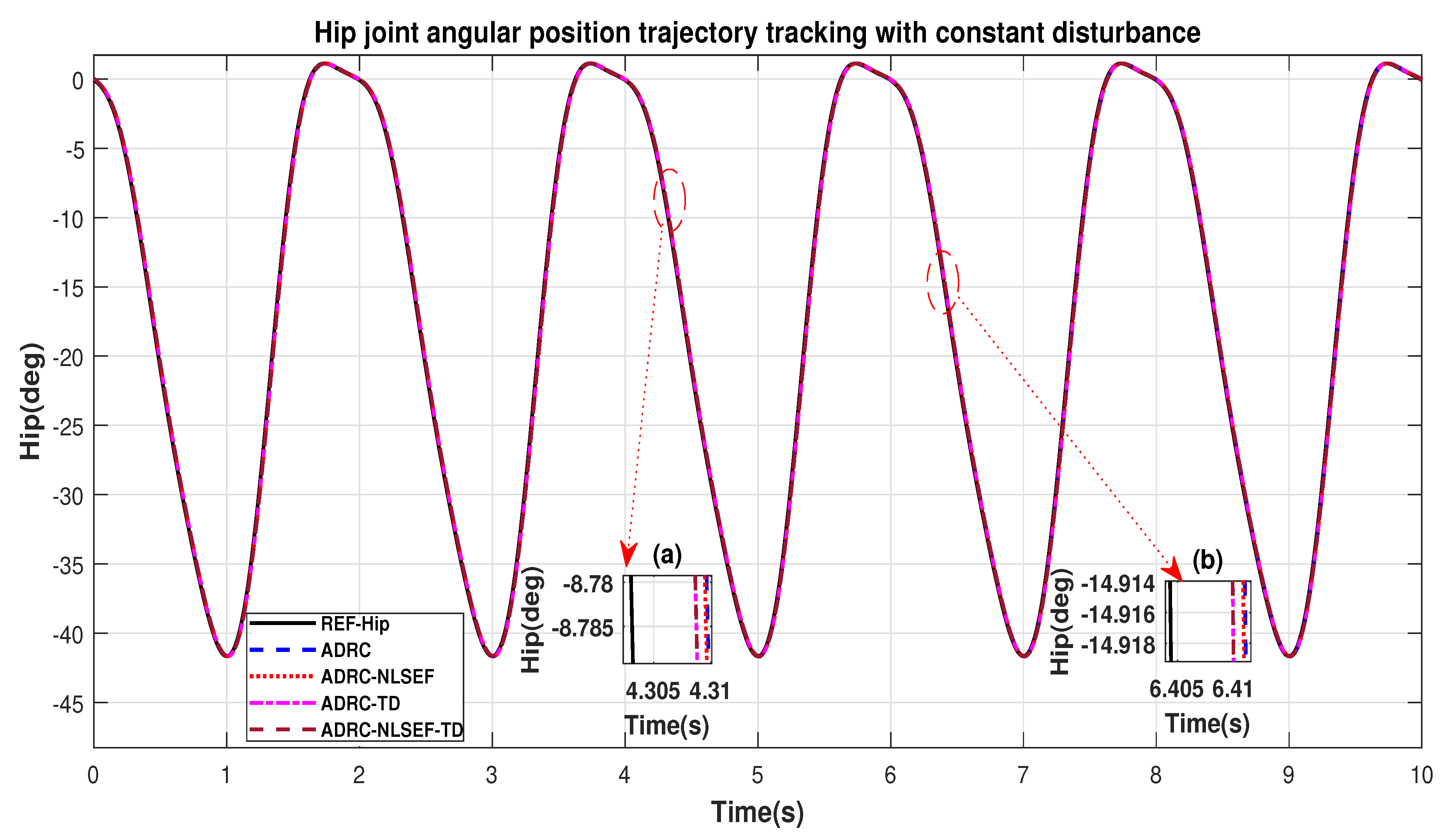
Figure 16.
Gait trajectory tracking comparison of ADRC, ADRC-NLSEF, ADRC-TD, and ADRC-NLSEF-TD for the hip joint with a reference with constant disturbance.
Figure 16.
Gait trajectory tracking comparison of ADRC, ADRC-NLSEF, ADRC-TD, and ADRC-NLSEF-TD for the hip joint with a reference with constant disturbance.
Figure 17.
Gait trajectory tracking comparison of ADRC, ADRC-NLSEF, ADRC-TD, and ADRC-NLSEF-TD for the knee joint with a reference with constant disturbance.
Figure 17.
Gait trajectory tracking comparison of ADRC, ADRC-NLSEF, ADRC-TD, and ADRC-NLSEF-TD for the knee joint with a reference with constant disturbance.
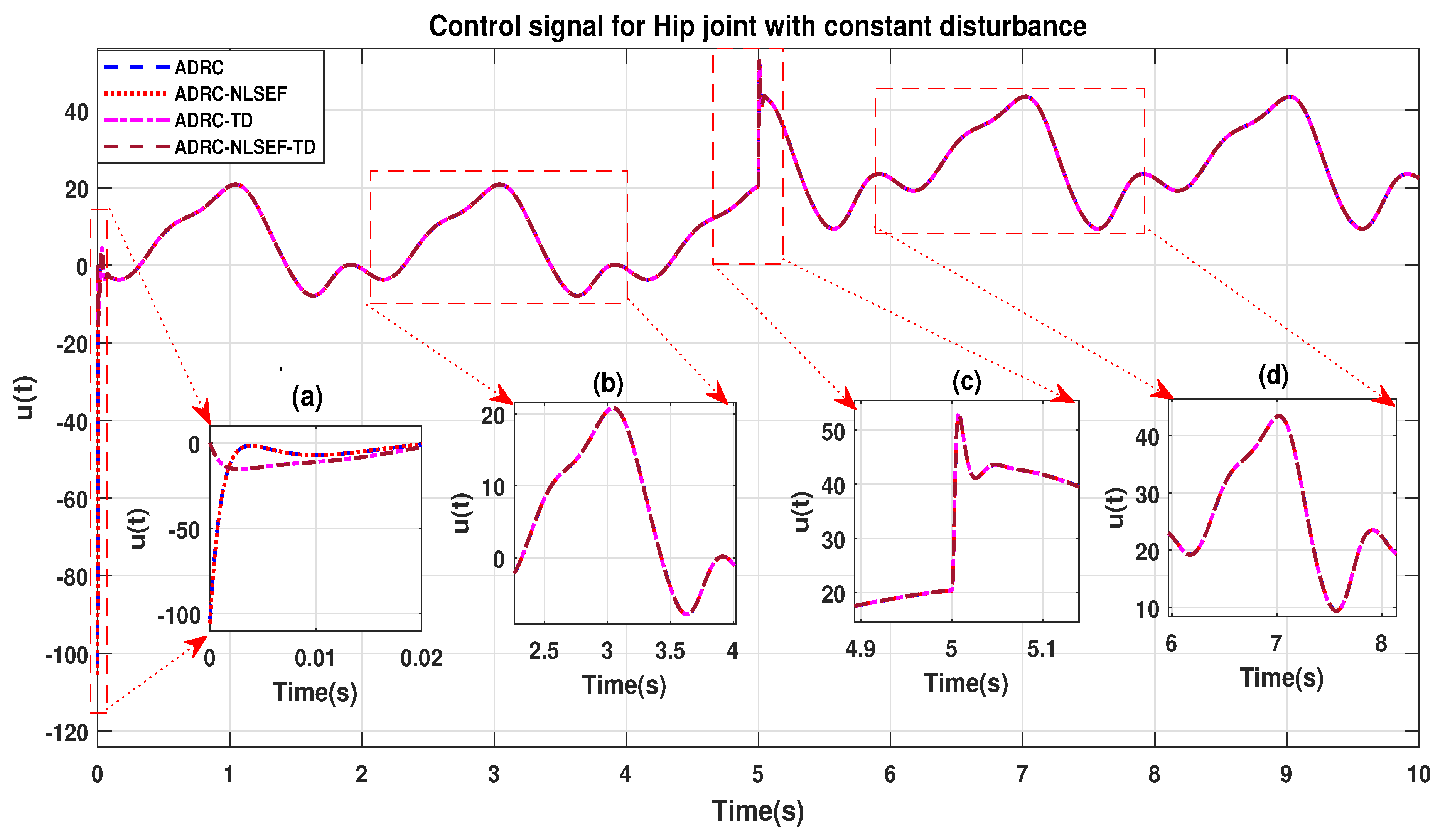
Figure 18.
Control signal comparison of ADRC, ADRC-NLSEF, ADRC-TD, and ADRC-NLSEF-TD for the hip joint with constant disturbance.
Figure 18.
Control signal comparison of ADRC, ADRC-NLSEF, ADRC-TD, and ADRC-NLSEF-TD for the hip joint with constant disturbance.
Figure 19.
Control signal comparison of ADRC, ADRC-NLSEF, ADRC-TD, and ADRC-NLSEF-TD for knee Joint with constant disturbance.
Figure 19.
Control signal comparison of ADRC, ADRC-NLSEF, ADRC-TD, and ADRC-NLSEF-TD for knee Joint with constant disturbance.
Figure 20.
Gait trajectory tracking error comparison of ADRC, ADRC-NLSEF, ADRC-TD, and ADRC-NLSEF-TD for the hip joint with a reference with constant disturbance.
Figure 20.
Gait trajectory tracking error comparison of ADRC, ADRC-NLSEF, ADRC-TD, and ADRC-NLSEF-TD for the hip joint with a reference with constant disturbance.
Figure 21.
Gait trajectory tracking error comparison of ADRC, ADRC-NLSEF, ADRC-TD, and ADRC-NLSEF-TD for knee joint with a reference with constant disturbance.
Figure 21.
Gait trajectory tracking error comparison of ADRC, ADRC-NLSEF, ADRC-TD, and ADRC-NLSEF-TD for knee joint with a reference with constant disturbance.
Figure 22.
Gait trajectory tracking comparison of ADRC, ADRC-NLSEF, ADRC-TD, and ADRC-NLSEF-TD for the hip joint with a reference with harmonic disturbance.
Figure 22.
Gait trajectory tracking comparison of ADRC, ADRC-NLSEF, ADRC-TD, and ADRC-NLSEF-TD for the hip joint with a reference with harmonic disturbance.
Figure 23.
Gait trajectory tracking comparison of ADRC, ADRC-NLSEF, ADRC-TD, and ADRC-NLSEF-TD for the knee joint with a reference with harmonic disturbance.
Figure 23.
Gait trajectory tracking comparison of ADRC, ADRC-NLSEF, ADRC-TD, and ADRC-NLSEF-TD for the knee joint with a reference with harmonic disturbance.
Figure 24.
Control signal comparison of ADRC, ADRC-NLSEF, ADRC-TD, and ADRC-NLSEF-TD for the hip joint with harmonic disturbance.
Figure 24.
Control signal comparison of ADRC, ADRC-NLSEF, ADRC-TD, and ADRC-NLSEF-TD for the hip joint with harmonic disturbance.
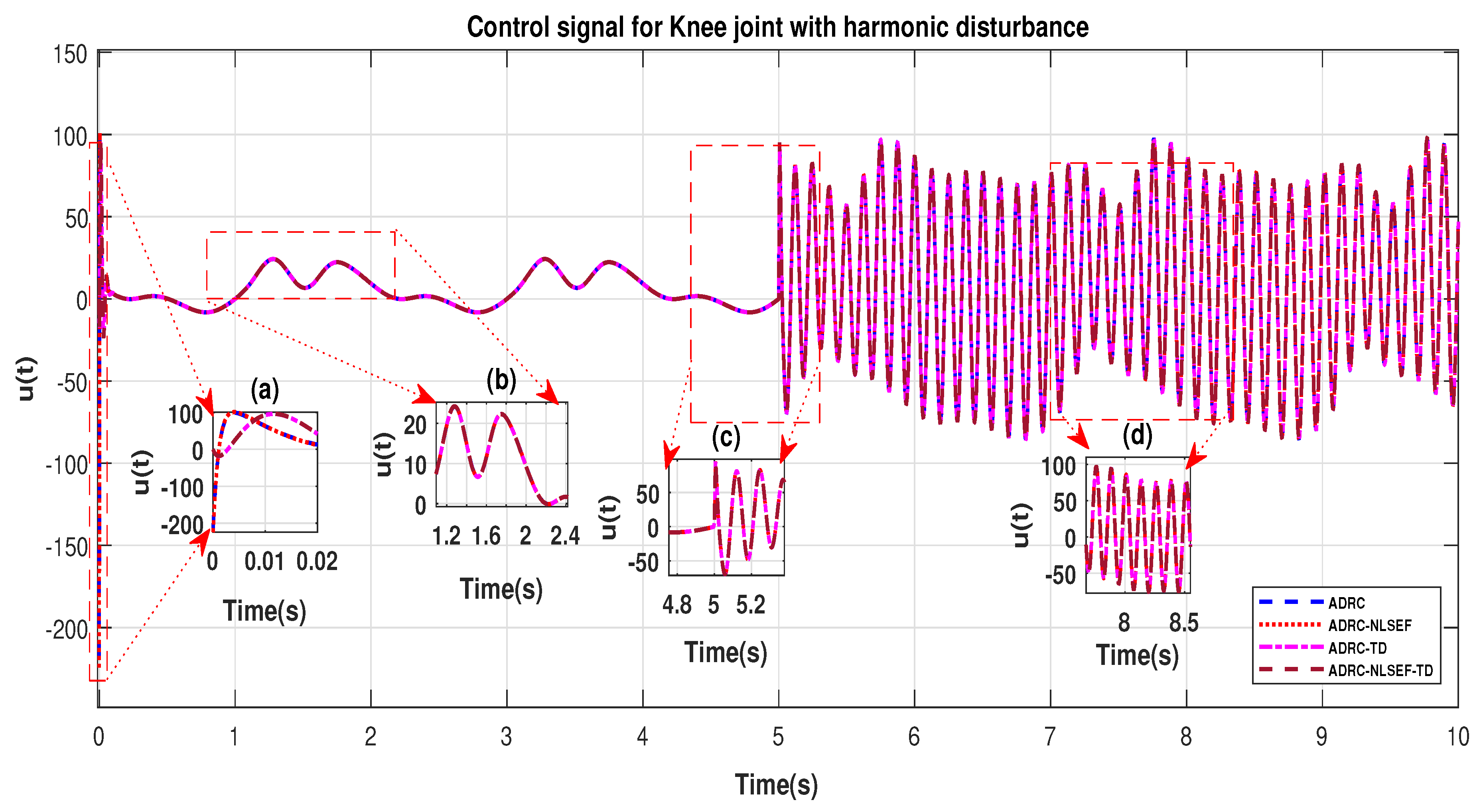
Figure 25.
Control signal comparison of ADRC, ADRC-NLSEF, ADRC-TD, and ADRC-NLSEF-TD for the knee joint with harmonic disturbance.
Figure 25.
Control signal comparison of ADRC, ADRC-NLSEF, ADRC-TD, and ADRC-NLSEF-TD for the knee joint with harmonic disturbance.
Figure 26.
Gait trajectory tracking error comparison of ADRC, ADRC-NLSEF, ADRC-TD, and ADRC-NLSEF-TD for the hip joint with a reference with harmonic disturbance.
Figure 26.
Gait trajectory tracking error comparison of ADRC, ADRC-NLSEF, ADRC-TD, and ADRC-NLSEF-TD for the hip joint with a reference with harmonic disturbance.
Figure 27.
Gait trajectory tracking error comparison of ADRC, ADRC-NLSEF, ADRC-TD, and ADRC-NLSEF-TD for the knee joint with a reference with harmonic disturbance.
Figure 27.
Gait trajectory tracking error comparison of ADRC, ADRC-NLSEF, ADRC-TD, and ADRC-NLSEF-TD for the knee joint with a reference with harmonic disturbance.
Figure 28.
Gait trajectory tracking comparison of ADRC, ADRC-NLSEF, ADRC-TD, and ADRC-NLSEF-TD for the hip joint under the influence of noise, with parameter variation and without disturbance effect.
Figure 28.
Gait trajectory tracking comparison of ADRC, ADRC-NLSEF, ADRC-TD, and ADRC-NLSEF-TD for the hip joint under the influence of noise, with parameter variation and without disturbance effect.
Figure 29.
Gait trajectory tracking comparison of ADRC, ADRC-NLSEF, ADRC-TD, and ADRC-NLSEF-TD for the knee joint under the influence of noise, with parameter variation and without disturbance effect.
Figure 29.
Gait trajectory tracking comparison of ADRC, ADRC-NLSEF, ADRC-TD, and ADRC-NLSEF-TD for the knee joint under the influence of noise, with parameter variation and without disturbance effect.
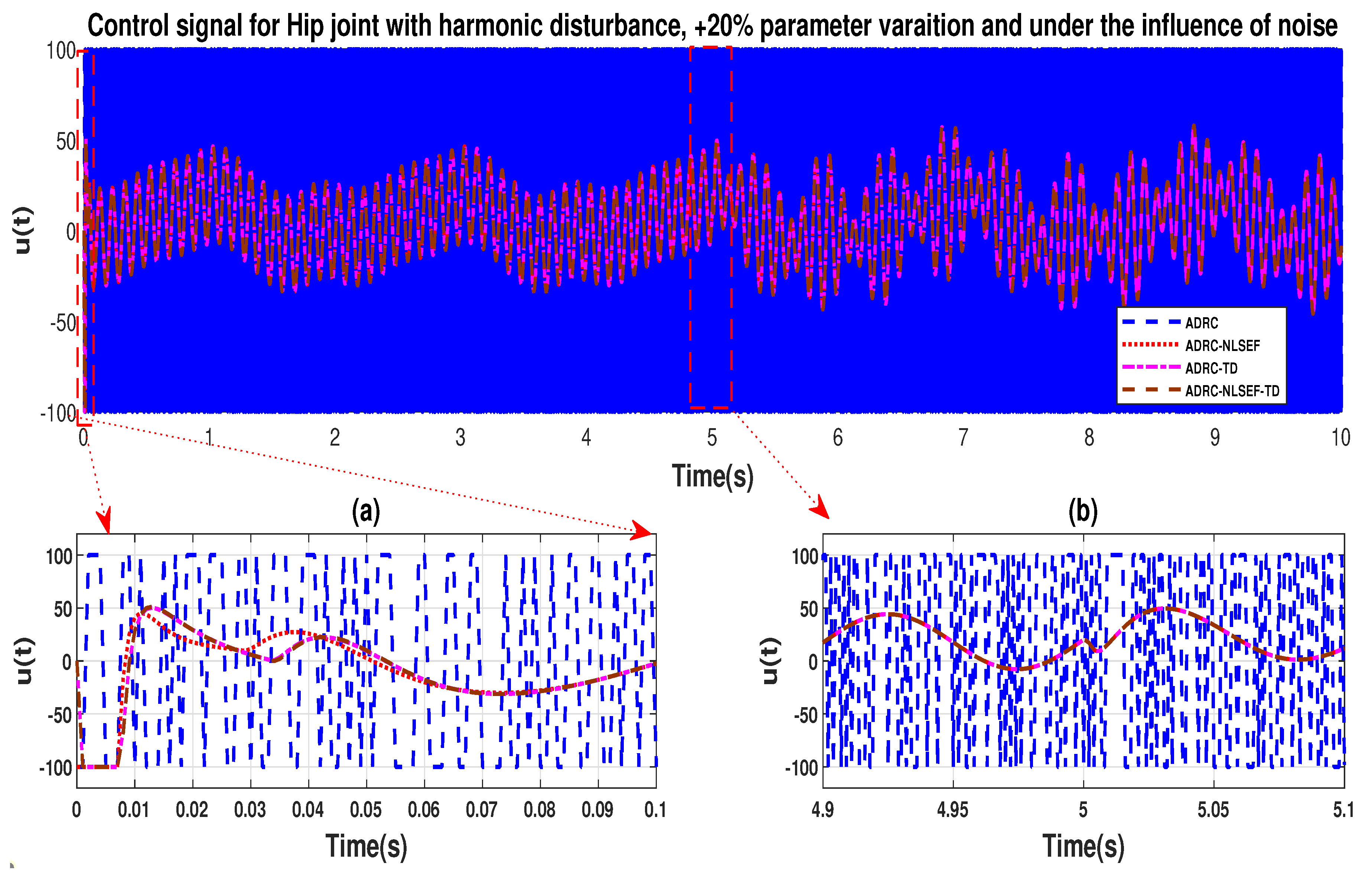
Figure 30.
Control signal trajectory tracking comparison of ADRC, ADRC-NLSEF, ADRC-TD, and ADRC-NLSEF-TD for the hip joint under the influence of noise, with parameter variation and without disturbance effect.
Figure 30.
Control signal trajectory tracking comparison of ADRC, ADRC-NLSEF, ADRC-TD, and ADRC-NLSEF-TD for the hip joint under the influence of noise, with parameter variation and without disturbance effect.
Figure 31.
Control signal trajectory tracking comparison of ADRC, ADRC-NLSEF, ADRC-TD, and ADRC-NLSEF-TD for the knee joint under the influence of noise, with parameter variation and without disturbance effect.
Figure 31.
Control signal trajectory tracking comparison of ADRC, ADRC-NLSEF, ADRC-TD, and ADRC-NLSEF-TD for the knee joint under the influence of noise, with parameter variation and without disturbance effect.
Figure 32.
Gait trajectory tracking error comparison of ADRC, ADRC-NLSEF, ADRC-TD, and ADRC-NLSEF-TD for the hip joint under the influence of noise, with parameter variation and without disturbance effect.
Figure 32.
Gait trajectory tracking error comparison of ADRC, ADRC-NLSEF, ADRC-TD, and ADRC-NLSEF-TD for the hip joint under the influence of noise, with parameter variation and without disturbance effect.
Figure 33.
Gait trajectory tracking error comparison of ADRC, ADRC-NLSEF, ADRC-TD, and ADRC-NLSEF-TD for the knee joint under the influence of noise, with parameter variation and without disturbance effect.
Figure 33.
Gait trajectory tracking error comparison of ADRC, ADRC-NLSEF, ADRC-TD, and ADRC-NLSEF-TD for the knee joint under the influence of noise, with parameter variation and without disturbance effect.
Figure 34.
Gait trajectory tracking comparison of ADRC, ADRC-NLSEF, ADRC-TD, and ADRC-NLSEF-TD for the hip joint under the influence of noise, with parameter variation and with random disturbance effect.
Figure 34.
Gait trajectory tracking comparison of ADRC, ADRC-NLSEF, ADRC-TD, and ADRC-NLSEF-TD for the hip joint under the influence of noise, with parameter variation and with random disturbance effect.
Figure 35.
Gait trajectory tracking comparison of ADRC, ADRC-NLSEF, ADRC-TD, and ADRC-NLSEF-TD for the knee joint under the influence of noise, with parameter variation and with random disturbance effect.
Figure 35.
Gait trajectory tracking comparison of ADRC, ADRC-NLSEF, ADRC-TD, and ADRC-NLSEF-TD for the knee joint under the influence of noise, with parameter variation and with random disturbance effect.
Figure 36.
Control signal trajectory tracking comparison of ADRC, ADRC-NLSEF, ADRC-TD, and ADRC-NLSEF-TD for the knee joint under the influence of noise, with parameter variation and with random disturbance effect.
Figure 36.
Control signal trajectory tracking comparison of ADRC, ADRC-NLSEF, ADRC-TD, and ADRC-NLSEF-TD for the knee joint under the influence of noise, with parameter variation and with random disturbance effect.
Figure 37.
Control signal trajectory tracking comparison of ADRC, ADRC-NLSEF, ADRC-TD, and ADRC-NLSEF-TD for the knee joint under the influence of noise, with parameter variation and with random disturbance effect.
Figure 37.
Control signal trajectory tracking comparison of ADRC, ADRC-NLSEF, ADRC-TD, and ADRC-NLSEF-TD for the knee joint under the influence of noise, with parameter variation and with random disturbance effect.
Figure 38.
Gait trajectory tracking error comparison of ADRC, ADRC-NLSEF, ADRC-TD, and ADRC-NLSEF-TD for the hip joint under the influence of noise, with parameter variation and with random disturbance effect.
Figure 38.
Gait trajectory tracking error comparison of ADRC, ADRC-NLSEF, ADRC-TD, and ADRC-NLSEF-TD for the hip joint under the influence of noise, with parameter variation and with random disturbance effect.
Figure 39.
Gait trajectory tracking error comparison of ADRC, ADRC-NLSEF, ADRC-TD, and ADRC-NLSEF-TD for the hip joint under the influence of noise, with parameter variation and with random disturbance effect.
Figure 39.
Gait trajectory tracking error comparison of ADRC, ADRC-NLSEF, ADRC-TD, and ADRC-NLSEF-TD for the hip joint under the influence of noise, with parameter variation and with random disturbance effect.
Figure 40.
Gait trajectory tracking comparison of ADRC, ADRC-NLSEF, ADRC-TD, and ADRC-NLSEF-TD for knee joint under the influence of noise, with parameter variation and with constant disturbance effect.
Figure 40.
Gait trajectory tracking comparison of ADRC, ADRC-NLSEF, ADRC-TD, and ADRC-NLSEF-TD for knee joint under the influence of noise, with parameter variation and with constant disturbance effect.
Figure 41.
Gait trajectory tracking comparison of ADRC, ADRC-NLSEF, ADRC-TD, and ADRC-NLSEF-TD for the knee joint under the influence of noise, with parameter variation and with constant disturbance effect.
Figure 41.
Gait trajectory tracking comparison of ADRC, ADRC-NLSEF, ADRC-TD, and ADRC-NLSEF-TD for the knee joint under the influence of noise, with parameter variation and with constant disturbance effect.
Figure 42.
Control signal trajectory tracking comparison of ADRC, ADRC-NLSEF, ADRC-TD, and ADRC-NLSEF-TD for the knee joint under the influence of noise, with parameter variation and with constant disturbance effect.
Figure 42.
Control signal trajectory tracking comparison of ADRC, ADRC-NLSEF, ADRC-TD, and ADRC-NLSEF-TD for the knee joint under the influence of noise, with parameter variation and with constant disturbance effect.
Figure 43.
Control signal trajectory tracking comparison of ADRC, ADRC-NLSEF, ADRC-TD, and ADRC-NLSEF-TD for the knee joint under the influence of noise, with parameter variation and with constant disturbance effect.
Figure 43.
Control signal trajectory tracking comparison of ADRC, ADRC-NLSEF, ADRC-TD, and ADRC-NLSEF-TD for the knee joint under the influence of noise, with parameter variation and with constant disturbance effect.
Figure 44.
Gait trajectory tracking error comparison of ADRC, ADRC-NLSEF, ADRC-TD, and ADRC-NLSEF-TD for hip joint under the influence of noise, with parameter variation and with constant disturbance effect.
Figure 44.
Gait trajectory tracking error comparison of ADRC, ADRC-NLSEF, ADRC-TD, and ADRC-NLSEF-TD for hip joint under the influence of noise, with parameter variation and with constant disturbance effect.
Figure 45.
Gait trajectory tracking error comparison of ADRC, ADRC-NLSEF, ADRC-TD, and ADRC-NLSEF-TD for hip joint under the influence of noise, with parameter variation and with constant disturbance effect.
Figure 45.
Gait trajectory tracking error comparison of ADRC, ADRC-NLSEF, ADRC-TD, and ADRC-NLSEF-TD for hip joint under the influence of noise, with parameter variation and with constant disturbance effect.
Figure 46.
Gait trajectory tracking comparison of ADRC, ADRC-NLSEF, ADRC-TD, and ADRC-NLSEF-TD for the knee joint under the influence of noise, with parameter variation and with harmonic disturbance effect.
Figure 46.
Gait trajectory tracking comparison of ADRC, ADRC-NLSEF, ADRC-TD, and ADRC-NLSEF-TD for the knee joint under the influence of noise, with parameter variation and with harmonic disturbance effect.
Figure 47.
Gait trajectory tracking comparison of ADRC, ADRC-NLSEF, ADRC-TD, and ADRC-NLSEF-TD for the knee joint under the influence of noise, with parameter variation and with harmonic disturbance effect.
Figure 47.
Gait trajectory tracking comparison of ADRC, ADRC-NLSEF, ADRC-TD, and ADRC-NLSEF-TD for the knee joint under the influence of noise, with parameter variation and with harmonic disturbance effect.
Figure 48.
Control signal trajectory tracking comparison of ADRC, ADRC-NLSEF, ADRC-TD, and ADRC-NLSEF-TD for the knee joint under the influence of noise, with parameter variation and with harmonic disturbance effect.
Figure 48.
Control signal trajectory tracking comparison of ADRC, ADRC-NLSEF, ADRC-TD, and ADRC-NLSEF-TD for the knee joint under the influence of noise, with parameter variation and with harmonic disturbance effect.
Figure 49.
Control signal trajectory tracking comparison of ADRC, ADRC-NLSEF, ADRC-TD, and ADRC-NLSEF-TD for the knee joint under the influence of noise, with parameter variation and with harmonic disturbance effect.
Figure 49.
Control signal trajectory tracking comparison of ADRC, ADRC-NLSEF, ADRC-TD, and ADRC-NLSEF-TD for the knee joint under the influence of noise, with parameter variation and with harmonic disturbance effect.
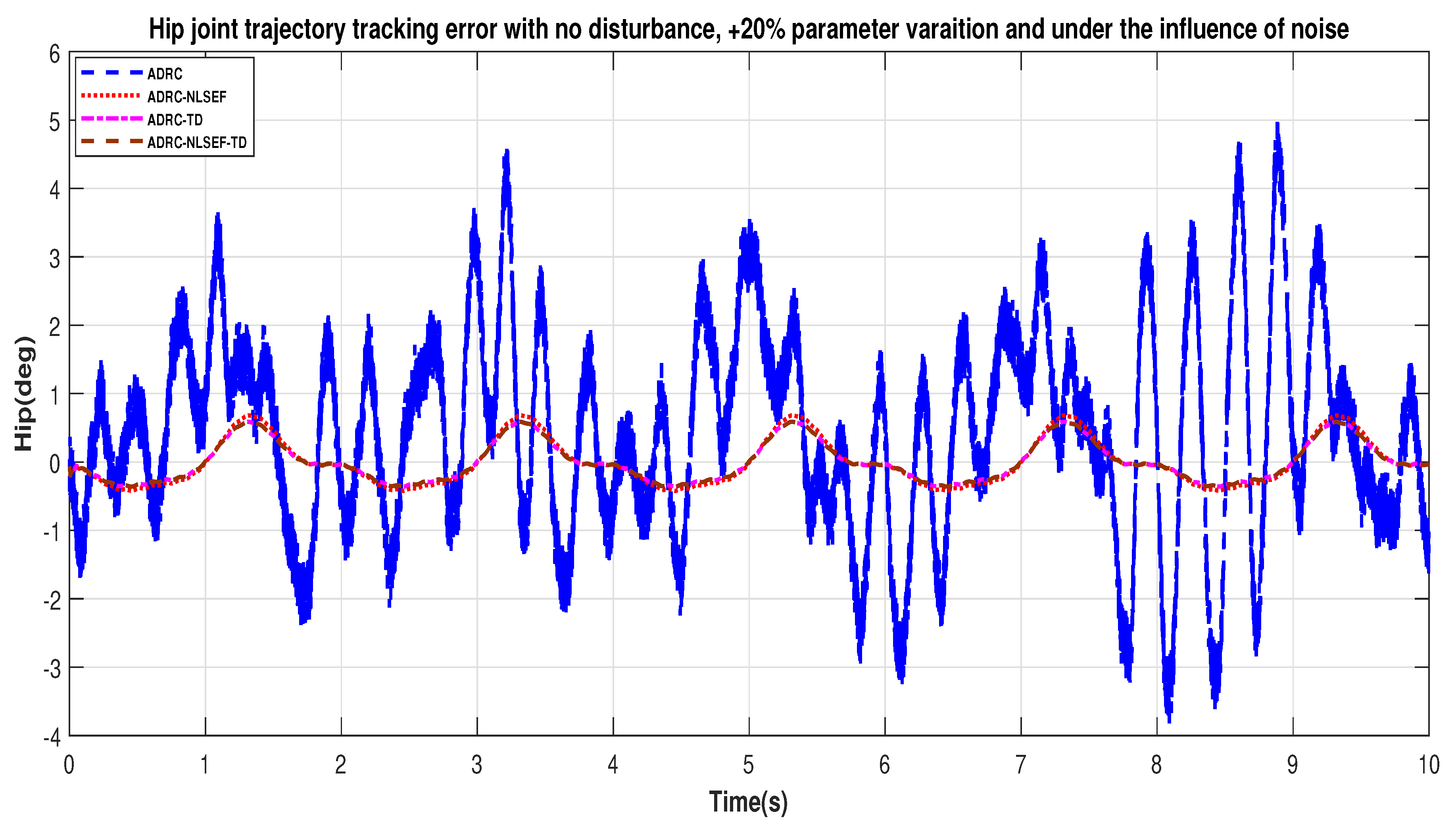
Figure 50.
Gait trajectory tracking error comparison of ADRC, ADRC-NLSEF, ADRC-TD, and ADRC-NLSEF-TD for the hip joint under the influence of noise, with parameter variation and with harmonic disturbance effect.
Figure 50.
Gait trajectory tracking error comparison of ADRC, ADRC-NLSEF, ADRC-TD, and ADRC-NLSEF-TD for the hip joint under the influence of noise, with parameter variation and with harmonic disturbance effect.
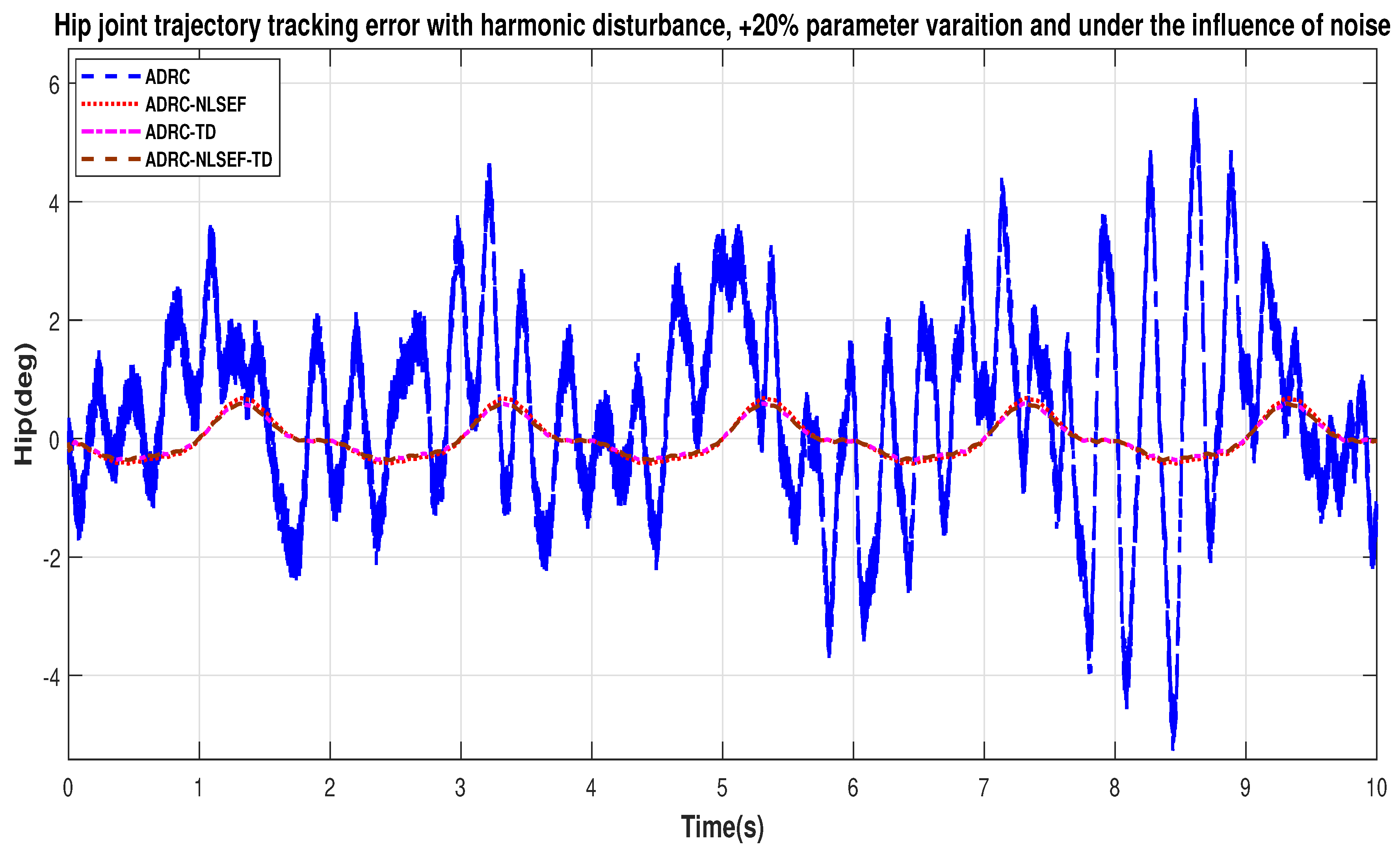
Figure 51.
Gait trajectory tracking error comparison of ADRC, ADRC-NLSEF, ADRC-TD, and ADRC-NLSEF-TD for the hip joint under the influence of noise, with parameter variation and with harmonic disturbance effect.
Figure 51.
Gait trajectory tracking error comparison of ADRC, ADRC-NLSEF, ADRC-TD, and ADRC-NLSEF-TD for the hip joint under the influence of noise, with parameter variation and with harmonic disturbance effect.
Table 1.
Parameters of the exoskeleton.
Table 1.
Parameters of the exoskeleton.
| Parameter | Symbol | Numerical Value |
|---|
| Thigh segment | | 5 kg |
| Length of thigh | | 435 mm |
| Length of shank | | 475 mm |
| Shank segment | | 2 kg |
| Gravity constant | g | 9.81 m/s |
Table 2.
Coefficients for the equation.
Table 2.
Coefficients for the equation.
| Coefficient | Value | Coefficient | Value |
|---|
| c | 0.208 | f | −0.103 |
| c | 0.362 | f | −0.010 |
| c | −0.066 | f | 0.029 |
| c | 0.001 | f | −0.342 |
| c | 0.766 | f | 0.168 |
| c | −0.099 | f | 0.084 |
| c | −0.219 | d | 3.142 |
| c | 0.008 | d | 3.142 |
Table 3.
The control law for proposed active disturbance rejection control (ADRC) with combinations
Table 3.
The control law for proposed active disturbance rejection control (ADRC) with combinations
| Controller | Control Law |
|---|
| ADRC | |
| ADRC-NLSEF | |
| ADRC-TD | |
| ADRC-NLSEF-TD | |
Table 4.
The parameters selection for tracking differentiator.
Table 4.
The parameters selection for tracking differentiator.
| Parameters | Variation | Final Selected Values |
|---|
| a | 5 to 50 | 30 |
| b and b | 1 to 10 | 5 |
| R | 10 to 80 | 30 |
| n | 1, 3, and 5 | 3 |
Table 5.
The parameters selection for NLSEF.
Table 5.
The parameters selection for NLSEF.
| Parameters | Variation | Final Selected Values |
|---|
| 0.5 to 1 | |
| 0.001 to 0.5 | |
Table 6.
Performance indices for ADRC, ADRC-NLSEF, ADRC-TD, and ADRC-NLSEF-TD for the hip joint and the knee joint for the no disturbance case.
Table 6.
Performance indices for ADRC, ADRC-NLSEF, ADRC-TD, and ADRC-NLSEF-TD for the hip joint and the knee joint for the no disturbance case.
| Control Method | | ADRC-NLSEF-TD | ADRC-TD | ADRC-NLSEF | ADRC |
|---|
| Joints | | Hip | Knee | Hip | Knee | Hip | Knee | Hip | Knee |
|---|
| Performance indices | ITSE (Deg.) | 4.241 | 13.2 | 4.253 | 13.32 | 5.793 | 17.95 | 6.083 | 18.87 |
| ISE (Deg.) | 0.8447 | 2.454 | 0.8468 | 2.477 | 1.152 | 3.332 | 1.209 | 3.503 |
| ITAE (Deg.) | 11.85 | 20.3 | 11.85 | 20.36 | 13.86 | 23.68 | 14.19 | 24.27 |
| IAE (Deg.) | 2.397 | 3.883 | 2.397 | 3.895 | 2.8 | 4.526 | 2.866 | 4.638 |
| ISU N.m.) | 0.1292 | 0.1739 | 0.1292 | 0.1738 | 0.1293 | 0.1724 | 0.1239 | 0.1722 |
Table 7.
Performance indices for ADRC, ADRC-NLSEF, ADRC-TD, and ADRC-NLSEF-TD for the hip joint and the knee joint for random disturbance case.
Table 7.
Performance indices for ADRC, ADRC-NLSEF, ADRC-TD, and ADRC-NLSEF-TD for the hip joint and the knee joint for random disturbance case.
| Control Method | | ADRC-NLSEF-TD | ADRC-TD | ADRC-NLSEF | ADRC |
|---|
| Joints | | Hip | Knee | Hip | Knee | Hip | Knee | Hip | Knee |
|---|
| Performance indices | ITSE (Deg.) | 4.241 | 13.2 | 4.253 | 13.32 | 5.793 | 17.95 | 6.082 | 18.87 |
| ISE (Deg.) | 0.8447 | 2.454 | 0.8468 | 2.477 | 1.152 | 3.332 | 1.209 | 3.503 |
| ITAE (Deg.) | 11.85 | 20.3 | 11.85 | 20.36 | 13.86 | 23.68 | 14.19 | 24.27 |
| IAE (Deg.) | 2.397 | 3.883 | 2.397 | 3.895 | 2.8 | 4.526 | 2.866 | 4.638 |
| ISU (N.m.) | 0.1298 | 0.1817 | 0.1298 | 0.1817 | 0.1299 | 0.1803 | 0.1299 | 0.1801 |
Table 8.
Performance indices for ADRC, ADRC-NLSEF, ADRC-TD, and ADRC-NLSEF-TD for the hip joint and the knee joint for the constant disturbance case.
Table 8.
Performance indices for ADRC, ADRC-NLSEF, ADRC-TD, and ADRC-NLSEF-TD for the hip joint and the knee joint for the constant disturbance case.
| Control Method | | ADRC-NLSEF-TD | ADRC-TD | ADRC-NLSEF | ADRC |
|---|
| Joints | | Hip | Knee | Hip | Knee | Hip | Knee | Hip | Knee |
|---|
| Performance indices | ITSE (Deg.) | 4.241 | 13.21 | 4.252 | 13.34 | 5.792 | 17.96 | 6.081 | 18.89 |
| ISE (Deg.) | 0.8446 | 2.456 | 0.8466 | 2.478 | 1.152 | 3.334 | 1.209 | 3.505 |
| ITAE (Deg.) | 11.85 | 20.31 | 11.85 | 20.37 | 13.86 | 23.69 | 14.19 | 24.28 |
| IAE (Deg.) | 2.397 | 3.884 | 2.398 | 3.896 | 2.8 | 4.527 | 2.866 | 4.639 |
| ISU (N.m.) | 0.6217 | 3.167 | 0.6217 | 3.167 | 0.6214 | 3.166 | 0.6214 | 3.166 |
Table 9.
Performance indices for ADRC, ADRC-NLSEF, ADRC-TD, and ADRC-NLSEF-TD for the hip joint and the knee joint for harmonic disturbance case.
Table 9.
Performance indices for ADRC, ADRC-NLSEF, ADRC-TD, and ADRC-NLSEF-TD for the hip joint and the knee joint for harmonic disturbance case.
| Control Method | | ADRC-NLSEF-TD | ADRC-TD | ADRC-NLSEF | ADRC |
|---|
| Joints | | Hip | Knee | Hip | Knee | Hip | Knee | Hip | Knee |
|---|
| Performance indices | ITSE (Deg.) | 4.243 | 13.22 | 4.255 | 13.34 | 5.795 | 17.97 | 6.085 | 18.89 |
| ISE (Deg.) | 0.845 | 2.457 | 0.847 | 2.48 | 1.152 | 3.335 | 1.21 | 3.506 |
| ITAE (Deg.) | 11.86 | 20.35 | 11.86 | 20.41 | 13.87 | 23.73 | 14.2 | 24.32 |
| IAE (Deg.) | 2.399 | 3.89 | 2.399 | 3.902 | 2.801 | 4.533 | 2.867 | 4.645 |
| ISU (N.m.) | 0.3034 | 2.039 | 0.3035 | 2.041 | 0.3035 | 2.038 | 0.3037 | 2.039 |
Table 10.
Overall performance indices the hip joint.
Table 10.
Overall performance indices the hip joint.
| Hip Joint |
|---|
| Control Method | Disturbance Case | ITSE (Deg.) | ISE (Deg.) | ITAE (Deg.) | IAE (Deg.) | ISU (N.m.)
|
|---|
| ADRC-NLSEF-TD | Case 1 | 4.241 | 0.8447 | 11.85 | 2.397 | 0.1292 |
| Case 2 | 4.241 | 0.8447 | 11.85 | 2.397 | 0.1298 |
| Case 3 | 4.241 | 0.8446 | 11.85 | 2.397 | 0.6217 |
| Case 4 | 4.243 | 0.8450 | 11.86 | 2.399 | 0.3034 |
| ADRC-TD | Case 1 | 4.253 | 0.8468 | 11.85 | 2.397 | 0.1292 |
| Case 2 | 4.253 | 0.8468 | 11.85 | 2.397 | 0.1298 |
| Case 3 | 4.252 | 0.8466 | 11.85 | 2.398 | 0.6217 |
| Case 4 | 4.255 | 0.8470 | 11.86 | 2.399 | 0.3035 |
| ADRC-NLSEF | Case 1 | 5.793 | 1.152 | 13.86 | 2.800 | 0.1293 |
| Case 2 | 5.793 | 1.152 | 13.86 | 2.800 | 0.1299 |
| Case 3 | 5.792 | 1.152 | 13.86 | 2.800 | 0.6214 |
| Case 4 | 5.795 | 1.152 | 13.87 | 2.801 | 0.3035 |
| ADRC | Case 1 | 6.083 | 1.209 | 14.19 | 2.866 | 0.1293 |
| Case 2 | 6.082 | 1.209 | 14.19 | 2.866 | 0.1299 |
| Case 3 | 6.081 | 1.209 | 14.19 | 2.866 | 0.6214 |
| Case 4 | 6.085 | 1.21 | 14.20 | 2.867 | 0.3037 |
Table 11.
Overall performance indices for the knee joint.
Table 11.
Overall performance indices for the knee joint.
| Knee Joint |
|---|
| Control Method | Disturbance Case | ITSE (Deg.) | ISE (Deg.) | ITAE (Deg.) | IAE (Deg.) | ISU (N.m.)
|
|---|
| ADRC-NLSEF-TD | Case 1 | 13.20 | 2.454 | 20.30 | 3.883 | 0.1739 |
| Case 2 | 13.20 | 2.454 | 20.30 | 3.883 | 0.1818 |
| Case 3 | 13.21 | 2.456 | 20.31 | 3.884 | 3.167 |
| Case 4 | 13.22 | 2.457 | 20.35 | 3.890 | 2.039 |
| ADRC-TD | Case 1 | 13.32 | 2.477 | 20.36 | 3.895 | 0.1738 |
| Case 2 | 13.32 | 2.477 | 20.36 | 3.895 | 0.1817 |
| Case 3 | 13.34 | 2.478 | 20.37 | 3.896 | 3.167 |
| Case 4 | 13.34 | 2.48 | 20.41 | 3.902 | 2.041 |
| ADRC-NLSEF | Case 1 | 17.95 | 3.332 | 23.68 | 4.526 | 0.1724 |
| Case 2 | 17.95 | 3.332 | 23.68 | 4.526 | 0.1803 |
| Case 3 | 17.96 | 3.334 | 22.69 | 4.527 | 3.166 |
| Case 4 | 17.97 | 3.335 | 22.73 | 4.533 | 2.038 |
| ADRC | Case 1 | 18.87 | 3.503 | 24.27 | 4.638 | 0.1722 |
| Case 2 | 18.87 | 3.503 | 24.27 | 4.638 | 0.1801 |
| Case 3 | 18.89 | 3.505 | 24.28 | 4.639 | 3.166 |
| Case 4 | 18.89 | 3.506 | 27.32 | 4.645 | 2.039 |
Table 12.
Parameters of the exoskeleton.
Table 12.
Parameters of the exoskeleton.
| Parameter | Symbol | Numerical Value (Actual) | −20% Varied Values | 20% Varied Values |
|---|
| Thigh segment | | 5 kg | 4 Kg | 6 kg |
| length of thigh | | 435 mm | 348 mm | 522 mm |
| Length of shank | | 475 mm | 380 mm | 570 mm |
| Shank segment | | 2 kg | 1.6 kg | 2.4 kg |
Table 13.
Overall performance indices of the hip joint parameter variation.
Table 13.
Overall performance indices of the hip joint parameter variation.
| Hip Joint |
|---|
| | | ITSE (Deg.) | ISE (Deg.) | ITAE (Deg.) | IAE (Deg.) | ISU (N.m.)
|
|---|
| Control Method | Disturbance Case | −20% | +20% | −20% | +20% | −20% | +20% | −20% | +20 | −20% | +20% |
|---|
| ADRC-TD-NLSEF | Case 1 | 4.240 | 4.242 | 0.8444 | 0.8448 | 11.85 | 11.85 | 2.397 | 2.397 | 0.1829 | 0.09875 |
| Case 2 | 4.240 | 4.242 | 0.8444 | 0.8448 | 11.85 | 11.85 | 2.397 | 2.397 | 0.1850 | 0.09897 |
| Case 3 | 4.238 | 4.241 | 0.8441 | 0.8447 | 11.85 | 11.85 | 2.397 | 2.398 | 1.848 | 0.2869 |
| Case 4 | 4.252 | 4.243 | 0.846 | 0.8449 | 11.88 | 11.86 | 2.401 | 2.398 | 0.8465 | 0.1572 |
| ADRC-TD | Case 1 | 4.251 | 4.253 | 0.8464 | 0.8468 | 11.85 | 11.85 | 2.397 | 2.398 | 0.1829 | 0.09875 |
| Case 2 | 4.251 | 4.253 | 0.8464 | 0.8468 | 11.85 | 11.85 | 2.397 | 2.398 | 0.1850 | 0.09897 |
| Case 3 | 4.249 | 4.252 | 0.8461 | 0.8467 | 11.85 | 11.85 | 2.397 | 2.398 | 1.848 | 0.2869 |
| Case 4 | 4.264 | 4.254 | 0.8481 | 0.847 | 11.88 | 11.86 | 2.401 | 2.398 | 0.8470 | 0.1572 |
| ADRC-NLSEF | Case 1 | 5.791 | 5.793 | 1.152 | 1.152 | 13.85 | 13.86 | 2.799 | 2.8 | 0.1830 | 0.09894 |
| Case 2 | 5.791 | 5.793 | 1.152 | 1.152 | 13.85 | 13.86 | 2.799 | 2.8 | 0.1851 | 0.09916 |
| Case 3 | 5.789 | 5.793 | 1.151 | 1.152 | 13.86 | 13.86 | 2.799 | 2.8 | 1.848 | 0.2871 |
| Case 4 | 5.803 | 5.794 | 1.153 | 1.152 | 13.88 | 13.86 | 2.803 | 2.8 | 0.8467 | 0.1574 |
| ADRC | Case 1 | 6.081 | 6.083 | 1.209 | 1.21 | 14.19 | 14.19 | 2.866 | 2.866 | 0.1830 | 0.09892 |
| Case 2 | 6.081 | 6.083 | 1.209 | 1.21 | 14.19 | 14.19 | 2.866 | 2.866 | 0.1851 | 0.09914 |
| Case 3 | 6.078 | 6.082 | 1.209 | 1.209 | 14.19 | 14.19 | 2.866 | 2.866 | 1.848 | 0.2871 |
| Case 4 | 6.093 | 6.084 | 1.211 | 1.21 | 14.22 | 14.19 | 2.87 | 2.867 | 0.8472 | 0.1574 |
Table 14.
Overall performance indices of the knee joint parameter variation.
Table 14.
Overall performance indices of the knee joint parameter variation.
| Knee Joint |
|---|
| | | ITSE (Deg.) | ISE (Deg.) | ITAE (Deg.) | IAE (Deg.) | ISU (N.m.)
|
|---|
| Control Method | Disturbance Case | −20% | +20% | −20% | +20% | −20% | +20% | −20% | +20 | −20% | +20% |
|---|
| ADRC-TD-NLSEF | Case 1 | 13.20 | 13.2 | 2.456 | 2.454 | 20.3 | 20.3 | 3.885 | 3.883 | 0.2489 | 0.1362 |
| Case 2 | 13.21 | 13.2 | 2.456 | 2.454 | 20.3 | 20.3 | 3.885 | 3.883 | 0.2759 | 0.1392 |
| Case 3 | 13.24 | 13.21 | 2.459 | 2.455 | 20.32 | 20.3 | 3.886 | 3.884 | 12.76 | 1.009 |
| Case 4 | 13.31 | 13.21 | 2.47 | 2.455 | 20.44 | 20.33 | 3.903 | 3.888 | 7.372 | 0.7600 |
| ADRC-TD | Case 1 | 13.33 | 13.32 | 2.478 | 2.477 | 20.37 | 20.36 | 3.896 | 3.895 | 0.2489 | 0.1361 |
| Case 2 | 13.33 | 13.32 | 2.478 | 2.477 | 20.37 | 20.36 | 3.896 | 3.895 | 0.2757 | 0.1391 |
| Case 3 | 13.36 | 13.33 | 2.482 | 2.478 | 20.39 | 20.37 | 3.898 | 3.895 | 12.76 | 1.009 |
| Case 4 | 13.44 | 13.33 | 2.493 | 2.478 | 20.51 | 20.4 | 3.916 | 3.899 | 7.377 | 0.7604 |
| ADRC-NLSEF | Case 1 | 17.96 | 17.95 | 3.333 | 3.332 | 23.69 | 23.68 | 4.527 | 4.526 | 0.2475 | 0.1347 |
| Case 2 | 17.96 | 17.95 | 3.333 | 3.332 | 23.69 | 23.68 | 4.527 | 4.526 | 0.2744 | 0.1377 |
| Case 3 | 17.99 | 17.96 | 3.338 | 3.333 | 23.71 | 23.69 | 4.529 | 4.526 | 12.76 | 1.008 |
| Case 4 | 18.07 | 17.96 | 3.348 | 3.333 | 23.83 | 23.72 | 4.546 | 4.531 | 7.372 | 0.7586 |
| ADRC | Case 1 | 18.88 | 18.87 | 3.504 | 3.503 | 24.28 | 24.27 | 4.639 | 4.638 | 0.2473 | 0.1345 |
| Case 2 | 18.88 | 18.87 | 3.504 | 3.503 | 24.27 | 24.27 | 4.639 | 4.638 | 0.2741 | 0.1375 |
| Case 3 | 18.92 | 18.88 | 3.509 | 3.504 | 24.29 | 24.27 | 4.461 | 4.638 | 12.76 | 1.007 |
| Case 4 | 18.99 | 18.88 | 3.52 | 3.504 | 24.42 | 24.31 | 4.658 | 4.642 | 7.376 | 0.7588 |
Table 15.
Overall performance indices of the hip joint parameter variation and under influence of noise.
Table 15.
Overall performance indices of the hip joint parameter variation and under influence of noise.
| Hip Joint |
|---|
| Control Method | Disturbance Case | ITSE (Deg.) | ISE (Deg.) | ITAE (Deg.) | IAE (Deg.) | ISU (N.m.)
|
|---|
| ADRC-TD-NLSEF | Case 1 | 4.244 | 0.8461 | 11.87 | 2.404 | 0.7248 |
| Case 2 | 4.244 | 0.8461 | 11.87 | 2.404 | 0.7277 |
| Case 3 | 4.243 | 0.8460 | 11.87 | 2.404 | 0.9132 |
| Case 4 | 4.245 | 0.8462 | 11.87 | 2.404 | 0.7802 |
| ADRC-TD | Case 1 | 4.256 | 0.8482 | 11.87 | 2.404 | 0.7252 |
| Case 2 | 4.256 | 0.8482 | 11.87 | 2.404 | 0.7281 |
| Case 3 | 4.255 | 0.8481 | 11.87 | 2.404 | 0.9135 |
| Case 4 | 4.257 | 0.8483 | 11.87 | 2.405 | 0.7806 |
| ADRC-NLSEF | Case 1 | 5.796 | 1.153 | 13.87 | 2.805 | 0.7239 |
| Case 2 | 5.796 | 1.153 | 13.87 | 2.805 | 0.7269 |
| Case 3 | 5..795 | 1.153 | 13.87 | 2.805 | 0.9123 |
| Case 4 | 5.797 | 1.153 | 13.88 | 2.805 | 0.7794 |
| ADRC | Case 1 | 144 | 25.03 | 67.94 | 12.69 | 9.914 |
| Case 2 | 150.7 | 25.79 | 68.39 | 12.73 | 9.906 |
| Case 3 | 380.5 | 56.62 | 110.5 | 18.38 | 9.914 |
| Case 4 | 173.9 | 29.17 | 73.35 | 13.48 | 9.912 |
Table 16.
Overall performance indices of the Knee joint parameter variation and under influence of noise.
Table 16.
Overall performance indices of the Knee joint parameter variation and under influence of noise.
| Knee Joint |
|---|
| Control Method | Disturbance Case | ITSE (Deg.) | ISE (Deg.) | ITAE (Deg.) | IAE (Deg.) | ISU (N.m.)
|
|---|
| ADRC-TD-NLSEF | Case 1 | 13.20 | 2.464 | 20.31 | 3.894 | 0.8040 |
| Case 2 | 13.20 | 2.464 | 20.31 | 3.894 | 0.8240 |
| Case 3 | 13.21 | 2.465 | 20.32 | 3.894 | 1.659 |
| Case 4 | 13.21 | 2.465 | 20.34 | 3.898 | 1.44 |
| ADRC-TD | Case 1 | 13.32 | 2.486 | 20.38 | 3.905 | 0.8031 |
| Case 2 | 13.33 | 2.486 | 20.38 | 3.905 | 0.8230 |
| Case 3 | 13.33 | 2.487 | 20.38 | 3.906 | 1.658 |
| Case 4 | 13.34 | 2.488 | 20.41 | 3.910 | 1.439 |
| ADRC-NLSEF | Case 1 | 17.95 | 3.338 | 23.70 | 4.535 | 0.7989 |
| Case 2 | 17.95 | 3.338 | 23.70 | 4.535 | 0.8189 |
| Case 3 | 17.96 | 3.339 | 23.71 | 4.536 | 1.655 |
| Case 4 | 17.96 | 3.340 | 23.73 | 4.540 | 1.434 |
| ADRC | Case 1 | 734.7 | 121.7 | 146.4 | 27.1 | 9.716 |
| Case 2 | 776.1 | 126.3 | 149.3 | 27.4 | 9.730 |
| Case 3 | 2149 | 308.7 | 253 | 41.37 | 9.742 |
| Case 4 | 873.6 | 140.7 | 157.2 | 28.78 | 9.742 |

 ,
, 


