A Low-Cost, High-Precision Vehicle Navigation System for Deep Urban Multipath Environment Using TDCP Measurements †

 ,
,
Abstract
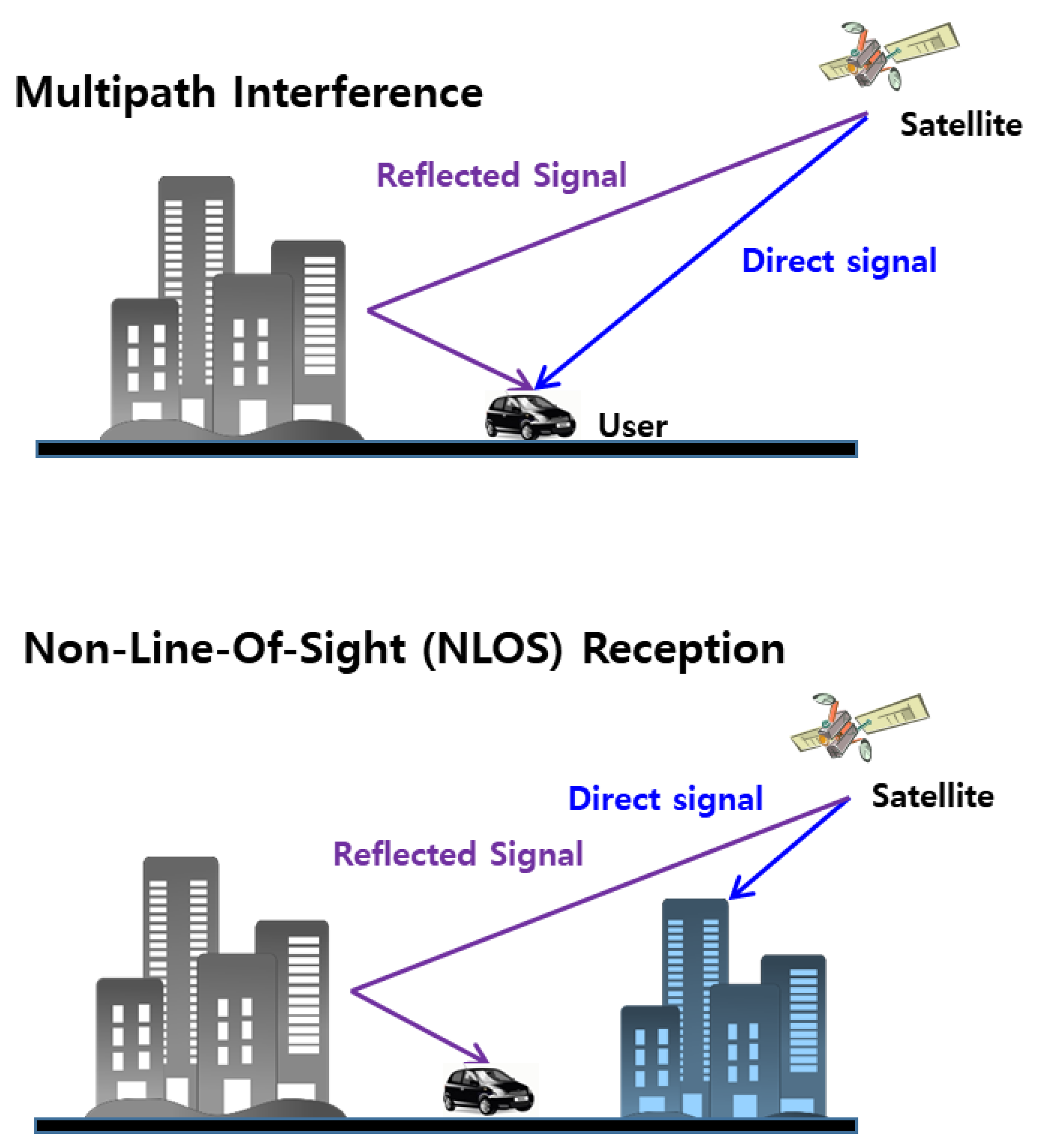
:1. Introduction
2. System Overview
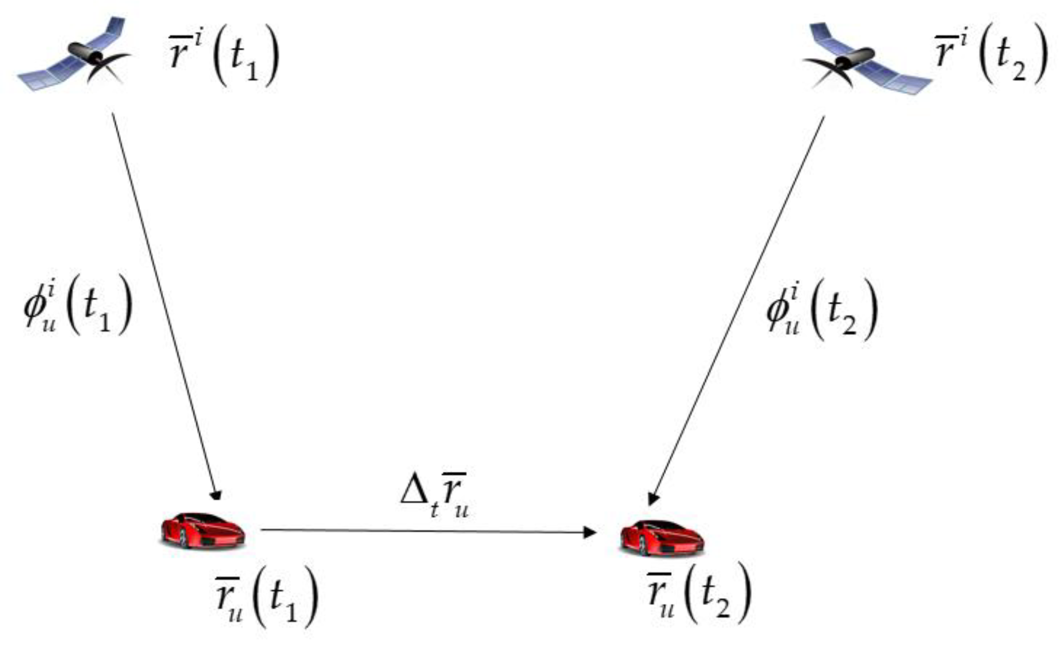
2.1. Time-Differenced Carrier Phase (TDCP) Measurements
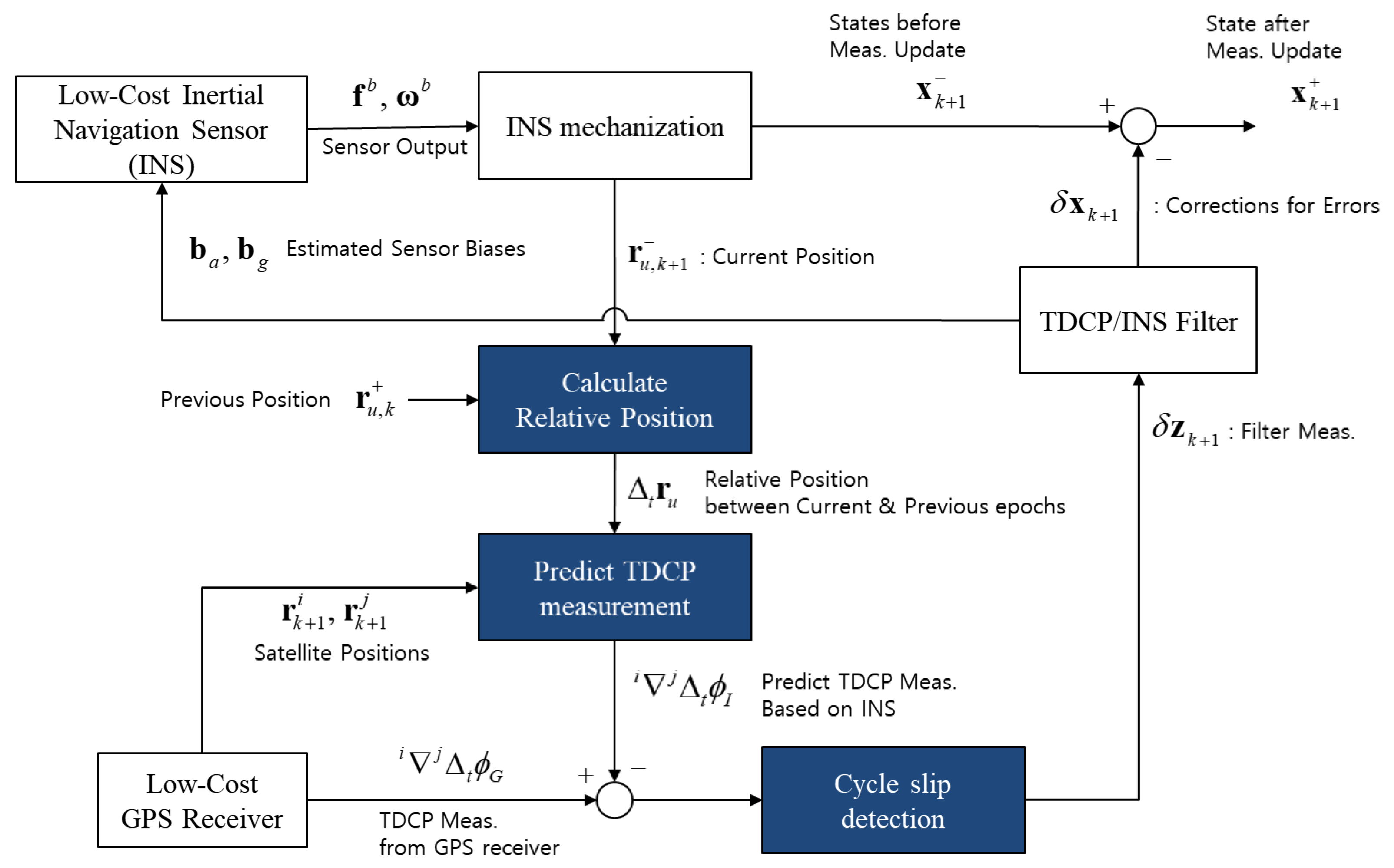
2.2. TDCP/INS Integrated Navigation System
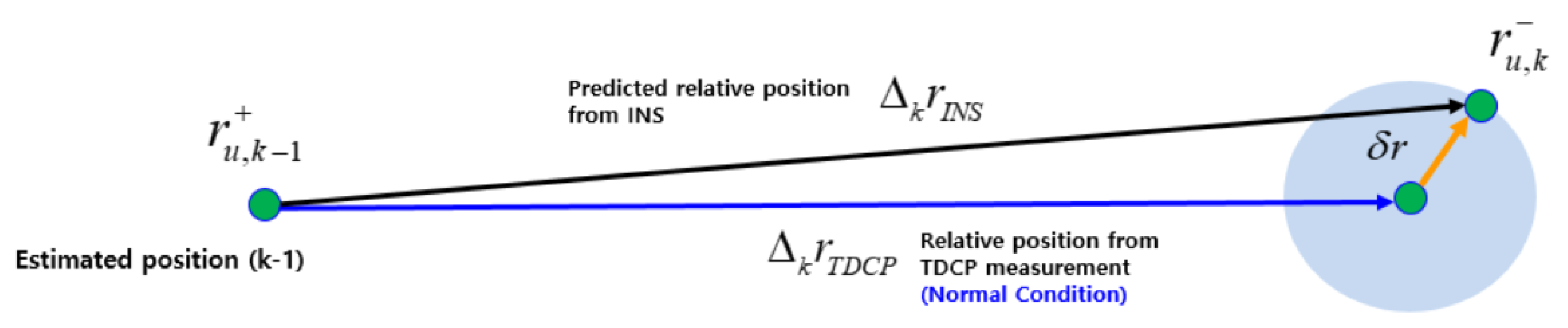
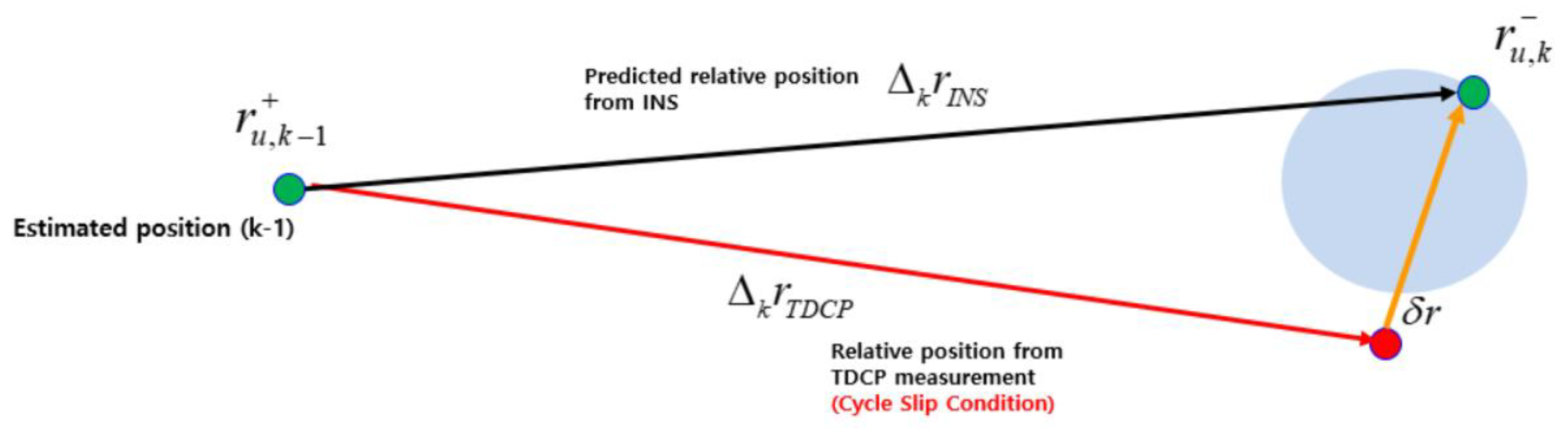
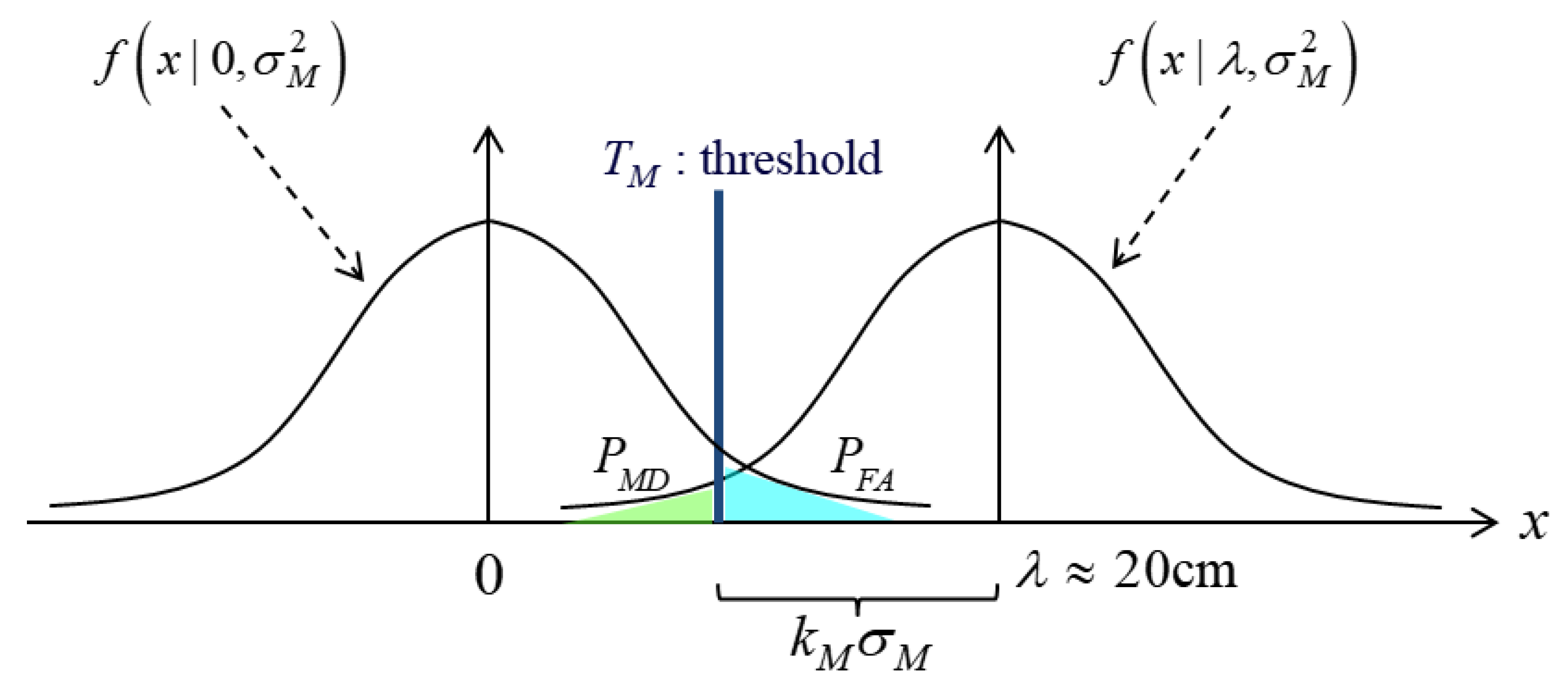
2.3. Cycle Slip Detection Algorithm
3. Dynamic Test in Deep Urban Multipath Environment
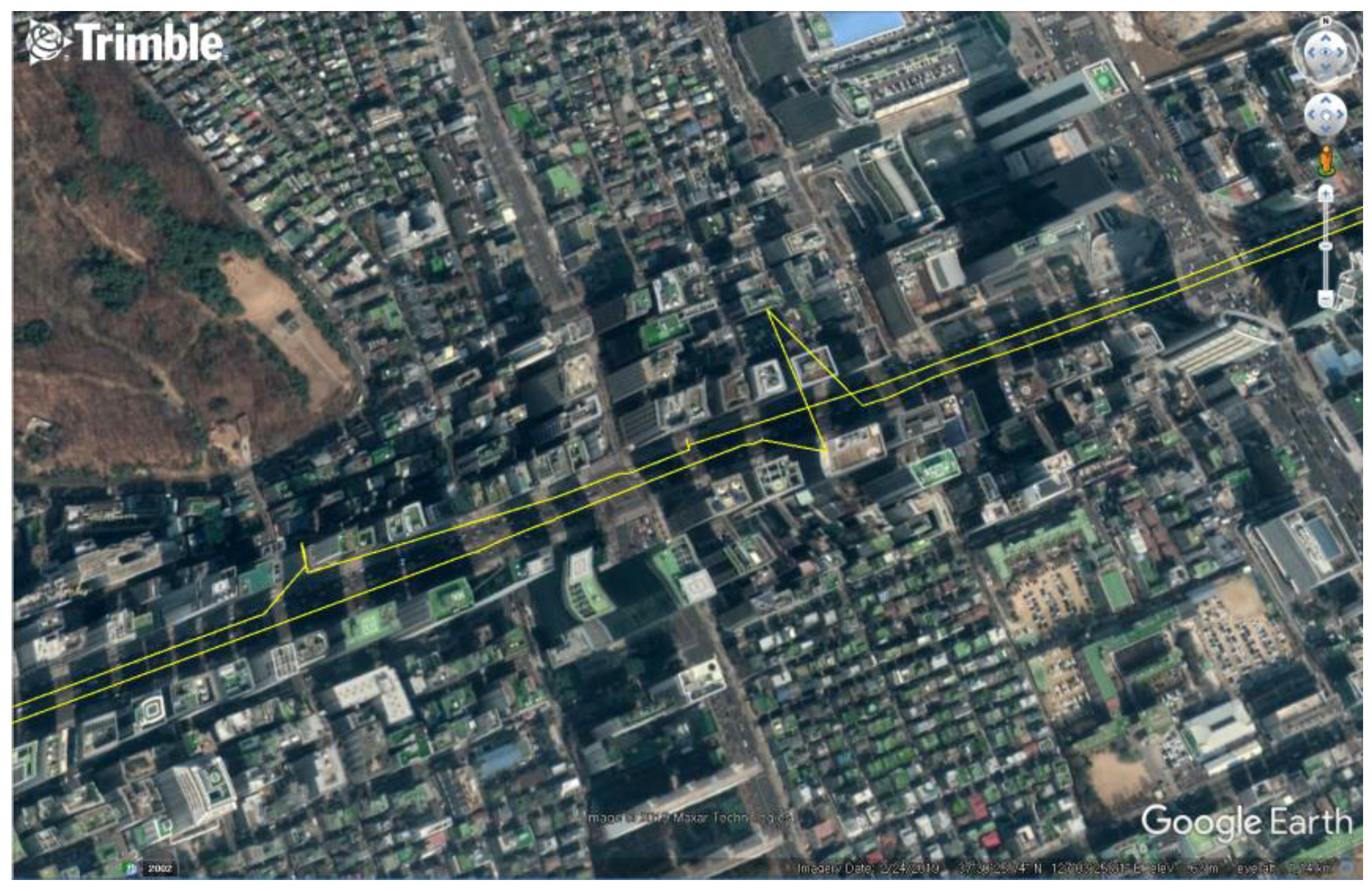
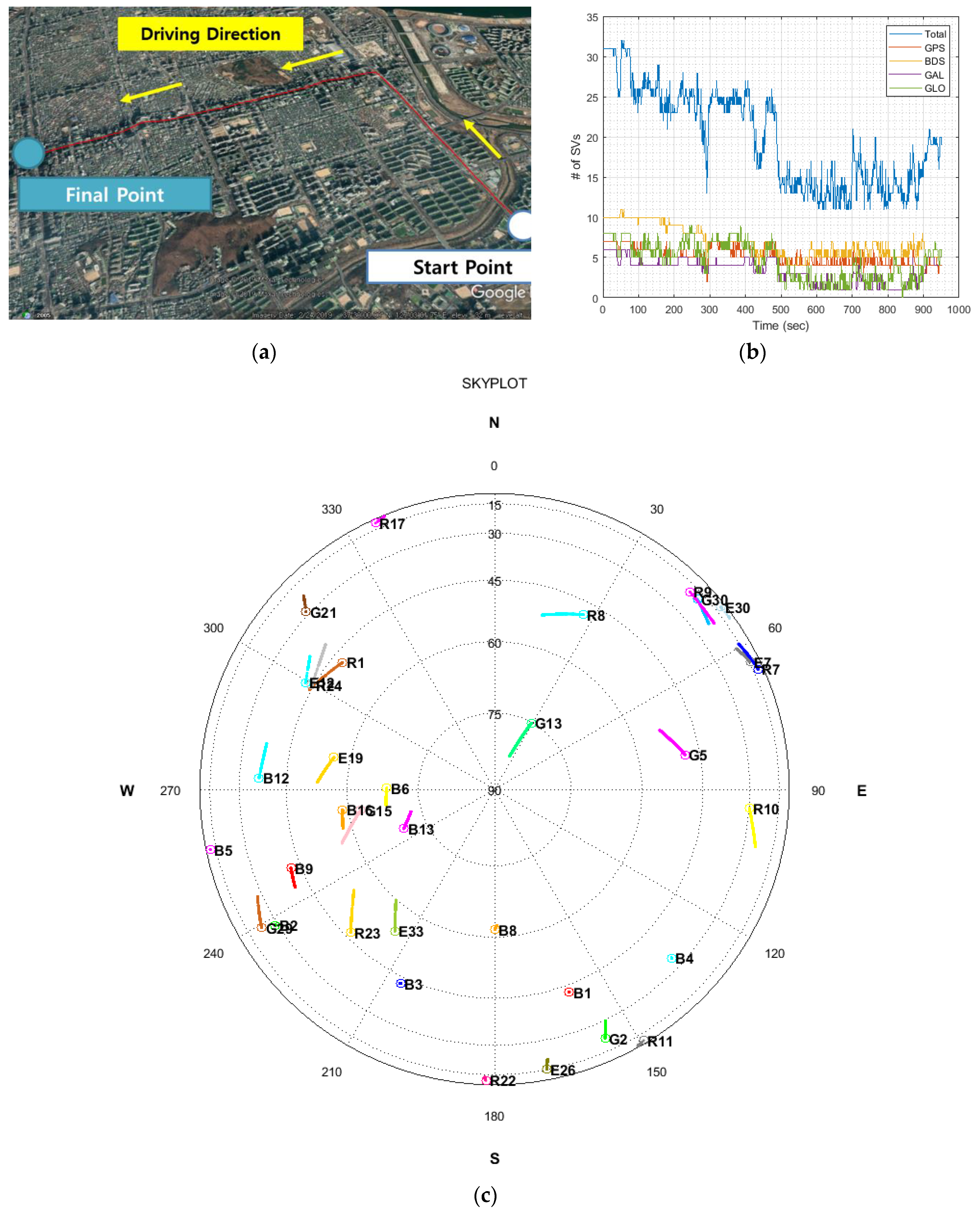
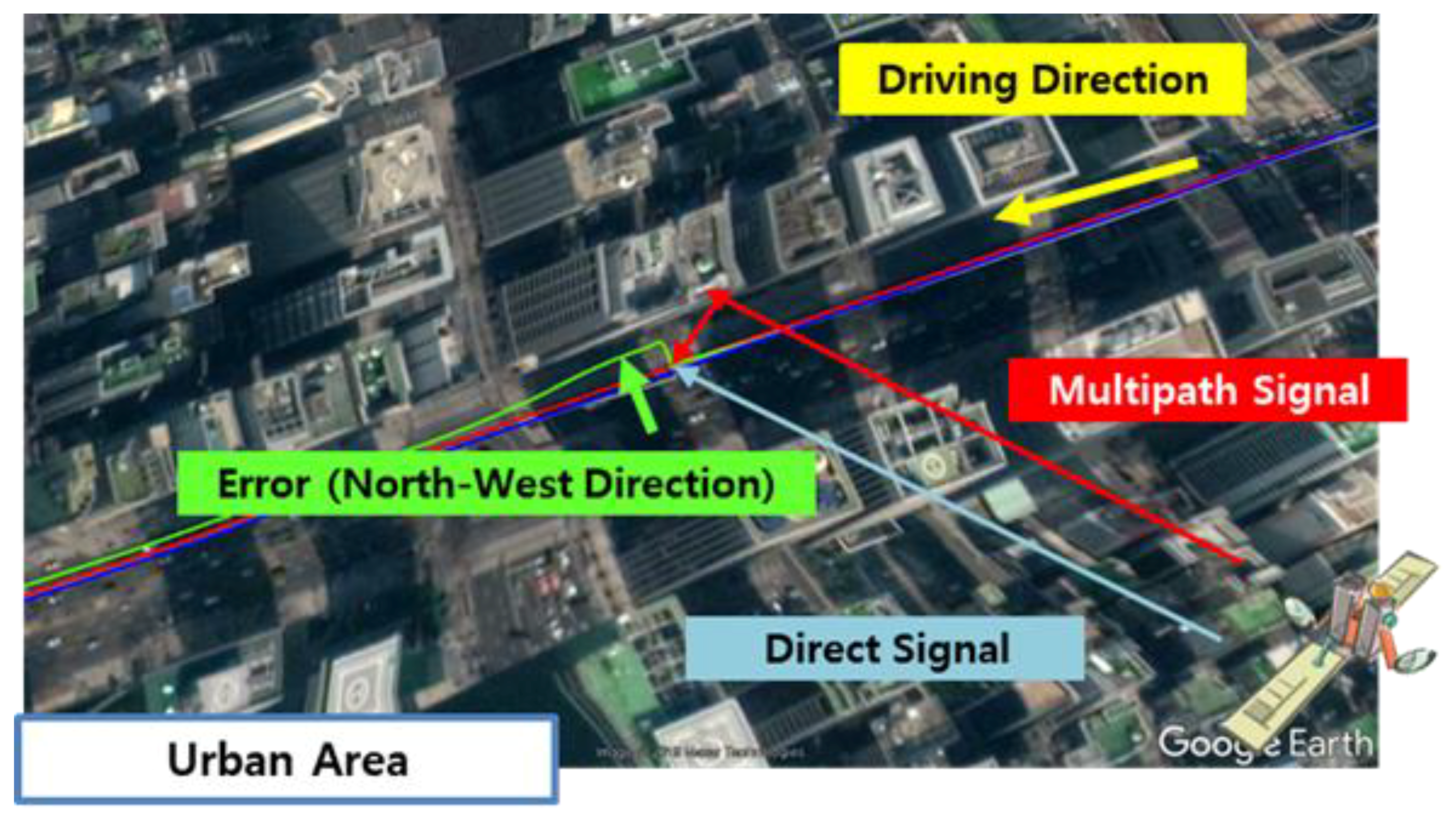
3.1. Test Environment
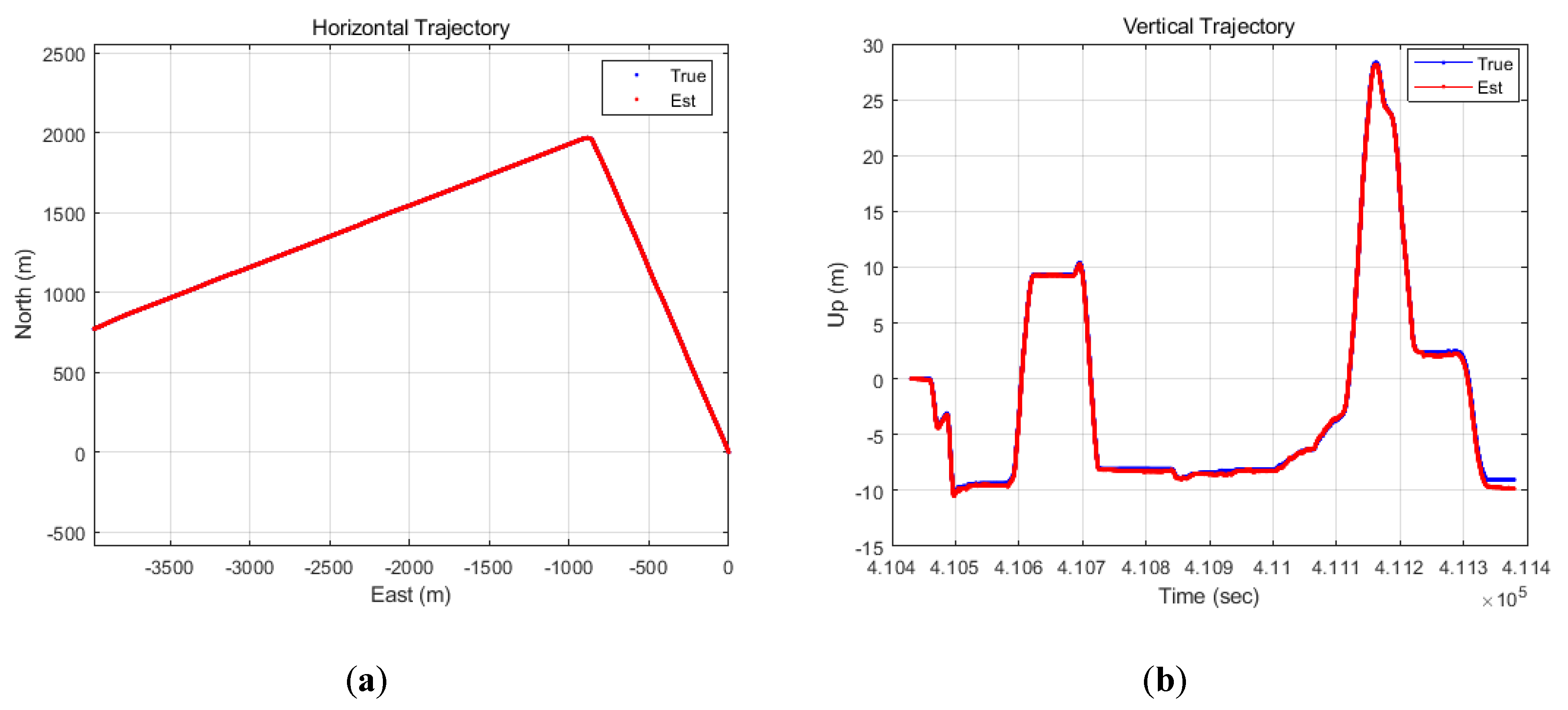
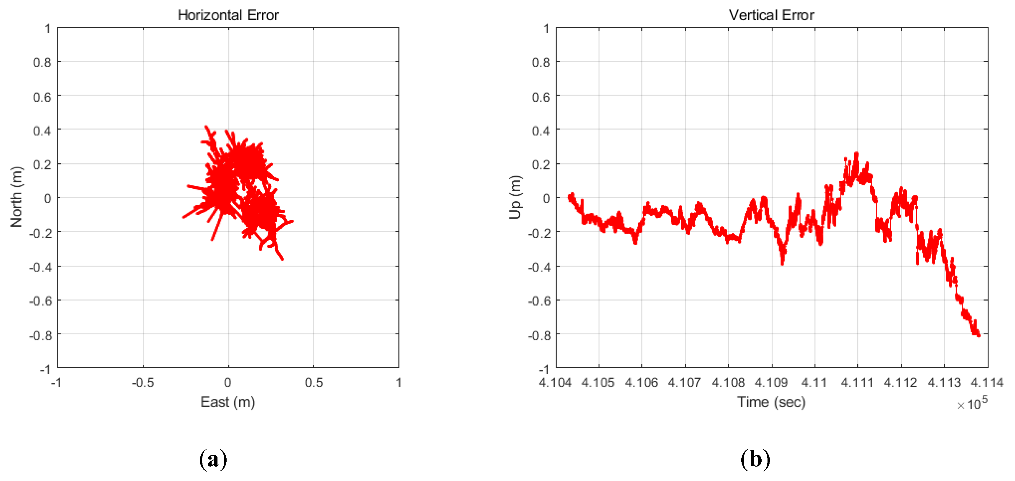
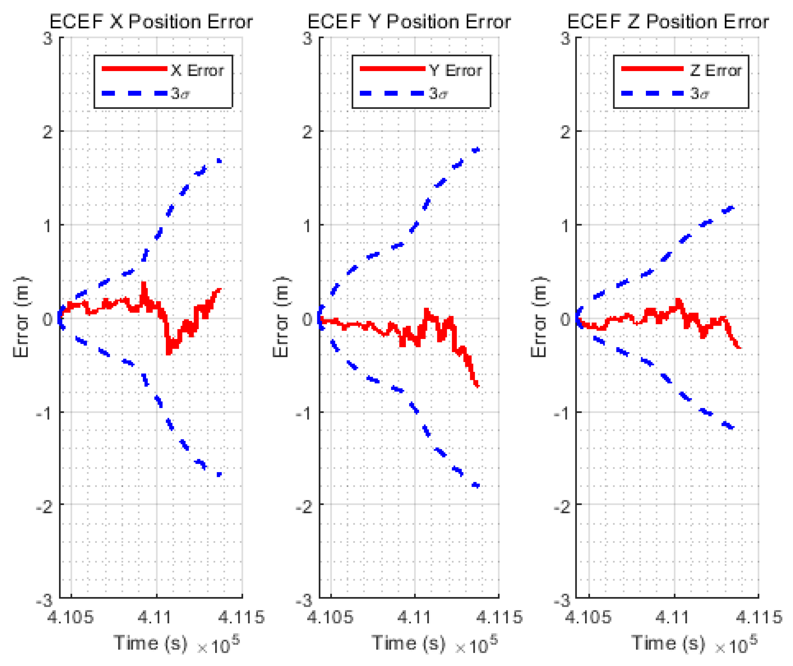
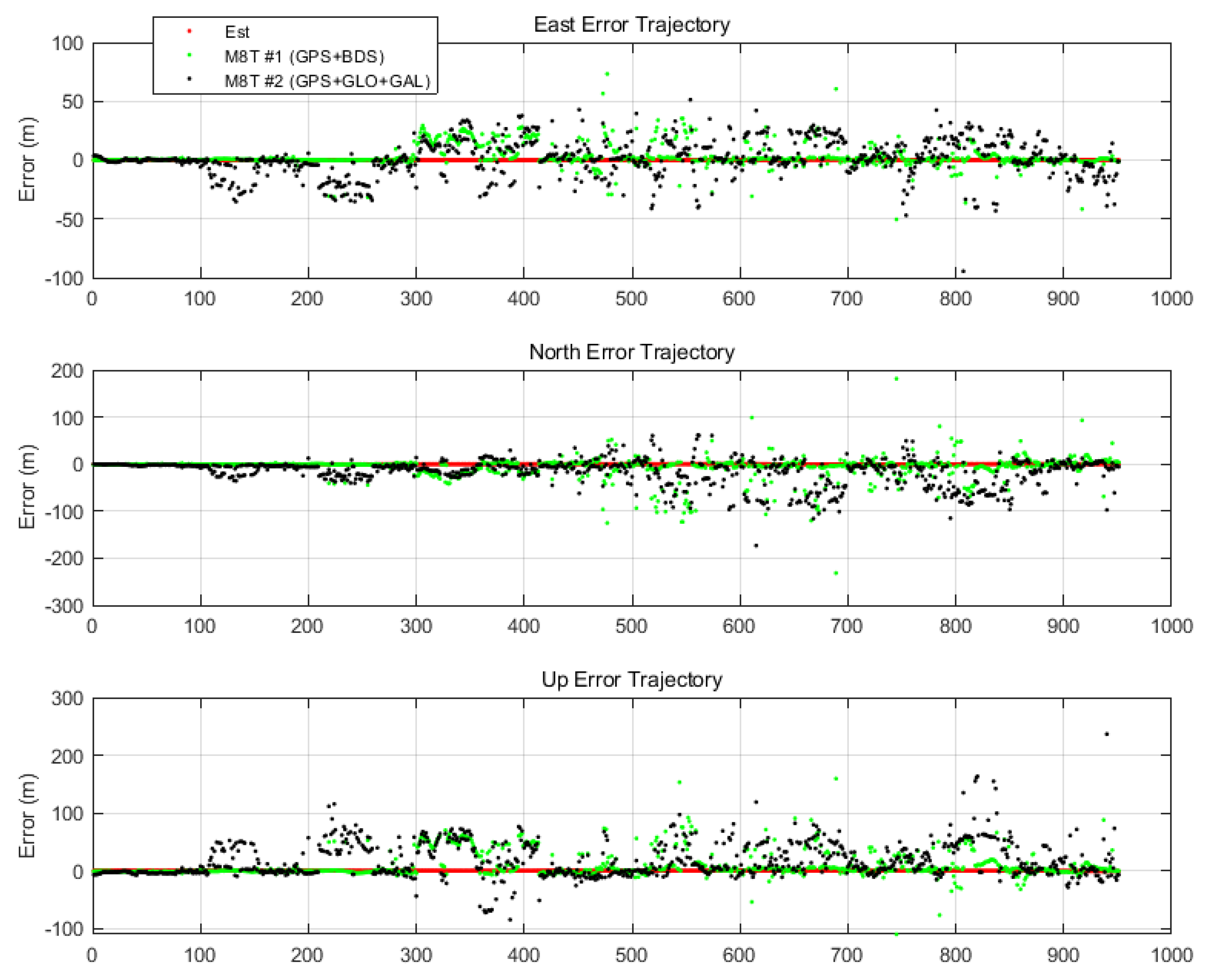
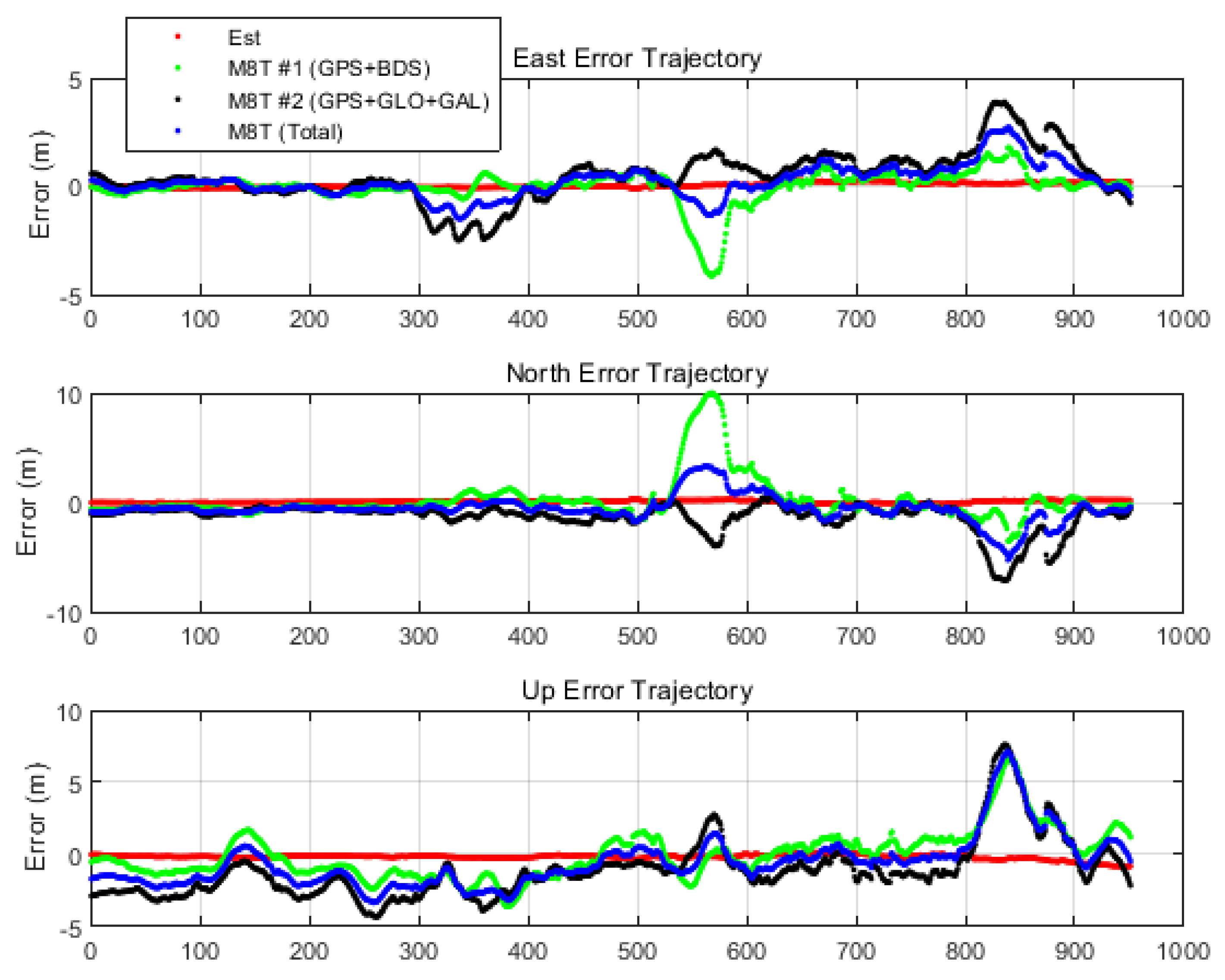
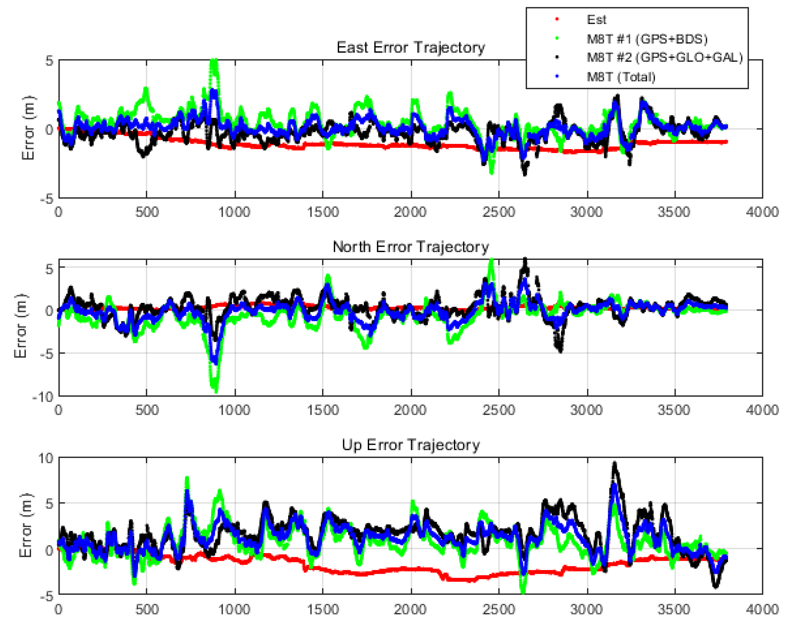
3.2. Test Results
4. Conclusions
Author Contributions
Funding
Conflicts of Interest
References
- Rhee, J.H.; Seo, J. Low-cost curb detection and localization system using multiple ultrasonic sensors. Sensors 2019, 19, 1389. [Google Scholar] [CrossRef] [Green Version]
- Haala, N.; Peter, M.; Kremer, J.; Hunter, G. Mobile LiDAR mapping for 3D point cloud collection in urban areas—A performance test. Int. Arch. Photogramm. Remote Sens. Spat. Inf. Sci. 2008, 37, 1119–1127. [Google Scholar]
- Huang, A.S.; Moore, D.; Antone, M.; Olson, E.; Teller, S. Finding multiple lanes in urban road networks with vision and lidar. Auton. Robot. 2009, 26, 103–122. [Google Scholar] [CrossRef] [Green Version]
- Kim, K.W.; Jee, G.I. Free-resolution probability distributions map-based precise vehicle localization in urban areas. Sensors 2020, 20, 1220. [Google Scholar] [CrossRef] [Green Version]
- González-Jorge, H.; Díaz-Vilariño, L.; Lorenzo, H.; Arias, P. Evaluation of driver visibility from mobile lidar data and weather conditions. Int. Arch. Photogramm. Remote Sens. Spat. Inf. Sci. ISPRS Arch. 2016, 41, 577–582. [Google Scholar] [CrossRef]
- Shin, Y.H.; Lee, S.; Seo, J. Autonomous safe landing-area determination for rotorcraft UAVs using multiple IR-UWB radars. Aerosp. Sci. Technol. 2017, 69, 617–624. [Google Scholar] [CrossRef]
- Li, T.; Petovello, M.G.; Lachapelle, G.; Basnayake, C. Performance Evaluation of Ultra-tight Integration of GPS/Vehicle Sensors for Land Vehicle Navigation. In Proceedings of the 22nd International Technical Meeting of the Satellite Division of The Institute of Navigation (ION GNSS 2009), Savannah, GA, USA, 22–25 September 2009; pp. 1785–1796. [Google Scholar]
- Cai, C.; Gao, Y. Modeling and assessment of combined GPS/GLONASS precise point positioning. GPS Solut. 2013, 17, 223–236. [Google Scholar] [CrossRef]
- Honda, M.; Murata, M.; Mizukura, Y. Development and Assessment of GPS Precise Point Positioning Software for Land Vehicular Navigation. SICE e-J. 2007, 6, 77–84. [Google Scholar]
- Yoon, H.; Seok, H.; Lim, C.; Park, B. An Online SBAS Service to Improve Drone Navigation Performance in High-Elevation Masked Areas. Sensors 2020, 20, 3047. [Google Scholar] [CrossRef] [PubMed]
- Groves, P.D.; Adjrad, M. Likelihood-based GNSS positioning using LOS/NLOS predictions from 3D mapping and pseudoranges. GPS Solut. 2017, 21, 1805–1816. [Google Scholar] [CrossRef] [Green Version]
- Rispoli, F.; Enge, P.; Neri, A.; Senesi, F.; Ciaffi, M.; Razzano, E. GNSS for rail automation & driverless cars: A give and take paradigm. In Proceedings of the 31st International Technical Meeting of the Satellite Division of the Institute of Navigation (ION GNSS+ 2018), Miami, FL, USA, 24–28 September 2018; pp. 1468–1482. [Google Scholar]
- Maddern, W.; Pascoe, G.; Gadd, M.; Barnes, D.; Yeomans, B.; Newman, P. Real-time Kinematic Ground Truth for the Oxford RobotCar Dataset. arXiv 2020, arXiv:2002.10152. [Google Scholar]
- Elsheikh, M.; Abdelfatah, W.; Nourledin, A.; Iqbal, U.; Korenberg, M. Low-cost real-time PPP/INS integration for automated land vehicles. Sensors 2019, 19, 4896. [Google Scholar] [CrossRef] [PubMed] [Green Version]
- Soon, B.K.H.; Scheding, S.; Lee, H.K.; Lee, H.K.; Durrant-Whyte, H. An approach to aid INS using time-differenced GPS carrier phase (TDCP) measurements. GPS Solut. 2008, 12, 261–271. [Google Scholar] [CrossRef]
- Han, S.; Wang, J. Integrated GPS/INS navigation system with dual-rate Kalman Filter. GPS Solut. 2012, 16, 389–404. [Google Scholar] [CrossRef]
- Wendel, J.; Trommer, G.F. Tightly coupled GPS/INS integration for missile applications. Aerosp. Sci. Technol. 2004, 8, 627–634. [Google Scholar] [CrossRef]
- Kim, Y.; Song, J.; Ho, Y.; Park, B.; Kee, C. Optimal Selection of an Inertial Sensor for Cycle Slip Detection Considering Single-frequency RTK/INS Integrated Navigation. Trans. Jpn. Soc. Aeronaut. Space Sci. 2016, 59, 205–217. [Google Scholar] [CrossRef] [Green Version]
- Kim, J.; Kim, Y.; Song, J.; Kim, D.; Park, M.; Kee, C. Performance Improvement of Time-Differenced Carrier Phase Measurement-Based Integrated GPS/INS Considering Noise Correlation. Sensors 2019, 19, 3084. [Google Scholar] [CrossRef] [Green Version]
- Kim, J.; Kee, C. A low-cost high-precision vehicle navigation system for urban environment using time differenced carrier phase measurements. In Proceedings of the 2020 International Technical Meeting of The Institute of Navigation, San Diego, CA, USA, 21–24 January 2020; pp. 597–611. [Google Scholar]
- Groves, P.D.; Jiang, Z.; Wang, L.; Ziebart, M.K. Intelligent urban positioning using multi-constellation GNSS with 3D mapping and NLOS Signal detection. In Proceedings of the 25th International Technical Meeting of the Satellite Division of the Institute of Navigation, Nashville, TN, USA, 17–21 September 2012; pp. 458–472. [Google Scholar]
- Groves, P.D. How Does Non-Line-of-Sight Reception Differ from Multipath Interference? Insid. GNSS 2013, 8, 40–42. [Google Scholar]
- Ding, W.; Wang, J. Precise velocity estimation with a stand-alone GPS receiver. J. Navig. 2011, 64, 311–325. [Google Scholar] [CrossRef] [Green Version]
- Freda, P.; Angrisano, A.; Gaglione, S.; Troisi, S. Time-differenced carrier phases technique for precise GNSS velocity estimation. GPS Solut. 2015, 19, 335–341. [Google Scholar] [CrossRef]
- Brown, R.; Hwang, P. Introduction to Random Signals and Applied Kalman Filtering with MatLab Excercises Fourth Edition; Wiley: Hoboken, NJ, USA, 2012; ISBN 9780470609699. [Google Scholar]
- Rhee, I.; Abdel-Hafez, M.F.; Speyer, J.L. Observability of an integrated GPS/INS during maneuvers. IEEE Trans. Aerosp. Electron. Syst. 2004, 40, 526–535. [Google Scholar] [CrossRef]
- Karaim, M.O.; Karamat, T.B.; Noureldin, A.; Tamazin, M.; Atia, M.M. Real-time cycle-slip detection and correction for land vehicle navigation using Inertial aiding. In Proceedings of the 26th International Technical Meeting of the Satellite Division of the Institute of Navigation (ION GNSS+ 2013), Nashville, TN, USA, 16–20 September 2013; pp. 1290–1298. [Google Scholar]
- Bisnath, S. Efficient, Automated cycle-slip correction of dual-frequency kinematic GPS data. In Proceedings of the 13th International Technical Meeting of the Satellite Division of the Institute of Navigation (ION GPS 2000), Salt Lake City, UT, USA, 19–22 September 2000; pp. 145–154. [Google Scholar]
- Park, B. A Study on Reducing Temporal and Spatial Decorrelation Effect in GNSS Augmentation System: Consideration of the Correction Message Standardization. Ph.D. Thesis, Seoul National University, Seoul, Korea, 2008. [Google Scholar]
- Du, S.; Gao, Y. Inertial aided cycle slip detection and identification for integrated PPP GPS and INS. Sensors 2012, 12, 14344–14362. [Google Scholar] [CrossRef] [PubMed] [Green Version]
- Cai, C.; Gao, Y. A combined GPS/GLONASS navigation algorithm for use with limited satellite visibility. J. Navig. 2009, 62, 671–685. [Google Scholar] [CrossRef]
- Tools, G.U.I. Inertial Explorer ® Version History. Available online: https://portal.hexagon.com/public/Novatel/assets/Documents/Waypoint/InertialExplorerNewFeatures (accessed on 5 April 2020).


| RMS 1 | TDCP/INS (Proposed) | Ublox M8T #1 | Ublox M8T #2 | Ublox M8T #1, #2 Average |
|---|---|---|---|---|
| East | 0.11 m | 0.80 m | 1.23 m | 0.78 m |
| North | 0.13 m | 2.03 m | 1.87 m | 1.31 m |
| Up | 0.24 m | 1.67 m | 2.31 m | 1.85 m |
| RMS 1 | TDCP/INS (Proposed) | Ublox M8T #1 | Ublox M8T #2 | Ublox M8T #1, #2 Average |
|---|---|---|---|---|
| East | 0.27 m | 4.14 m | 3.89 m | 2.73 m |
| North | 0.34 m | 10.04 m | 7.13 m | 5.25 m |
| Up | 0.81 m | 6.88 m | 7.60 m | 7.26 m |
| RMS 1 | TDCP/INS (Proposed) | Ublox M8T #1 | Ublox M8T #2 | Ublox M8T #1, #2 Average |
|---|---|---|---|---|
| East | 1.18 m | 1.06 m | 0.82 m | 0.68 m |
| North | 0.33 m | 1.77 m | 1.30 m | 1.20 m |
| Up | 1.89 m | 1.84 m | 2.45 m | 1.90 m |
| RMS 1 | TDCP/INS (Proposed) | Ublox M8T #1 | Ublox M8T #2 | Ublox M8T #1, #2 Average |
|---|---|---|---|---|
| East | 1.73 m | 4.97 m | 3.37 m | 2.77 m |
| North | 0.89 m | 9.61 m | 6.01 m | 6.32 m |
| Up | 3.47 m | 7.73 m | 9.32 m | 6.99 m |
© 2020 by the authors. Licensee MDPI, Basel, Switzerland. This article is an open access article distributed under the terms and conditions of the Creative Commons Attribution (CC BY) license (http://creativecommons.org/licenses/by/4.0/).
Share and Cite
Kim, J.; Park, M.; Bae, Y.; Kim, O.-J.; Kim, D.; Kim, B.; Kee, C. A Low-Cost, High-Precision Vehicle Navigation System for Deep Urban Multipath Environment Using TDCP Measurements. Sensors 2020, 20, 3254. https://doi.org/10.3390/s20113254
Kim J, Park M, Bae Y, Kim O-J, Kim D, Kim B, Kee C. A Low-Cost, High-Precision Vehicle Navigation System for Deep Urban Multipath Environment Using TDCP Measurements. Sensors. 2020; 20(11):3254. https://doi.org/10.3390/s20113254
Chicago/Turabian StyleKim, Jungbeom, Minhuck Park, Yonghwan Bae, O-Jong Kim, Donguk Kim, Bugyeom Kim, and Changdon Kee. 2020. "A Low-Cost, High-Precision Vehicle Navigation System for Deep Urban Multipath Environment Using TDCP Measurements" Sensors 20, no. 11: 3254. https://doi.org/10.3390/s20113254