PM2.5 Concentration Estimation Based on Image Processing Schemes and Simple Linear Regression
by
Jiun-Jian Liaw
1, 
Yung-Fa Huang
1,
Cheng-Hsiung Hsieh
2,*,
Dung-Ching Lin
1 and
Chin-Hsiang Luo
3 1
Department of Information and Communication Engineering, Chaoyang University of Technology, 168, Jifeng E. Rd., Wufeng District, Taichung 413310, Taiwan
2
Department of Computer Science and Information Engineering, Chaoyang University of Technology, 168, Jifeng E. Rd., Wufeng District, Taichung 413310, Taiwan
3
Department of Safety, Health and Environmental Engineering, Hungkuang University, 1018, Sec. 6, Taiwan Blvd., Shalu District, Taichung 433304, Taiwan
*
Author to whom correspondence should be addressed.
Sensors 2020, 20(8), 2423; https://doi.org/10.3390/s20082423
Submission received: 28 February 2020
/
Revised: 15 April 2020
/
Accepted: 23 April 2020
/
Published: 24 April 2020
(This article belongs to the Special Issue Selected Papers from the First International Symposium on Future ICT (Future-ICT 2019) in Conjunction with 4th International Symposium on Mobile Internet Security (MobiSec 2019))
Abstract
:Fine aerosols with a diameter of less than 2.5 microns (PM2.5) have a significant negative impact on human health. However, their measurement devices or instruments are usually expensive and complicated operations are required, so a simple and effective way for measuring the PM2.5 concentration is needed. To relieve this problem, this paper attempts to provide an easy alternative approach to PM2.5 concentration estimation. The proposed approach is based on image processing schemes and a simple linear regression model. It uses images with a high and low PM2.5 concentration to obtain the difference between these images. The difference is applied to find the region with the greatest impact. The approach is described in two stages. First, a series of image processing schemes are employed to automatically select the region of interest (RoI) for PM2.5 concentration estimation. Through the selected RoI, a single feature is obtained. Second, by employing the single feature, a simple linear regression model is used and applied to PM2.5 concentration estimation. The proposed approach is verified by the real-world open data released by Taiwan’s government. The proposed scheme is not expected to replace component analysis using physical or chemical techniques. We have tried to provide a cheaper and easier way to conduct PM2.5 estimation with an acceptable performance more efficiently. To achieve this, further work will be conducted and is summarized at the end of this paper.
1. Introduction
Air pollution has been reported to significantly affect human health [1], causing issues such as premature death, bronchitis, asthma, cardiovascular disease, and lung cancer [2]. Pollutants in the air include CO, NO2, and particulate matter. Among them, particulate matter with a diameter of less than 2.5 microns (PM2.5) is a key component which severely affects human health in many ways. For example, PM2.5 aerosols are able to directly enter the lungs through the respiratory tract and affect a person’s health [3]. According to the World Health Organization report, more than 90% of the world’s population inhales large amounts of pollutants every day, which results in approximately seven million deaths each year [4]. Consequently, PM2.5 concentration estimation is required and has become an important concern for human health [5,6].
Many techniques have been developed to measure the PM2.5 concentration, such as the filter-based gravimetric method [7], tapered element oscillating microbalance method [8], beta attenuation monitoring method [9], optical analysis method [10,11], and black smoke measurement [12]. These methods require expensive instruments and professional operations. Some more comprehensive methods analyze the relationship between human activities and PM2.5 by satellite and big data [13,14]. However, satellite and big data are not available to the common user. Therefore, a simple and effective method should be sought for PM2.5 concentration estimation.
In urban environments, researchers have developed low-cost sensors. These sensors are widely deployed throughout the city to monitor the PM2.5 concentration [15]. Although one sensor is low in cost, it is not effective when widely deployed in a city requiring many sensors. The portable PM2.5 sensor can be used to monitor the PM2.5 concentration at different locations [16]. The portable device reduces the cost of employing a large number of sensors, but requires more manpower to move the sensors. Optical sensors, such as TEOM 1400a analyzer, SDS011 (Nova Fitness, Jinan, China), ZH03A (Winsen, Zhengzhou, China), PMS7003 (Plantower, Beijing China), and OPC-N2 (Alphasense, Braintree, UK), have been introduced to monitor PM2.5 [17]. However, these optical sensors are more expensive than ordinary cameras. Since a camera is installed on the top floor of environmental monitoring stations in Taiwan, using the camera to estimate PM2.5 is a simpler and more effective approach than employing extra devices.
It should be noted that air pollution is usually characterized by a poor visibility due to light scattering, such as Rayleigh scattering and Mie scattering, caused by the interaction between light and airborne particles [18]. In other words, the visibility is reduced, as a large amount of aerosol pollution scatter the atmospheric light [19], and vice versa. In previous decades, some researchers proposed methods to estimate the visibility through image processing schemes [20,21]. Recently, an expensive digital camera was used to take high-quality photos for visibility estimation [22]. These studies have shown that image processing schemes can be applied to visibility estimation. Furthermore, it was reported that the PM2.5 concentration is related to visibility reduction [23]. However, these studies did not develop image processing technologies to estimate the PM2.5 concentration. Therefore, it gives us hope that the PM2.5 concentration may be estimated through image processing schemes.
The rapid development of computers, algorithms, and artificial intelligence has meant that image processing methods using machine learning have been widely applied. The main advantage of using machine learning is that it requires training and does not require defining too many features. Two types of the training-based algorithms are neural network methods [24] and linear regression schemes [25]. The neural network methods require a very fast and expensive graphics processing unit [26]. By contrast, compared to neural network methods, the estimation of spatial variations by linear regression could be performed by a consumer computer, as economical and predictive performance were both acceptable [27]. Nowadays, high-quality images can be taken by a commercial digital camera. This facilitates PM2.5 concentration estimation by image processing schemes.
In order to understand which features can affect PM2.5 concentrations when using image processing methods, previous research has pointed out that the PM2.5 concentrations may affect image characteristics, including the distance, hazy model, entropy, contrast, sky color, and solar zenith angle. It was found that the distance is the feature that has the most influence [28]. This is consistent with the definition of visibility, and a previous study has also shown that visibility can be estimated using high-frequency information from an image [22]. The region of interest (RoI) has also been manually selected to estimate PM2.5 concentrations [28]. However, the estimation performance might be degraded because of such a manually selected RoI. Besides, the computational cost might not be cheap, since a support vector regression model with several features was involved in the estimation. To solve these problems, this paper presents an approach to PM2.5 concentration estimation, where only a single feature is used and simple linear regression is employed as an estimator. The main contribution of the proposed approach is to use a series of image processing schemes in PM2.5 concentration estimation where the images are taken by a consumer camera. It provides a valuable alternative to estimating PM2.5 concentration. The main aims of this image-based approach are as follows: (i) to automatically locate the RoI to replace the manual selection of Liu’s work [28]; (ii) to use a single feature for linear regression instead of multiple features in PM2.5 concentration estimation, with an acceptable performance; and (iii) to provide a cheaper alternative method with a camera for estimating the PM2.5 concentration. This paper is organized as follows. The proposed approach is described in Section 2. In Section 3, real-world data is given to verify the proposed approach. Finally, a conclusion is made in Section 4.
2. The Proposed Approach
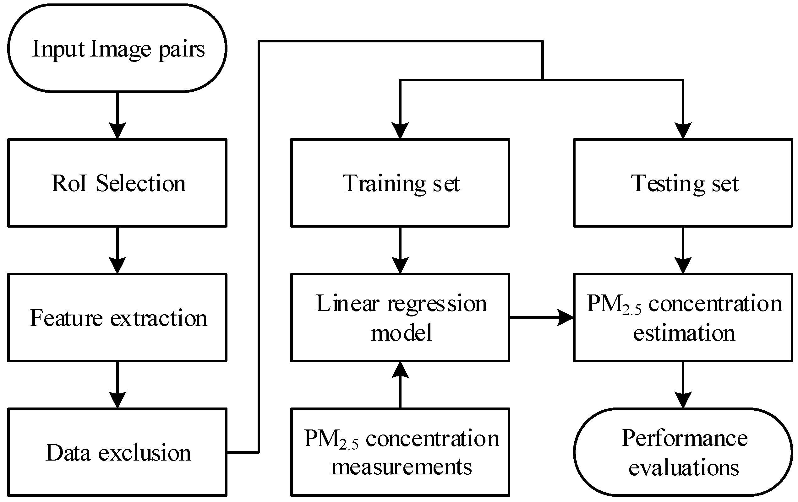
There are two stages involved in the proposed approach. In the first stage, a series of image processing schemes are employed to automatically locate the region of interest (RoI) to extract a single feature, which is required in the following stage for PM2.5 concentration estimation. In the second stage, a simple linear regression model is used with the training data, which contains pairs of the single feature obtained through the selected RoI and the actual PM2.5 concentration measurement. The simple linear regression model is then used in PM2.5 concentration estimation with the testing data. The estimated PM2.5 concentration is compared with the actual value and evaluated by performance indices. An overall block diagram for the proposed approach is depicted in Figure 1. The details of the proposed approach are described in the following sections. The proposed automatic RoI selection approach is described in Section 2.1, the simple linear regression model is given in Section 2.2, and three performance indices employed to assess the proposed approach are given in Section 2.3.
2.1. Automatic RoI Selection
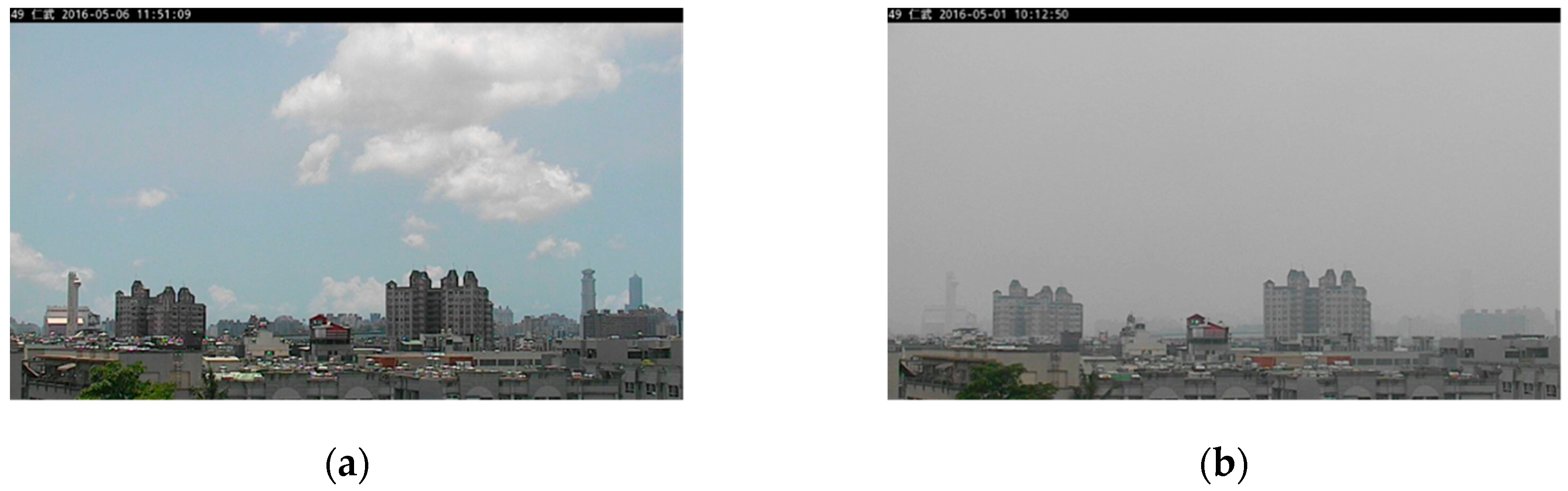
It should be noted that not all parts of an image are strongly related to the PM2.5 concentration. Therefore, selecting an appropriate RoI to estimate the PM2.5 concentration is an important step for the successful application of the proposed approach. It is known that some details in the image will be blurred when the PM2.5 concentration is high, compared to when there is a low PM2.5 concentration. In other words, the pixel value of the images with a high and low PM2.5 concentration is different. This also illustrates that not every feature has a good correlation with the PM2.5 concentration. It motivates us to use the differences in image pairs of low and high PM2.5 concentrations in automatic RoI selection. A flowchart of the proposed automatic RoI selection is depicted in Figure 2. A pair of images, shown in Figure 3a,b, are given to demonstrate how the proposed automatic RoI selection works. Given a pair of images of low and high PM2.5 concentrations, both images are converted into gray-level images. The image of a low PM2.5 concentration is denoted as I1 and the one with a high PM2.5 concentration is denoted as I2. A series of image processing steps to determine the final RoI is described in the following.
2.1.1. Sobel Edge Detection
As the first step, Sobel edge detection is applied to the image pair, I1 and I2, to extract the high-frequency components [29]. In Sobel edge detection, the gradients used in this approach for the x-axis and y-axis, respectively, are denoted as Gx and Gy, and given as
where a 3 × 3 mask is employed. The final magnitude Gxy is calculated as
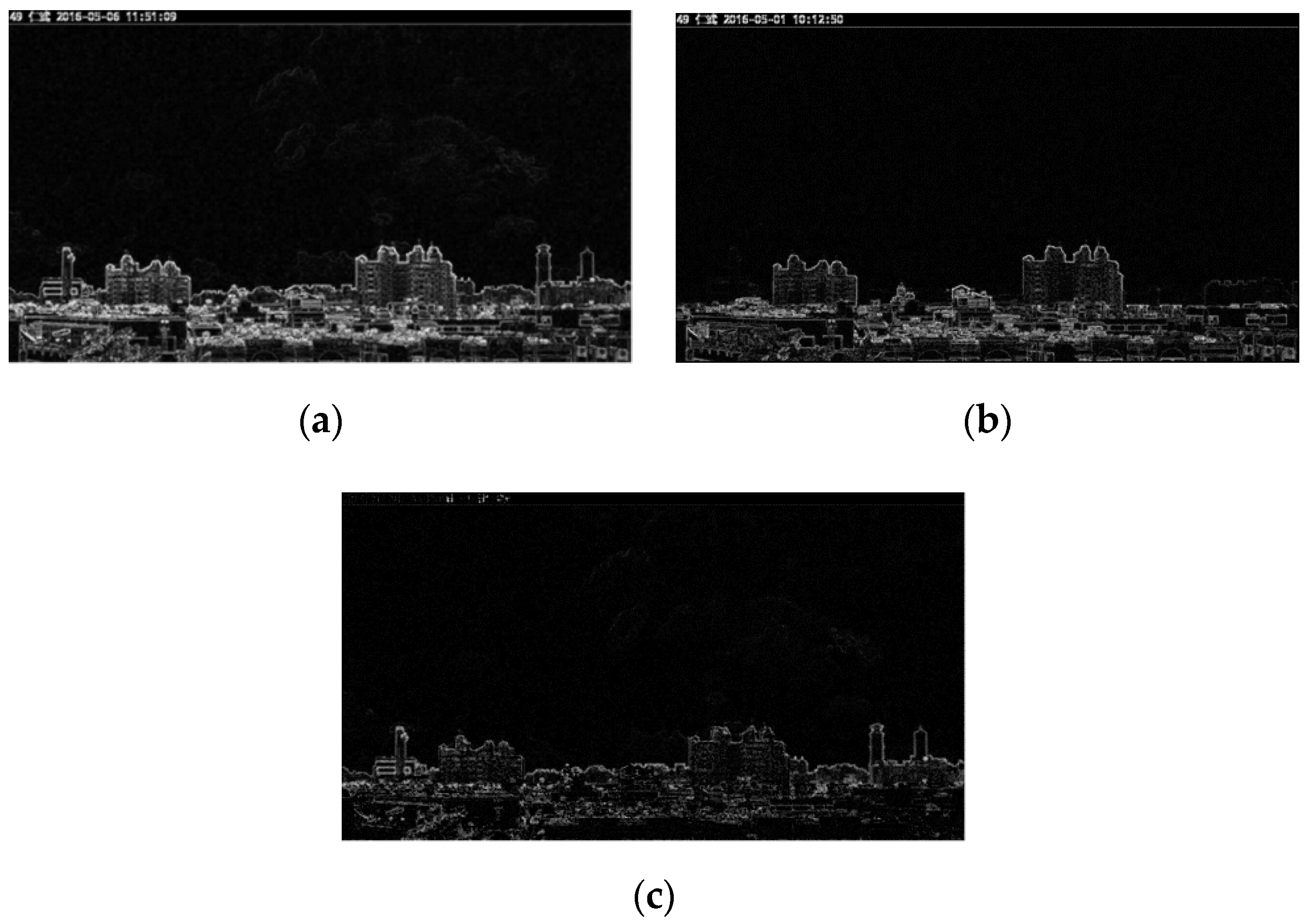
The images produced by Sobel edge detection are denoted as I1,s and I2,s, and are shown in Figure 4a,b, respectively. In Figure 4, one can see that the low concentration image I1, after Sobel edge detection, has more details than I2. This shows that more high-frequency components are contained in I1,s than I2,s. The edge detection results of Figure 3a,b are shown in Figure 4a,b, respectively. We can see that two buildings on the right of Figure 3a do not appear in Figure 3b. This is because the PM2.5 concentration of Figure 3b is higher than that of Figure 3a. This means that the edges of the two buildings are invisible in Figure 4b. The difference of Figure 4a,b is shown in Figure 4c. The results show that the PM2.5 concentration has a significant effect on the high frequency components of images.
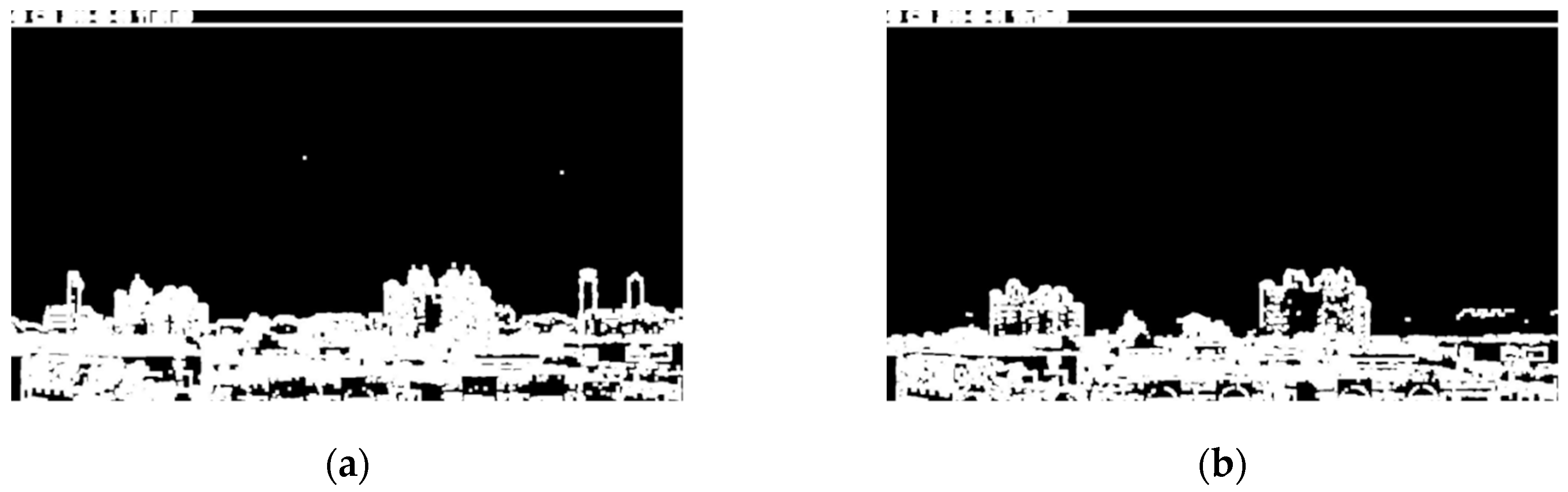
2.1.2. Otsu Thresholding
After Sobel edge detection, Otsu thresholding [30] is applied to the two images in Figure 4 to obtain binary images. In Otsu thresholding, the pixels in an image are separated into two groups based on the histogram. By employing statistical properties, the optimal threshold, where the variance of each group is minimized and the variance between two groups is maximized, is determined. In Otsu thresholding, the weighted sum of the variance between two groups is found as
where and represent the variance of each group and are the weights of two groups separated by the threshold t, respectively. The weights and are obtained, respectively, as
and
where p is the probability of the pixel value i and L is the number of gray levels. The variance between two groups is given as
where is the variance of the whole image. Equation (6) can be transformed into
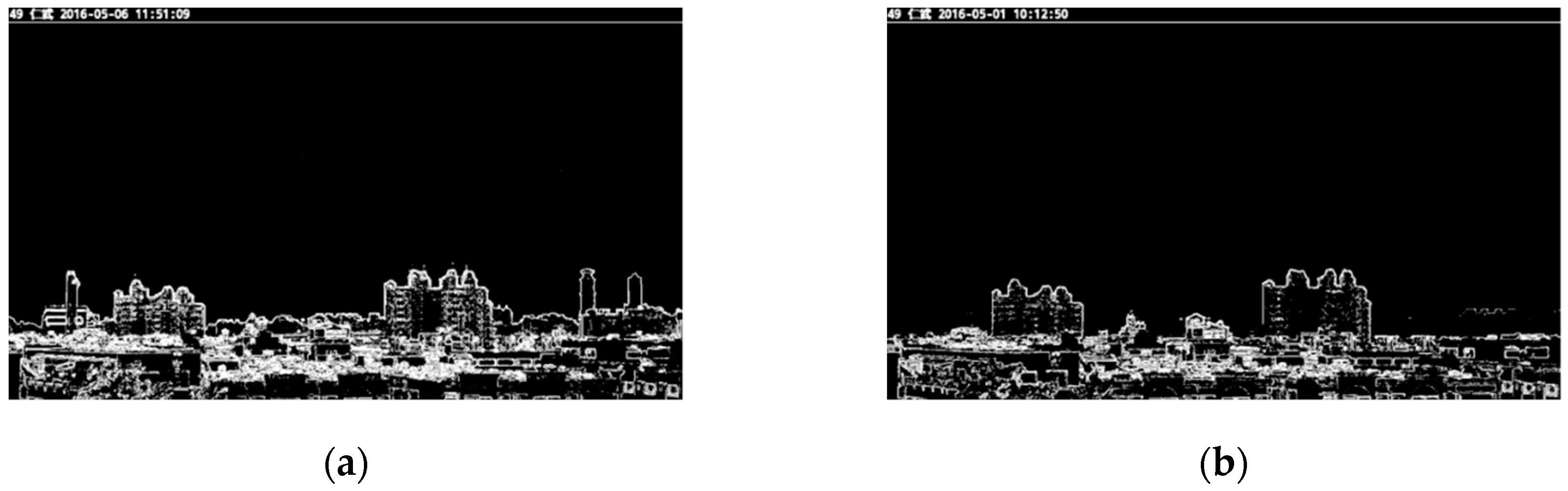
where and are the means of two groups separated by threshold t. The optimal threshold is then found with t, which maximizes in Equation (7). The images I1,s and I2,s after Otsu thresholding, are denoted as I1,so and I2,so and shown in Figure 5a and Figure 5b, respectively.
2.1.3. Morphological Dilation
Using the obtained binary images, I1,so and I2,so, shown in Figure 5, morphological dilation is applied to expand boundaries and to connect neighborhood pixels. The degree of expansion depends on the size of structuring elements. The equation employed for morphological dilation is given below:
where A is the image to be processed and B represents the structuring elements.
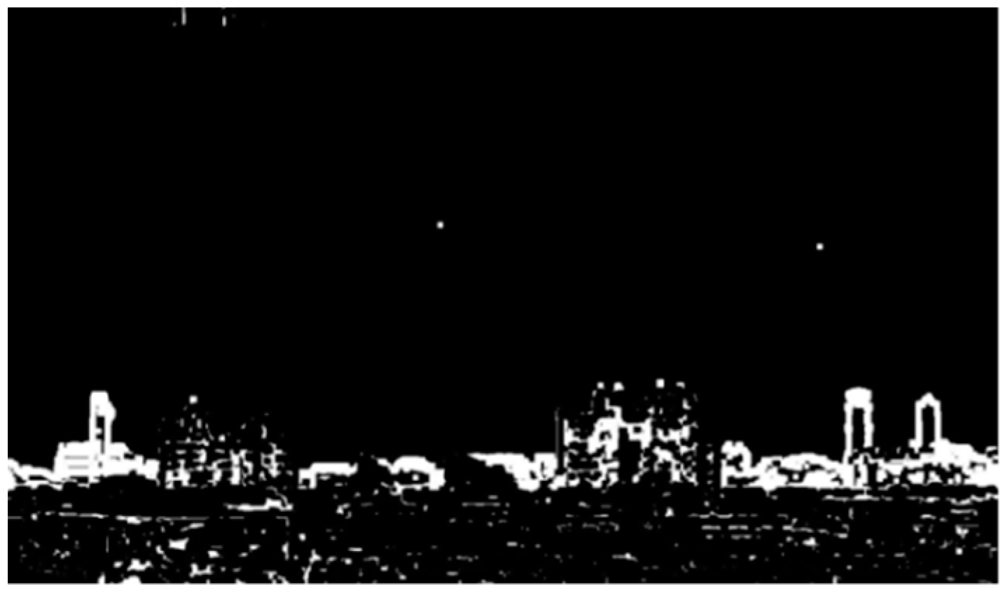
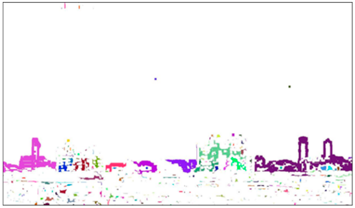
2.1.4. Image Subtraction and Labeling
In this step, image subtraction is used to obtain the difference image for I1,som and I2,som in Figure 6. Then, a labeling scheme is employed to identify connected pixels. The difference image for I1,som and I2,som is shown in Figure 7, denoted as Id, where pixels with the same value in the image pair are eliminated and those with different pixel values remain in a white color. In order to distinguish whether pixels are connected, a labeling scheme [31] is applied to mark the connected pixels by colors. The connected neighborhood pixels are marked with the same color. After labeling, the resulting image, denoted as Idl, is as shown in Figure 8. Finally, the labeled regions with the top three largest numbers of pixels are considered as candidate regions of interest.
2.1.5. Selected RoI in the Given Pair of Images
Now, the red flow path shown in Figure 2 will be described. The difference image, denoted as Isd, for I1,s and I2,s is obtained by image subtraction. Then, the three candidate regions of interest and the difference image Isd are overlapped to select the pixels in the candidate regions of interest. Next, the averages of pixel values in each candidate region of interest are calculated. Then, the RoI with the highest average is determined as the final RoI in the given pair of images, I1 and I2. This completes the process of automatic RoI selection given in Figure 2 for the given pair of images.
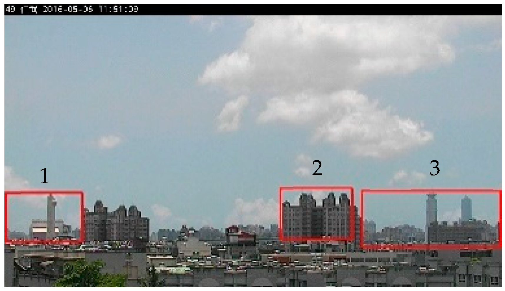
2.1.6. Final RoI Determination
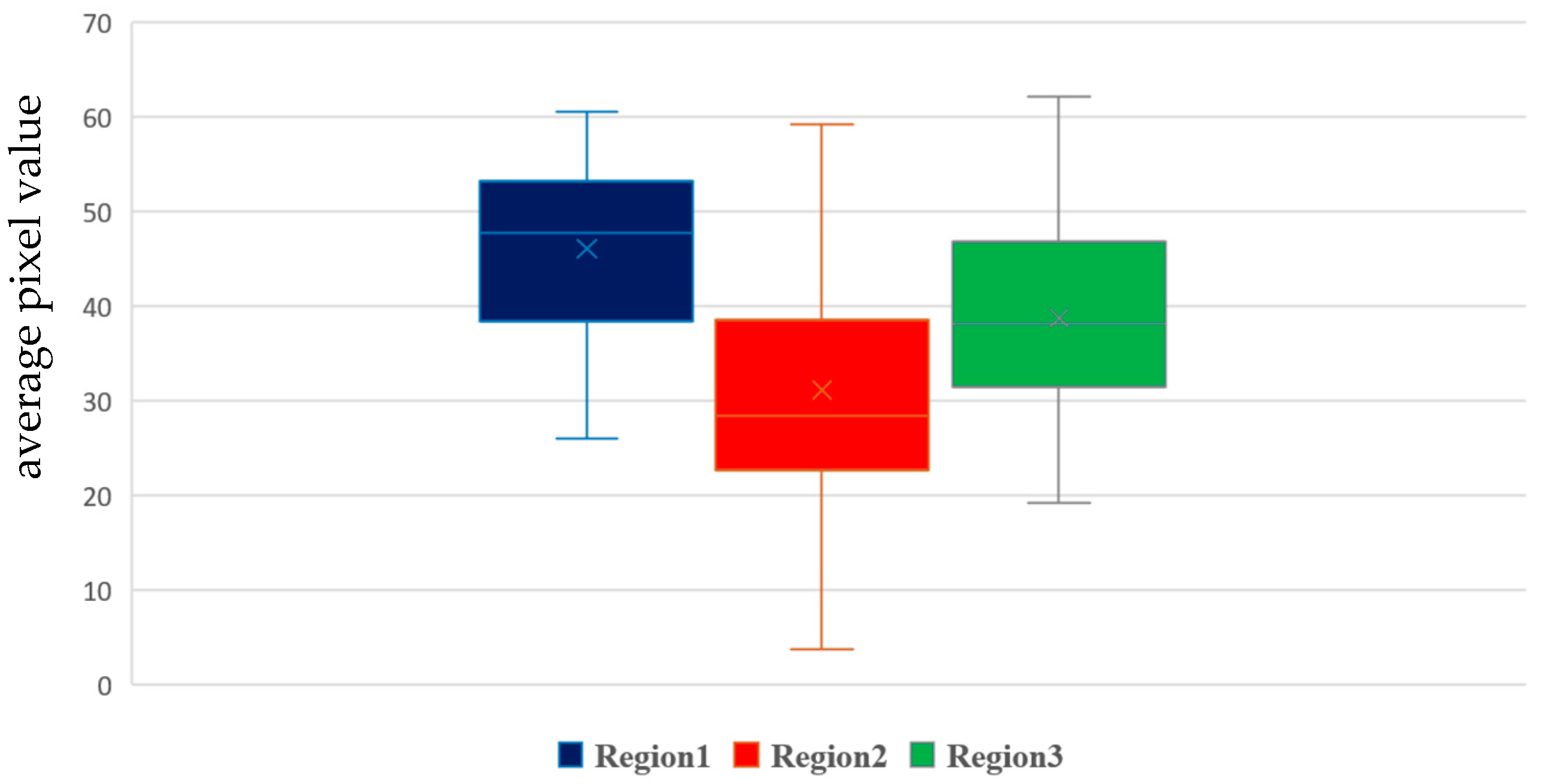
It needs to be pointed out that the image pair given above is just an example provided to show the process of the proposed automatic RoI selection. In practice, in automatic RoI selection, 30 images with a low PM2.5 concentration (≤) and 120 images with a high PM2.5 concentration (≥) are randomly selected from the training set. In this study, the images with low and high PM2.5 concentrations are paired by combinations. In other words, the 30 × 120 paired images are included in the automatic RoI selection process, as described in Figure 2. By using the averages of 3600 results, the three candidate regions of interest are determined, as shown in Figure 9. The box plot given in Figure 10 shows the range of average pixel values in each candidate RoI. Since Region 1 has the highest average value, it is selected as the final RoI to estimate the PM2.5 concentration. The average pixel value within the final RoI will be used as the only single feature for the following simple linear regression model in the proposed approach.
2.2. Simple Linear Regression Model
A simple linear regression model, which is a statistical analysis scheme [25], will be used to estimate the PM2.5 concentration in the proposed approach. is the average pixel value within the final data and is the corresponding PM2.5 concentration measurement in the training data (where subscript i denotes the ith sample). It is assumed that these two sequences of data have a linear relation, shown as
where and are coefficients to be determined. denotes an estimate of (corresponding PM2.5 concentration). The estimation error between and is given as
Employing the least squares algorithm to minimize the estimation error, coefficients and can be found as
and
where N is the number of samples. Once the simple linear regression model is obtained, it is employed to estimate the PM2.5 concentration with the testing data.
2.3. Performance Indices
Inherently, image-based method cannot analyze the ingredients in the air, as in previous works, thus it is hard to define a parameter to show the performance by error. Instead, three overall performance indices are used to evaluate the proposed approach. The first one is the root mean square error (RMSE). It is used to show the error between the recorded value and the estimated value of the proposed method. RMSE is calculated as
where and are the true and estimated PM2.5 concentrations, respectively. The second performance index is R squared (R2), which has also been used in previous work [28], and is employed to show the correlation between estimated results and measured values. It is defined as
where is the mean of . R2 indicates the linearity between and . When it is linear, R2 = 1. The third index is F-test, which is the test statistic for an F-distribution under the null hypothesis [32], where the p-value indicates the statistical significance; that is, it determines whether the result is beyond chance or not. The p-value will be used as an indicator of statistical significance in the following experiments.
3. Experimental Results
In this section, the proposed approach is verified by a real-world data set, which is described later in Section 3.1. Then, the results without and with unreliable data exclusion are shown in Section 3.2 and Section 3.3, respectively.
3.1. Experimental Data Sets
In the experiments, the images were taken from Renwu Environmental Monitoring Station, Kaohsiung City, Taiwan. A consumer camera was set up at the station and took one image every ten minutes during the period of 7:00 AM to 5:00 PM. In total, 10,084 images were collected from May to October 2016. We did not exclude sampled images of sunny or rainy days. The image data were divided into training and testing data, of which the proportions were 60% and 40%, respectively. The images shown in Figure 3a,b are examples taken from the data set. Furthermore, the hourly PM2.5 concentration and relative humidity (RH) in the corresponding area were obtained from the open data released by the Environmental Protection Administration, Executive Yuan, Taiwan [33]. Using the data, a simple linear regression model was obtained and used to estimate the PM2.5 concentration by employing the proposed approach.
3.2. Results with All Data
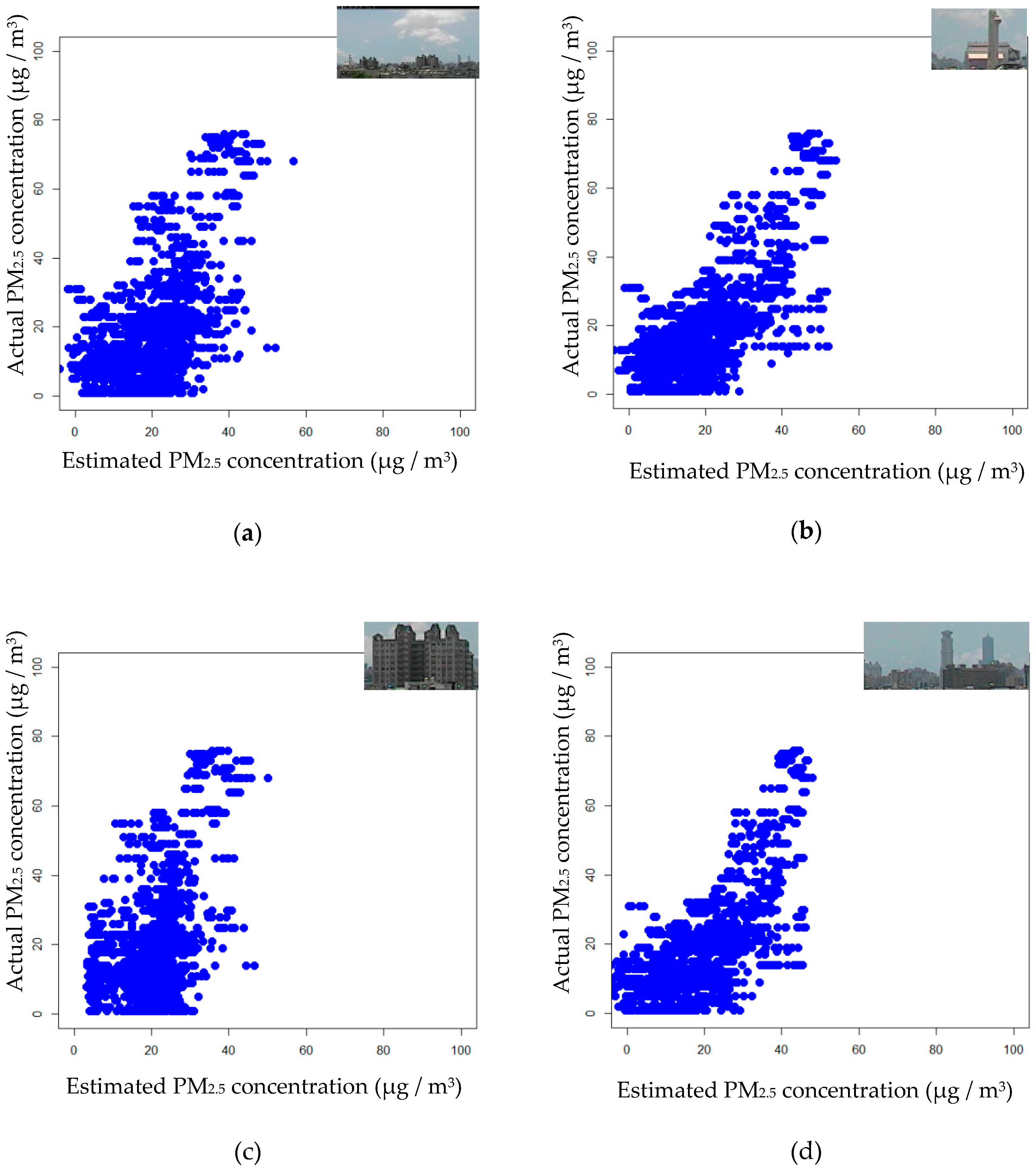
In this experiment, all of the data set, including 10,084 images, was used. As described in Section 2, three candidate regions of interest were automatically selected and the final RoI was determined by the highest average pixel value among the three candidate regions of interest. Besides, the average pixel value in the final RoI was used as the only single feature. To compare the estimation performances for the whole image, Region 1, Region 2, and Region 3 are presented in Figure 11a–d, which show scattering plots for each case, where the region under consideration is shown in the upper right corner. The three performance indices with all data are displayed in Table 1. Table 1 indicated that Region 1 had a better performance than the other cases. Besides, all results were statistically significant in the F-test. In the case with all data, the highest R2 = 0.41, which was achieved by Region 1. One may see that the performance of the whole image case is inferior to those for candidate regions of interest. When Regions 1 to 3 are considered, the performance index R2, from high to low, is Region 1, Region 3, and Region 2. The result is consistent with the priority for the proposed automatic RoI selection. In other words, the proposed automatic RoI selection is appropriate for the given data.
3.3. Results with Unreliable Data Exclusion
By conducting experiments, it was observed that two factors may affect the performance of the proposed approach. One is the time difference between the time to take images and the time to measure the PM2.5 concentration. For the data set described in Section 3.1, the images were taken every ten minutes, but the PM2.5 concentration was collected hourly. In other words, six images were related to only one PM2.5 concentration for each hour. When the PM2.5 concentration changes within an hour, it might degrade the estimation performance. To solve this problem, the variance of six images taken in the same hour was calculated. When the variance was greater than 1, the images were considered as unreliable data and discarded.
The other factor seen to affect the performance of the proposed approach was the RH. There are many substances, in addition to PM2.5, in the atmosphere that affect visibility, such as sulfur oxides, nitrogen oxides, carbon monoxide, and water droplets. It has been observed that PM2.5 aerosols are expanded by absorbing water molecules in the air and this affects visibility [34]. It has also been reported that the RH affects PM2.5 concentration estimation [28]. Consequently, the effect of RH on PM2.5 concentration estimation was considered in the proposed approach.
By conducting experiments, we observed that the estimation performance of the proposed approach was significantly degraded when RH ≥ 65%. Consequently, the data was excluded if its corresponding RH ≥ 65%. Moreover, it should be noted that human health is mostly endangered by a higher PM2.5 concentration, instead of a lower one. Consequently, the data with PM2.5 concentrations less than 5 were excluded. By employing the criteria RH ≥ 65% or PM2.5 concentration less than 5, 2361 images were excluded from the given data set. With the consideration of data exclusion, the three performance indices were recorded and are presented in Table 2 for all cases, as in Table 1. As seen in Table 2, Region 1 had a better performance than the other cases, as in Table 1. Moreover, all results were statistically significant in the F-test. When comparing the results presented in Table 1 and Table 2, one can see that the RMSE and R2 were obviously improved in all cases with data exclusion. Additionally, Region 1 exhibited the most improvement. The RMSE was reduced from 11.88 to 8.67, while the R2 increased from 0.41 to 0.73. Again, the results implied that the automatically selected RoI was appropriate in the given example. To sum up, the proposed approach with automatic RoI selection and data exclusion is feasible and has an acceptable performance for PM2.5 concentration estimation. By Table 2, one may observe that the performance of the whole image case is inferior to those for candidate regions of interest, as in Table 1. According to the results, the performances from high to low are Region 1, Region 3, and Region 2, which is consistent with the priority for the proposed automatic RoI selection, as shown in Figure 10. Again, the results have verified the feasibility of the proposed automatic RoI selection scheme in the given experiments.
4. Conclusions
This paper has presented a simple alternative for estimating the PM2.5 concentration in which a series of image processing schemes and simple linear regression are employed. The proposed method uses images with a high and low PM2.5 concentration to obtain the difference between these images. The difference is used to find the RoI. Two main stages are involved in this approach. The first stage includes a series of image processing schemes, which are used to automatically select the final RoI, from which only a single feature is extracted and used in a simple linear regression model. The second stage is employed to find a simple linear regression model with the single feature, by applying the final RoI identified in the first stage. Then, PM2.5 concentration estimation is performed. Using an image data set and an open PM2.5 concentration data set, experiments were conducted to verify the proposed approach. The results indicated that the proposed approach with the automatically selected RoI achieved the best performance, with R2 = 0.73. Although the proposed method is not as direct as chemical schemes used to analyze the composition of air, the aim of this paper has been fulfilled, i.e., to provide a simple alternative approach for PM2.5 concentration estimation with an acceptable performance. The proposed approach is not expected to replace component analysis using physical or chemical techniques. However, we hope that the proposed method can provide a cheaper and easier way to conduct PM2.5 estimation with an acceptable performance more efficiently. To achieve this, further work will be conducted and can be summarized as follows:
- Since the proposed method uses a fixed camera to capture images at the same location, the influence of images taken in different locations on the results of this study need to be investigated further;
- Though we have shown that the performance for each candidate RoI is better than the whole image case, it is still worthy to seek a better way to find the final RoI for the performance improvement;
- In this study, sunny or rainy days are not considered and they will be researched in the future. Besides, other weather factors, such as solar conditions, will be considered in the PM2.5 concentration estimation from a higher dimension aspect.
Author Contributions
Conceptualization, J.-J.L. and C.-H.H.; Formal analysis, J.-J.L. and C.-H.H.; Investigation, J.-J.L.; Methodology, J.-J.L.; Resources, Y.-F.H. and C.-H.L.; Software, D.-C.L.; Supervision, J.-J.L.; Visualization, D.-C.L.; Writing—original draft, J.-J.L. and D.-C.L.; Writing—review and editing, Y.-F.H. and C.-H.H. All authors have read and agreed to the published version of the manuscript.
Funding
This research is partially sponsored by Chaoyang University of Technology (CYUT) and Higher Education Sprout Project, Ministry of Education (MOE), Taiwan, under the project titled ℌThe R&D and the cultivation of talent for health-enhancement products.ℍ
Conflicts of Interest
The authors declare no conflict of interest.
References
- Narasimhan, S.G.; Nayar, S.K. Vision and the atmosphere. Int. J. Comput. Vis. 2002, 48, 233–254. [Google Scholar] [CrossRef]
- Anderson, J.O.; Thundiyil, J.G.; Stolbach, A. Clearing the air: A review of the effects of particulate matter air pollution on human health. J. Med Toxicol. 2011, 8, 166–175. [Google Scholar] [CrossRef] [PubMed] [Green Version]
- Raaschou-Nielsen, O.; Andersen, Z.J.; Beelen, R.; Samoli, E.; Stafoggia, M.; Weinmayr, G.; Hoffmann, B.; Fischer, P.; Nieuwenhuijsen, M.J.; Brunekreef, B.; et al. Air pollution and lung cancer incidence in 17 European cohorts: Prospective analyses from the European Study of Cohorts for Air Pollution Effects (ESCAPE). Lancet Oncol. 2013, 14, 813–822. [Google Scholar] [CrossRef]
- More than 90% of World’s Children Breathe Toxic Air, Report Says, as India Prepares for Most Polluted Season. Cable News Network. Available online: https://edition.cnn.com/2018/10/29/health/air-pollution-children-health-who-india-intl/index.html (accessed on 16 August 2019).
- Melstrom, P.; Koszowski, B.; Thanner, M.H.; Hoh, E.; King, B.; Bunnell, R.; McAfee, T. Measuring PM2.5, ultrafine particles, nicotine air and wipe samples following the use of electronic cigarettes. Nicotine Tob. Res. 2017, 19, 1055–1061. [Google Scholar] [CrossRef] [PubMed] [Green Version]
- Zíková, N.; Hopke, P.K.; Ferro, A.R. Evaluation of new low-cost particle monitors for PM2.5 concentrations measurements. J. Aerosol Sci. 2016, 105, 24–34. [Google Scholar] [CrossRef]
- Hauck, H.; Berner, A.; Gomiscek, B.; Stopper, S.; Puxbaum, H.; Kundi, M.; Preining, O. On the equivalence of gravimetric PM data with TEOM and beta-attenuation measurements. Aerosol Sci. 2004, 35, 1135–1149. [Google Scholar] [CrossRef]
- Ruppecht, E.; Meyer, M.; Patashnick, H. The tapered element oscillating microbalance as a tool for measuring ambient particulate concentrations in real time. J. Aerosol Sci. 1992, 23, 635–638. [Google Scholar] [CrossRef]
- Macias, E.S.; Husar, R.B. Atmospheric particulate mass measurement with beta attenuation mass monitor. Environ. Sci. Technol. 1976, 10, 904–907. [Google Scholar] [CrossRef]
- Smith, J.D.; Atkinson, D.B. A portable pulsed cavity ring-down transmissometer for measurement of the optical extinction of the atmospheric aerosol. Analyst 2001, 126, 1216–1220. [Google Scholar] [CrossRef]
- Li, C.; He, Q.; Schade, J.; Passig, J.; Zimmermann, R.; Meidan, D.; Laskin, A.; Rudich, Y. Dynamic changes in optical and chemical properties of tar ball aerosols by atomospheric photochemical aging. Atmos. Chem. Phys. 2019, 19, 139–163. [Google Scholar] [CrossRef] [Green Version]
- Sclar, S.; Saikawa, E. Household air pollution in a changing Tibet: A mixed methods ethnography and indoor air quality measurements. Environ. Manag. 2019. [Google Scholar] [CrossRef] [PubMed]
- Song, Y.; Huang, B.; He, Q.; Chen, B.; Wei, J.; Mahmood, R. Dynamic assessment of PM2.5 exposure and health risk using remote sensing and geo-spatial big data. Environ. Pollut. 2019, 253, 288–296. [Google Scholar] [CrossRef] [PubMed]
- Han, W.; Tong, L. Satellite-Based Estimation of Daily Ground-Level PM2.5 Concentrations over Urban Agglomeration of Chengdu Plain. Atmosphere 2019, 10, 245. [Google Scholar] [CrossRef] [Green Version]
- Zikova, N.; Masiol, M.; Chalupa, D.C.; Rich, D.Q.; Ferro, A.R.; Hopke, P.K. Estimating Hourly Concentrations of PM2.5 across a Metropolitan Area Using Low-Cost Particle Monitors. Sensors 2017, 17, 1992. [Google Scholar] [CrossRef] [PubMed] [Green Version]
- Gao, M.; Cao, J.; Seto, E. A distributed network of low-cost continuous reading sensors to measure spatiotemporal variations of PM2.5 in Xi’an, China. Environ. Pollut. 2015, 199, 56–65. [Google Scholar] [CrossRef] [PubMed] [Green Version]
- Badura, M.; Batog, P.; Drzeniecka-Osiadacz, A.; Modzel, P. Evaluation of Low-Cost Sensors for Ambient PM2.5 Monitoring. J. Sens. 2018, 16. [Google Scholar] [CrossRef] [Green Version]
- McCartney, E.J. Optics of the Atmosphere: Scattering by Molecules and Particles, 1st ed.; John Wiley & Sons Inc: New York, NY, USA, 1976. [Google Scholar]
- Liu, X.; Hui, Y.; Yin, Z.Y.; Wang, Z.; Xie, X.; Fang, J. Deteriorating haze situation and the severe haze episode during December 18–25 of 2013 in Xi’an, China, the worst event on record. Theor. Appl. Climatol. 2016, 125, 321–335. [Google Scholar] [CrossRef]
- Larson, S.M.; Cass, G.R.; Hussey, K.J.; Luce, F. Verification of image processing based visibility models. Environ. Sci. Technol. 1988, 22, 629–637. [Google Scholar] [CrossRef]
- Malm, W.C.; Molenar, J.V. Visibility measurements in National Parks in the western United States. J. Air Pollut. Control Assoc. 1984, 34, 899–904. [Google Scholar] [CrossRef]
- Xie, L.; Chiu, A.; Newsam, S. Estimating Atmospheric Visibility Using General-Purpose Cameras; International Symposium on Visual Computing: Las Vegas, NV, USA, 2008. [Google Scholar]
- Shih, W.Y. Variations of Urban Fine Suspended Particulate Matter (PM2.5) from Various Environmental Factors and Sources and Its Role on Atmospheric Visibility in Taiwan. Master’s Thesis, National Central University, Taiwan, 2013. [Google Scholar]
- Ren, S.; He, K.; Girshick, R.; Sun, J. Faster R-CNN: Towards real-time object detection with region proposal networks. IEEE Trans. Pattern Anal. Mach. Intell. 2017, 39, 1137–1149. [Google Scholar] [CrossRef] [Green Version]
- Gelman, A.; Hill, J. Data Analysis Using Regression and Multilevel/Hierarchical Models, 1st ed.; Cambridge University Press: New York, NY, USA, 2006. [Google Scholar]
- Le, T.N.; Sun, X.; Chowdhury, M.; Liu, Z. AlloX: Allocation across Computing Resources for Hybrid CPU/GPU clusters. ACM Sigmetrics Perform. Eval. Rev. 2019, 46, 87–88. [Google Scholar] [CrossRef]
- Weichenthal, S.; Ryswyk, K.V.; Goldstein, A.; Bagg, S.; Shekkarizfard, M.; Hatzopoulou, M. A land use regression model for ambient ultrafine particles in Montreal, Canada: A comparison of linear regression and a machine learning approach. Environ. Res. 2016, 146, 65–72. [Google Scholar] [CrossRef] [PubMed] [Green Version]
- Liu, C.; Tsow, F.; Zou, Y.; Tao, N. Particle pollution estimation based on image analysis. PLoS ONE 2016, 11, e0145955. [Google Scholar] [CrossRef] [PubMed]
- Jin, S.; Kim, W.; Jeong, J. Fine directional de-interlacing algorithm using modified Sobel operation. IEEE Trans. Consum. Electron. 2008, 54, 587–862. [Google Scholar] [CrossRef]
- Goh, T.Y.; Basah, S.N.; Yazid, H.; Safar, M.J.A.; Saad, F.S.A. Performance analysis of image thresholding: Otsu technique. Measurement 2018, 114, 298–307. [Google Scholar] [CrossRef]
- Dougherty, E.R.; Lotufo, R.A. Hands-on Morphological Image Processing, 3rd ed.; SPIE Press: Washington, DC, USA, 2003. [Google Scholar]
- Markowski, C.A.; Markowski, E.P. Conditions for the effectiveness of a preliminary test of variance. Am. Stat. 1990, 44, 322–326. [Google Scholar]
- Environmental Protection Administration Executive Yuan, R.O.C., Taiwan. Available online: https://taqm.epa.gov.tw/taqm/tw/YearlyDataDownload.aspx (accessed on 16 August 2019).
- Swietlicki, E.; Zhou, J.; Berg, O.H.; Martinsson, B.; Frank, G.; Cederfelt, S.I.; Ulrike, D.; Berner, A.; Birmili, W.; Wiedensohler, A.; et al. A closure study of sub-micrometer aerosol particle hygroscopic behavior. Atmos. Res. 1999, 50, 205–240. [Google Scholar] [CrossRef]
Figure 1.
A block diagram of the proposed approach.

Figure 2.
A flowchart of the proposed automatic region of interest (RoI) selection.

Figure 3.
A sample image pair. (a) I1 (low PM2.5 concentration, ); (b) I2 (high PM2.5 concentration, ).
Figure 3.
A sample image pair. (a) I1 (low PM2.5 concentration, ); (b) I2 (high PM2.5 concentration, ).

Figure 4.
Images after Sobel edge detection. (a) I1,s (low PM2.5 concentration); (b) I2,s (high PM2.5 concentration); (c) the difference of (a) and (b).
Figure 4.
Images after Sobel edge detection. (a) I1,s (low PM2.5 concentration); (b) I2,s (high PM2.5 concentration); (c) the difference of (a) and (b).

Figure 5.
Images after Otsu thresholding. (a) I1,so (low PM2.5 concentration); (b) I2,so (high PM2.5 concentration).
Figure 5.
Images after Otsu thresholding. (a) I1,so (low PM2.5 concentration); (b) I2,so (high PM2.5 concentration).

Figure 6.
Images after morphological dilation. (a) I1,som (low PM2.5 concentration); (b) I2,som (high PM2.5 concentration).
Figure 6.
Images after morphological dilation. (a) I1,som (low PM2.5 concentration); (b) I2,som (high PM2.5 concentration).

Figure 7.
The difference image Id after image subtraction.

Figure 8.
The image Idl after labeling.

Figure 9.
The three candidate regions of interest indicated by red boxes.

Figure 10.
A box plot for three candidate regions of interest.

Figure 11.
The scatter plots for (a) the whole image; (b) Region 1 (selected); (c) Region 2; (d) Region 3.
Figure 11.
The scatter plots for (a) the whole image; (b) Region 1 (selected); (c) Region 2; (d) Region 3.


Table 1.
The performance indices (with all data).
| R2 | F-test | ||
|---|---|---|---|
| Whole image | 14.54 | 0.11 | p < 0.0001 |
| Region 1 | 11.88 | 0.41 | p < 0.0001 |
| Region 2 | 13.53 | 0.23 | p < 0.0001 |
| Region 3 | 12.55 | 0.34 | p < 0.0001 |
Table 2.
The performance indices (with unreliable data exclusion).
| R2 | F-test | ||
|---|---|---|---|
| Whole image | 13.17 | 0.22 | p < 0.0001 |
| Region 1 | 8.67 | 0.73 | p < 0.0001 |
| Region 2 | 11.51 | 0.34 | p < 0.0001 |
| Region 3 | 10.76 | 0.65 | p < 0.0001 |
© 2020 by the authors. Licensee MDPI, Basel, Switzerland. This article is an open access article distributed under the terms and conditions of the Creative Commons Attribution (CC BY) license (http://creativecommons.org/licenses/by/4.0/).
Share and Cite
MDPI and ACS Style
Liaw, J.-J.; Huang, Y.-F.; Hsieh, C.-H.; Lin, D.-C.; Luo, C.-H. PM2.5 Concentration Estimation Based on Image Processing Schemes and Simple Linear Regression. Sensors 2020, 20, 2423. https://doi.org/10.3390/s20082423
AMA Style
Liaw J-J, Huang Y-F, Hsieh C-H, Lin D-C, Luo C-H. PM2.5 Concentration Estimation Based on Image Processing Schemes and Simple Linear Regression. Sensors. 2020; 20(8):2423. https://doi.org/10.3390/s20082423
Chicago/Turabian StyleLiaw, Jiun-Jian, Yung-Fa Huang, Cheng-Hsiung Hsieh, Dung-Ching Lin, and Chin-Hsiang Luo. 2020. "PM2.5 Concentration Estimation Based on Image Processing Schemes and Simple Linear Regression" Sensors 20, no. 8: 2423. https://doi.org/10.3390/s20082423
Note that from the first issue of 2016, this journal uses article numbers instead of page numbers. See further details here.