Cross-Axis Coupling Effects in Single-Axis Nuclear Magnetic Resonance Gyroscopes


College of Advanced Interdisciplinary Studies, and Interdisciplinary Center of Quantum Information, National University of Defense Technology, Changsha 410073, China
*
Author to whom correspondence should be addressed.
Sensors 2020, 20(3), 734; https://doi.org/10.3390/s20030734
Submission received: 11 December 2019
/
Revised: 16 January 2020
/
Accepted: 27 January 2020
/
Published: 29 January 2020
(This article belongs to the Section Physical Sensors)
Abstract
:Nuclear magnetic resonance gyroscopes (NMRGs) may be operated in an environment with violent vibration that usually contains both linear components and angular components. To analyze the influence of angular vibration on an NMRG, cross-axis coupling effects are studied. The cross-axis rotation rates induce an equivalent magnetic field. Its influence can be described by the Bloch equations. The approximate frequency shift and amplitude of the spin oscillator with an equivalent magnetic field in the cross-axis were obtained, which was validated by numerical simulation. The findings show that the angular vibration component leads to a remarkable error for the NMRG. When the angular vibration frequency is near the Larmor frequency, the oscillation frequency of the spins may be locked to the angular vibration frequency, destroying the NMRG’s ability to measure rotation rates. The cross-axis coupling problem should be considered in the design of an NMRG and corresponding inertial navigation systems.

1. Introduction
A nuclear magnetic resonance gyroscope (NMRG) measures rotation rates through the detection of the Larmor precession frequency of atomic spins in a static magnetic field [1,2,3,4]. Its physical foundation can be traced back to the pioneering work done by Larmor in 1895, Rabi in 1938, Bloch et al. in 1946 [5,6]. Leete filed a patent application on NMRG in 1952, which was assigned to the General Electric Company. Since then, several other companies conducted research on the NMRG. Both Singer and Litton had demonstrated NMRG prototypes with navigation grade in the 1980s [7]. However, compared with optical gyroscopes developed in the same period, the NMRG did not show enough advantages. Therefore, research on the NMRG entered a low tide.
The turnaround took place in the 2000s when micro-fabrication technology became more and more mature [7]. NMRGs have attracted considerable attention due to potential advantages including small size, weight and power. It is believed that the NMRG is an ideal sensor for inertial applications, since it has no mechanical part and is thus insensitive to mechanical shock and vibration [6,7,8]. The NMRG has already achieved near navigation-grade performance with a volume of 10 cm3 [5], indicating a bright prospect for mass applications.
The NMRG has the greatest sensitivity to the axis along the applied static field, but it can be affected by cross-axis rotation rates as well [9,10]. That is, the NMRG is not a true single-axis gyroscope. Physically, the NMRG is essentially a spin oscillator that is easily affected by a magnetic field, regardless of it being a true or equivalent magnetic field [9,10,11,12]. The magnetic field shield suppresses the external magnetic field but cannot suppress the equivalent magnetic field due to mechanical rotation. The cross-axis coupling effects for a cryogenic 3He gyroscope have been investigated in detail [9,10]. The relaxation time for 3He can be as long as 140 h, which makes the relaxation in the dynamical equation of spins negligible, and the 3He gyroscope can be operated in an open-loop mode [10]. It was clear that cross-axis rotation will degrade the performance of an NMRG. Recently, it was found that an NMRG using 129Xe and 131Xe is easily miniaturized, which has attracted considerable attention [2]. However, the relaxation time of 129Xe and 131Xe is much shorter than that of cryogenic 3He. As a result, it is better to operate such an NMRG in a closed-loop mode, where a feedback driving field is applied [11]. Due to these differences, the previous analysis cannot be directly applied to miniature NMRGs. Miniature NMRGs have been mainly developed for use in strap-down inertial navigation systems, which not only need high precision but also a low cross-axis sensitivity [13]. Therefore, it is important to analyze the cross-axis coupling effects in an NMRG based on 129Xe and 131Xe.
In this paper, we established a theoretical model for the spin oscillator to analyze the cross-coupling effects in a 129Xe/131Xe NMRG. We find that these effects lead to a shift in the Larmor frequency, i.e., a measurement error in the NMRG. When the mechanical vibration contains a cross-axis rotation component near the Larmor frequency, the error will be very large. Moreover, this may result in the oscillation frequency being locked to the mechanical vibration rate, which destroys the NMRG’s ability to measure the rotation rate. These results are of significance to the design of an NMRG and its corresponding strap-down inertial navigation system.
2. Theoretical Analysis
2.1. Principle of an NMRG
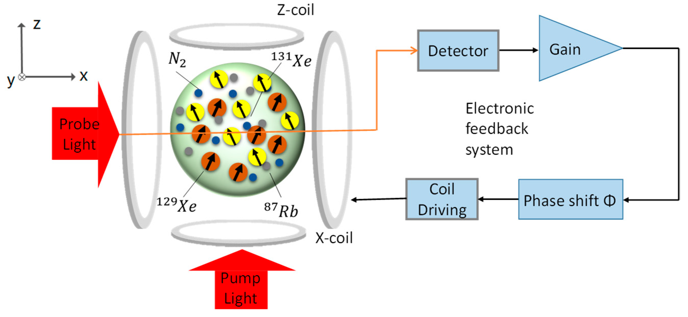
An NMRG using 129Xe and 131Xe is, in fact, a dual-species spin oscillator, as is shown in Figure 1 [1,11,14,15]. A vapor cell contains a mixture of gases, including 129Xe/131Xe, N2 and so on. To obtain angular momentum from the pump light, an excess amount of 87Rb is filled into the vapor cell. When heated, the 87Rb will vaporize and absorb pump light. The pump light is circularly polarized, so each photon carries angular momentum equal to one in the propagating direction. After taking in the circularly polarized photons, the spin of the 87Rb atom will align along the z-direction, i.e., become polarized. Through spin-exchange collisions, the angular momentum transfers from the 87Rb spins to the 129Xe/131Xe nuclear spins. As a result, the 129Xe/131Xe nuclear spins become polarized and give rise to a magnetization . A linearly polarized probe light transmits through the cell and interacts with the polarized 87Rb atoms. The polarization plane of the transmission light varies with the magnetic field sensed by the 87Rb atoms. Therefore, the magnetization of the nuclear spins can be detected. The output of the detector is sent to a signal processing system, which is used to obtain the magnetic field in the x and y directions. The y-axis magnetization component is amplified in the gain module, shifted by a phase of Φ, and then applied to drive the X-coil. For an appropriate gain and phase shift, the nuclear spins will precess continuously. More details for the NMRG can be found in [1].
The spin oscillator shown in Figure 1 actually has two spin oscillators: a 129Xe oscillator and a 131Xe oscillator. The 129Xe and 131Xe spins show negligible interaction through direct spin interaction, but coupling through the driving coil can occur. The driving fields of 129Xe and 131Xe influence each other, but this is not our concern here. In the following derivation, we will take the 129Xe spin oscillator as an example to describe the operating principle.
The motion of the spins satisfies the following Bloch equation [10,12]:
where is the magnetization of the spins, is the gyromagnetic ratio, is the magnetic field and is the rotation rate of the gyroscope with respect to the inertial frame.
Equation (1) shows that the rotation has the same effect as a magnetic field . Thus, we will discuss cross-coupling effects using the following equation:
Taking the relaxation time into account, Equation (2) can be expanded into the motion equation for the components of the magnetization:
where , and are the three components of the magnetization , respectively; , and are the three components of the magnetic field, respectively; and are the longitudinal spin relaxation time and the transverse relaxation time, respectively.
Defining a complex vector , and, from Equation (3), we can obtain:
To achieve analytical expressions for the oscillation frequency and amplitude for the 129Xe spin oscillator, we posit the following hypothesis. A static magnetic field with magnitude is applied along the z-axis, and a field is applied along the x-axis to drive the spins. The feedback system has limited bandwidth so that the components with a frequency out of the range of are filtered out. Here, is the bandwidth of the filter. Through adjusting the phase shift and gain in the feedback loop, the spin magnetization precesses about the z-axis with frequency in a clockwise manner. Therefore, we can write the following expressions:
where and are the components in the x and y-axes at , respectively.
With a rotatingwave approximation, we can describe the driving magnetic field for 129Xe as follows:
Inserting Equations (5) and (6) into Equation (4), we have:
where and is the in the steady state.
2.2. Modeling of a Spin Oscillator with a Cross-Axis-Rotation-Equivalent Magnetic Field
The influence of the cross-axis-rotation can be modeled by a transverse magnetic field; we might as well call this the cross-axis-rotation-equivalent (CARE) magnetic field. Without loss of generality, the CARE magnetic field can be described as follows:
where , and are the amplitude, angular frequency and phase of the n-th component, respectively.
With the CARE magnetic field, the motion of the spin oscillator still satisfies Equation (4), where . We assume that the spins still precess around the z-axis but that the angular frequency of and changes from to because of the CARE magnetic field; thus, we obtain the following expressions for the solutions of Equation (4):
where and are variations of the transverse and longitudinal magnetization due to the CARE magnetic field.
Inserting Equations (8) and (9) into Equation (4), we have:
Substituting Equations (7) and (9) into Equation (10), we have:
and:
Since the response of to an alternating magnetic field with angular frequency larger than is small, we might as well neglect terms that contain in Equation (12). As a result, Equation (12) can be reduced to:
Using the approximation that varies very slowly with time, we obtain the following equation from Equation (13):
In a practical case, the CARE field is usually small, so we replace the oscillating frequency with in the last term of Equation (14) to avoid the difficulty in solving the oscillating frequency. The validity of the approximation can be proved in the following simulation.
Equation (14) gives the Bloch–Siegert shift formula for spin oscillators [16,17,18]. It is clear that when , and vice versa. Thus, the rotating field pushes the oscillation frequency farther away from . When and , Equation (14) can be written as:
This is just the case of a Bloch–Siegert shift for only one linear driving magnetic field. When and , Equation (14) can be written as:
This is just the case of a cross-axis sensitivity effect when there is a static magnetic field in the xy-plane.
We can also obtain an approximate solution for from Equation (13) for only one CARE component, :
where .
When , Equation (17) becomes:
This means that if the CARE magnetic field has the same frequency as , the amplitude of the spin oscillator decreases. However, when is less than a specific value, the spin oscillator will be locked to the CARE field [19]. As a result, Equation (18) will not be valid. This can be seen in the following derivation. We assume there is only one component with frequency near , so we neglect other components. The CARE magnetic field can be described as:
and the feedback magnetic field can be described as:
where is a time varying phase.
We use the following expressions for the solutions of the Bloch equation:
Inserting Equations (19)–(21) into Equation (4), we have:
Substituting Equation (7) into Equation (22), we have:
and:
We make the approximation that and obtain from Equation (23):
Using the approximation that varies slowly with time, we obtain the following equation:
Neglecting the terms containing , Equation (26) can be reduced to:
This equation can be expressed as:
where , and are functions of , , , and . Equation (28) indicates that the spin oscillator can be locked to the CARE magnetic field when . This phenomenon is similar to the lock-in in ring laser gyroscopes [20,21]. A comprehensive analysis can be seen in [19].
We can obtain the lock-in threshold from Equation (27):
3. Numerical Simulation and Discussion
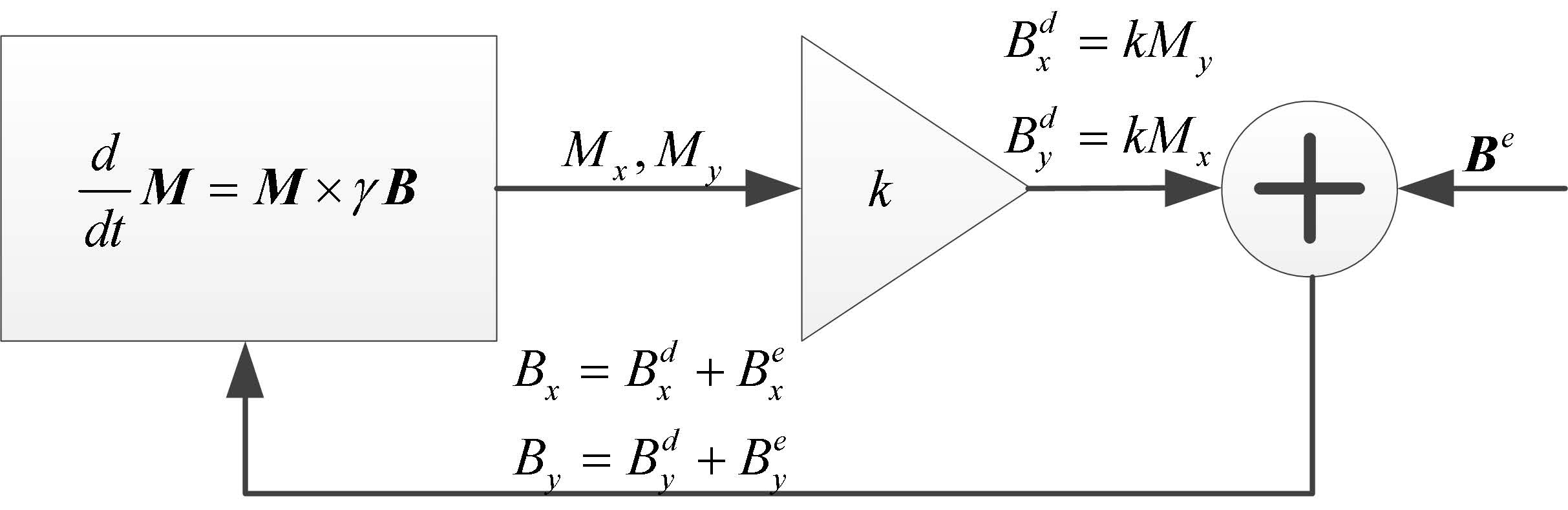
We carry out numerical simulation according to Equation (3). The simulation model based on Figure 1 is shown in Figure 2. The feedback magnetic field is and the CARE magnetic field is , . The parameters are as follows: = 30 s, = 20 s, = 1.5 μT, × 10 Hz/μT, = 100 A/m, = 0.0015. The initial values for the magnetization components are , and , respectively. Other parameters will be given in the specific simulation.
The Bloch equations were solved using the MATLAB ODE45 solver. The time step was 50 μs, and the time span was 0–1000 s. When we obtain the magnetization , we use the with a time span of 400 s–1000 s to make a fast Fourier transformation (FFT). We obtain the amplitude and frequency of the spin oscillator according to the peak in the FFT. With a timespan of 600 s, the frequency resolution is 0.0017 Hz and the obtained amplitude also shows errors due to limited data.
3.1. Frequency Shift due to a DC Magnetic Field
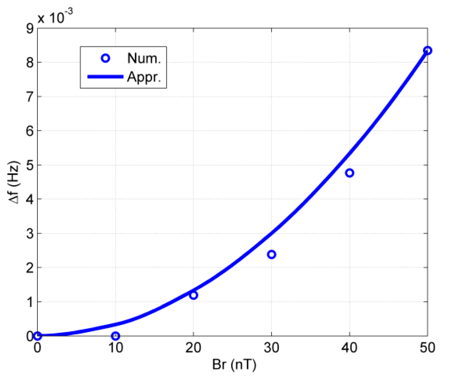
In this case, the CARE magnetic field is . In theory, the approximate analytical expression for the oscillation frequency shift will be . The simulation and approximate results are shown in Figure 3. It is clear that the approximate analytical results agree well with the numerical simulation results.
According to we know that the rotation for the y-axis will lead to an equivalent magnetic field. When the NMRG is placed in a vehicle, the maximum value of Ωy can be as high as 2π rad/s, equivalent to a magnetic field of 78 nT for the 129Xe spin oscillator and 284 nT for the 131Xe spin oscillator. When = 12 μT, the frequency shifts for 129Xe and 131Xe are 3.5 mHz and 11.8 mHz, respectively. This is a huge error for the NMRG, since it should measure Ωz with an error of less than 10 nHz for typical applications. To suppress this cross-axis effect, some methods can be used. For example, with a three-dimensional magnetic field compensation [22], the influence of low frequency Ωy can be suppressed greatly, but the bandwidth of the feedback loop should be as high as possible.
3.2. Frequency Shift due to an Oscillating Magnetic Field
3.2.1. One Component
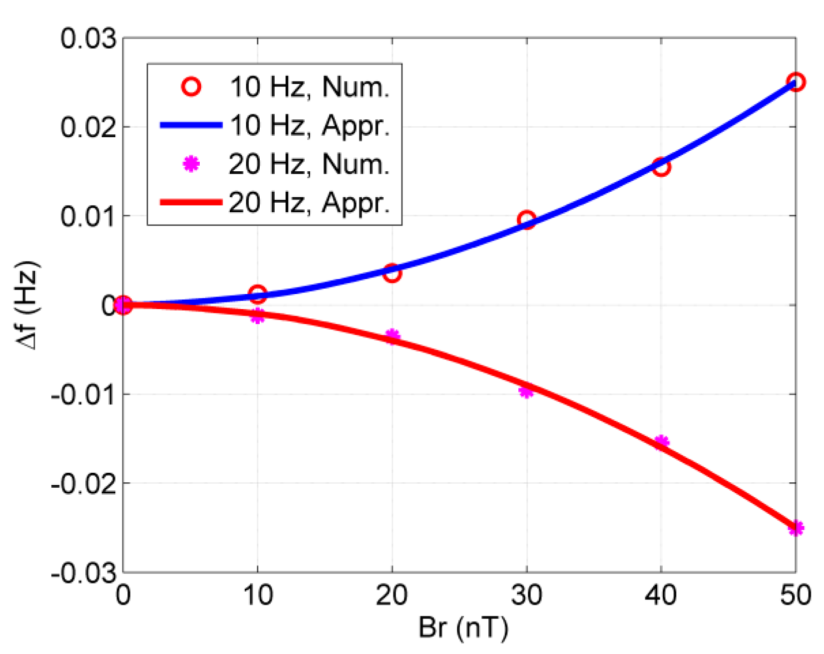
At first, we carry out simulations for the CARE magnetic field with only one frequency, where . According to a previous analysis, the approximate frequency shift will be . We choose two values and make the curve a function of . The simulation and approximate results are shown in Figure 4. The approximate analytical results agree well with the numerical simulation results.
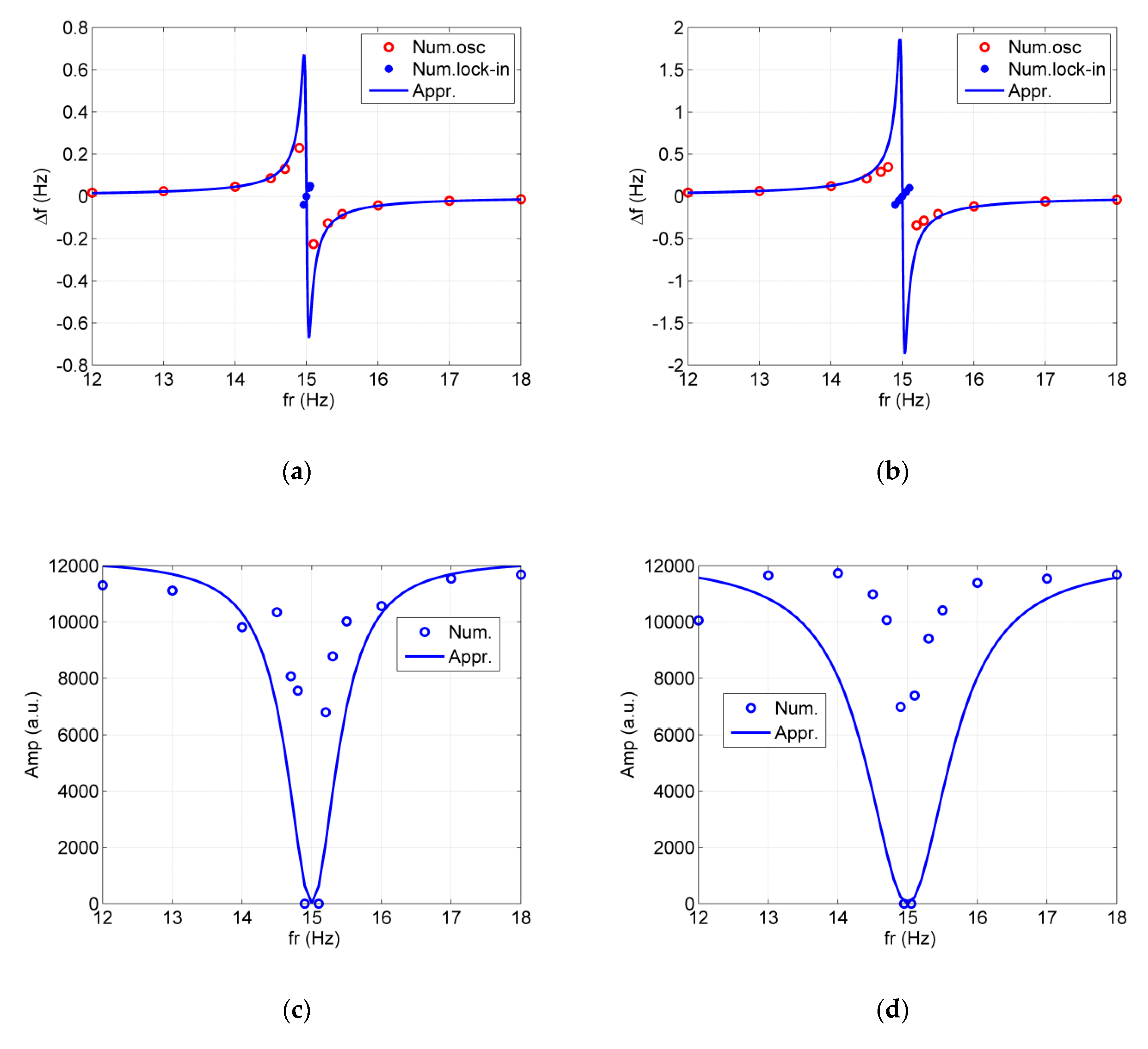
Next, at a specific magnetic field , we change the frequency . The frequency shift and amplitude of the spin oscillator are given in Figure 5. Here, denotes the amplitude of the spin oscillator without a CARE field. When , becomes very large. The relaxation time removes the frequency shift singular point when . At a specific , the spin oscillator is locked to the CARE magnetic field and its frequency is equal to . We also find that when approaches , the approximation solution has a larger error. The reason for this is that when approaches , we omitted some terms containing in the derivation for Equations (11) and (13). The approximation for Amp has a slightly larger error, but it still agrees with the numerical simulation qualitatively. That is, the CARE magnetic field near the Larmor frequency reduces the amplitude of the spin oscillator. It should be noted that the simulation program from Equation (3) also contributes to some error, which leads to the numerical data dispersion shown in Figure 5c,d.
3.2.2. Two Harmonic Components
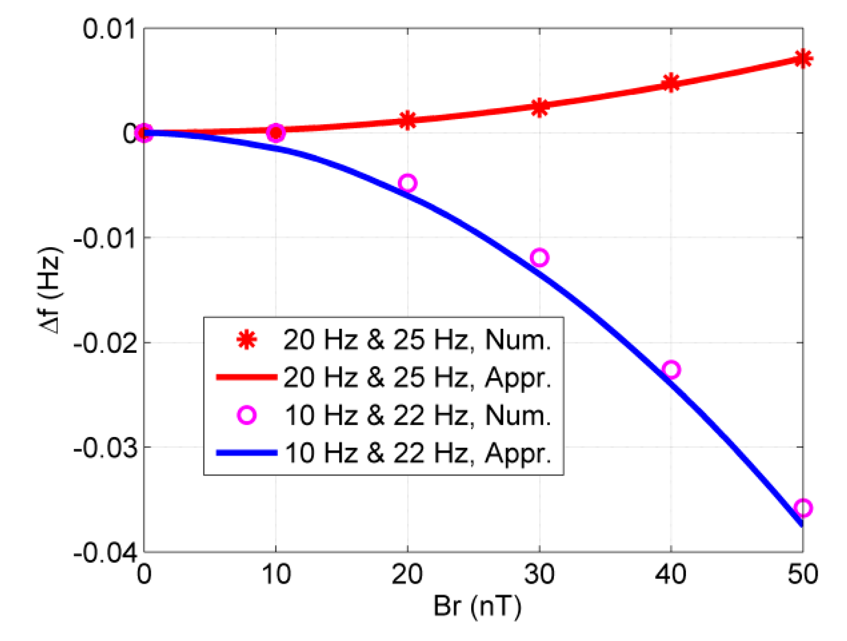
To check the approximate frequency shift in Equation (14) when the CARE magnetic field has more frequency components, we choose and to carry out numerical simulations. The approximate frequency shift is . Here, we choose . The results are shown in Figure 6, which shows that the approximate frequency shift agrees well with the numerical simulation.
3.3. Discussions
3.3.1. Comparing the 3He Gyroscope with a Dual-isotope Xe NMRG
Both the amplitude and frequency of the spin oscillator are changed due to the CARE magnetic field. The dynamical equation for analyzing the 3He gyroscope omitted the relaxation times T1 and T2 in Equation (3) and did not need the driving magnetic field. Therefore, the two types of gyroscopes are expected to show different behavior.
For a CARE magnetic field with very low frequency, the frequency shift for the two gyroscopes can be described by Equation (16). However, when the frequency of the CARE magnetic field is near the Larmor frequency, the 3He gyroscope loses signal periodically, and the amplitude of the Xe NMRG signal decreases. For the oscillation frequency of the Xe spin oscillator, it is locked to the frequency of the CARE magnetic field, and, out of the lock-in range, the oscillation frequency shifts according to Equation (14). This shows the CARE magnetic field pushes the oscillation frequency of a spin oscillator far away from the CARE magnetic field frequency. Therefore, the CARE magnetic field cannot be common-mode suppressed effectively by a dual-isotope scheme.
3.3.2. Methods to Reduce the Cross-Axis Effect
If the CARE magnetic field results from the rotation of a vehicle, it has a low frequency. Therefore, it is clear that we can reduce the cross-axis effect by increasing . Assuming a cross-axis input rotation rate of 1 rad/s, should be larger than 0.049 T for a 3He gyroscope [10]. This is not practical, since the magnetic inhomogeneity can be very large at this magnetic field. Fortunately, the transverse magnetic field in Xe NMRGs can be compensated by an alkali atom magnetometer and a feedback loop [22]. In general, a compensation bandwidth of approximately 10 Hz can be obtained.
For a high-frequency CARE magnetic field, the compensation loop cannot follow it in a timely manner. If the frequency spectrum of the angular vibration covers the Larmor frequency of the spin oscillator, it will cause a severe error. We might as well take the rotation component around the y-axis as an example to discuss the influence of the angular vibration [23,24]. We assume the rotation component has an amplitude of 0.003 rad/s at 100 Hz, corresponding to nT for 129Xe and nT for 131Xe. When μT, the frequency shifts of 129Xe and 131Xe due to the CARE magnetic field are 12.8 μHz and −3.7 μHz, respectively. Moreover, the worst case is a lock-in phenomenon, which makes the NMRG unresponsive toward . With s, rad/s and the lock-in threshold is approximately 0.17 °/s. It is a severe error for an NMRG.
To improve the tolerance of the NMRG toward the cross-axis angular vibration, it is better to choose a stronger , to ensure that the Larmor frequency is far away from the angular vibration component. The system level vibration isolation can also be used to attenuate possible angular vibration. In order to solve the lock-in problem, we can also use the biasing method just as that in ring laser gyroscopes, but it will make the NMRG more complicated.
4. Conclusions
In summary, we analyzed the response of a spin oscillator to a magnetic field in the xy-plane with both analytical and numerical methods. Approximate analytical equations for the frequency shift and amplitude of the spin oscillator with the CARE field are obtained, which are verified by solving the Bloch equations numerically. Then, we discussed the measurement error in an NMRG due to a rotation component in the x or y-axis. The NMRG is a single-axis gyroscope, but it also has cross-axis sensitivity to the x and y-axis. If the NMRG is subject to cross-axis rotation with a frequency near to its magnetic resonance frequency, the measurement error is relatively large, and the rotation rate cannot be measured. To reduce the cross-axis coupling effect, the resonance magnetic field should be as large as possible and a mechanical notch filter covering the oscillating frequencies of 129Xe and 131Xe can be used. These problems should be considered in the design of NMRG-based strap-down inertial navigation systems.
Author Contributions
Conceptualization, Z.W. and H.L.; methodology, Z.W.; software, Z.W.; validation, Y.Z., X.Z. and Q.J.; writing—original draft preparation, Z.W.; writing—review and editing, Z.W., Y.Z., X.Z. and Q.J.; project administration, Z.W. and H.L.; funding acquisition, Z.W. and H.L. All authors have read and agreed to the published version of the manuscript.
Funding
This research was funded by the National Natural Science Foundation of China (Grant No. 61671458, 61701515), the Natural Science Foundation of Hunan (Grant No. 2018JJ3608) and the Research Project of the National University of Defense Technology (Grant No. ZK170204), China Postdoctoral Science Foundation (Grant No. 2017M613367).
Conflicts of Interest
The authors declare no conflicts of interest.
References
- Eklund, E.J. Microgyroscope Based on Spin-Polarized Nuclei. Ph.D. Thesis, University of California, Irvine, CA, USA, 2008. [Google Scholar]
- Walker, T.G.; Larsen, M.S. Spin-Exchange Pumped NMR Gyros. Adv. Atom. Mol. Opt. Phy. 2016, 65, 373–401. [Google Scholar]
- Larsen, M.; Bulatowicz, M. Nuclear magnetic resonance gyroscope. IEEE Freq. Control Symp. 2012, 978, 1–5. [Google Scholar]
- Donley, E. Nuclear magnetic resonance gyroscopes. In Proceedings of the SENSORS, 2010 IEEE, Kona, HI, USA, 1–4 November 2010. [Google Scholar]
- Meyer, D.; Larsen, M. Nuclear magnetic resonance gyro for inertial navigation. Gyroscopy Navig. 2014, 5, 75–82. [Google Scholar] [CrossRef]
- Woodman, K.F.; Franks, P.W.; Richards, M.D. The nuclear magnetic resonance gyroscope: A review. J. Navig. 1987, 40, 366–384. [Google Scholar] [CrossRef]
- Fang, J.C.; Qin, J. Advances in atomic gyroscopes: A view from inertial navigation applications. Sensors 2012, 12, 6331–6346. [Google Scholar] [CrossRef] [PubMed]
- Qin, J.; Wang, S.; Gao, P.; Wang, Y.; Han, W. Advances in nuclear magnetic resonance gyroscope. Navig. Positioning Timing 2014, 1, 64–69. [Google Scholar]
- Shaw, G.L. Sensitivity to cross-axis oscillations in a single-axis nuclear gyroscope. J. Guid. Control Dynam. 1984, 7, 501–502. [Google Scholar] [CrossRef]
- Shaw, G.L. 3He Nuclear Gyroscope. Available online: https://apps.dtic.mil/dtic/tr/fulltext/u2/a159924.pdf (accessed on 29 January 2020).
- Wang, Z.G.; Peng, X.; Luo, H.; Guo, H. Comparison of operation modes for spin-exchange optically-pumped spin oscillators. J. Magn. Reson. 2017, 278, 134–140. [Google Scholar] [CrossRef] [PubMed]
- Abragam, A. The Principles of Nuclear Magnetism; Oxford University Press: London, UK, 1961. [Google Scholar]
- Guerinoni, L.; Falorni, G.L.; Gattere, G. Modelling Cross Axis Sensitivity in MEMS Coriolis Vibratory Gyroscopes. Proceedings 2017, 1, 281. [Google Scholar] [CrossRef] [Green Version]
- Bulatowicz, M.; Griffith, R.; Larsen, M.; Mirijanian, J.; Fu, C.B.; Smith, E.; Snow, W.M.; Yan, H.; Walker, T.G. Laboratory search for a long-range T-Odd, P-Odd interaction from axionlike particles using dual-species nuclear magnetic resonance with polarized 129Xe and 131Xe gas. Phys. Rev. Lett. 2013, 111, 102001. [Google Scholar] [CrossRef] [PubMed] [Green Version]
- Yoshimi, A.; Asahi, K.; Sakai, K.; Tsuda, M.; Yogo, K.; Ogawa, H.; Suzuki, T.; Nagakura, M. Nuclear spin maser with an artificial feedback mechanism. Phys. Lett. A 2002, 304, 13–20. [Google Scholar] [CrossRef]
- Pendlebury, J.M.; Heil, W.; Sobolev, Y.; Harris, P.G.; Richardson, J.D.; Baskin, R.J.; Doyle, D.D.; Geltenbort, P.; Green, K.; van der Grinten, M.G.D.; et al. Geometric-phase-induced false electric dipole moment signals for particles in traps. Phy. Rev. A 2008, 70, 32102. [Google Scholar] [CrossRef] [Green Version]
- Bloch, F.; Siegert, A. Magnetic resonance for nonrotating fields. Phy. Rev. 1940, 57, 522–527. [Google Scholar] [CrossRef]
- Ramsey, N.F. Resonance transitions induced by perturbations at two or more different frequencies. Phys. Rev. 1955, 100, 1191–1194. [Google Scholar]
- Pavlov, Y.V.; Pivkin, A.N.; Umarkhodzhaev, R.M.; Lariontsev, E.G. Synchronization with harmonics in an injected nuclear-magnetic-resonance laser. Phy. Rev. A 2010, 82, 33802. [Google Scholar] [CrossRef]
- Chow, W.W.; Gea-Banacloche, J.; Pedrotti, L.M.; Sanders, V.E.; Schleich, W.; Scully, M.O. The ring laser gyro. Rev. Mod. Phys. 1985, 57, 61–103. [Google Scholar] [CrossRef]
- Krobka, N.I.; Türkin, D.A. Laser gyros frequency biasing and fiber optic gyros phase biasing: Similarities and differences. In Proceedings of the 2017 24th Saint Petersburg International Conference on Integrated Navigation Systems (ICINS), St. Petersburg, Russia, 29–31 May 2017. [Google Scholar]
- Grover, B.C.; Kanegsberg, E.; Mark, J.G.; Meyer, R.L. Nuclear Magnetic Resonance Gyro. U.S. Patent 4,157,495, 5 June 1979. [Google Scholar]
- Lee, J.P.; Whaley, W. Prediction of the angular vibration of aircraft structures. J. Sound Vib. 1976, 49, 541–549. [Google Scholar] [CrossRef]
- Merritt, P.; Donaldson, J.; O’Brien, D.; Coleman, K.; Pyles, G. Angular vibration survey of various aircraft. In Proceedings of the Laser Systems Technology, Orlando, FL, USA, 21–25 April 2003. [Google Scholar]
Figure 1.
Principle of a dual-species spin oscillator.

Figure 2.
Simulation model corresponding to the NMRG principle given in Figure 1.
Figure 2.
Simulation model corresponding to the NMRG principle given in Figure 1.

Figure 3.
The frequency shift vs. DC magnetic field in the y-axis. “Num.” and “Appr.” in the figure denote numerical and approximate analytical results, respectively.
Figure 3.
The frequency shift vs. DC magnetic field in the y-axis. “Num.” and “Appr.” in the figure denote numerical and approximate analytical results, respectively.

Figure 4.
The frequency shift vs. Br for different frequencies of the Cross-Axis-Rotation-Equivalent (CARE) magnetic field.
Figure 4.
The frequency shift vs. Br for different frequencies of the Cross-Axis-Rotation-Equivalent (CARE) magnetic field.

Figure 5.
The frequency shift and amplitude Amp of the spin oscillator vs. frequencies of the CARE magnetic field. (a) vs. for = 30 nT; (b) vs. for = 50 nT; (c) Amp vs. for = 30 nT; (d) Amp vs. for = 50 nT. In (a,b), Num. lock-in denotes the frequency shift in the lock-in state. In the lock-in state of (c,d), we let Amp = 0 to express that the spin oscillator cannot normally measure the rotation rates. In fact, the amplitude and frequency of the spin oscillator in the lock-in state is governed by the CARE magnetic field. The limited data for FFT contribute to the scattering of frequency shift and Amp to some extent.

Figure 6.
The frequency shift vs. magnetic field amplitude for different groups of magnetic fields. Two groups of magnetic field are given: one is Hz and Hz while another is 10 Hz and Hz.
Figure 6.
The frequency shift vs. magnetic field amplitude for different groups of magnetic fields. Two groups of magnetic field are given: one is Hz and Hz while another is 10 Hz and Hz.

© 2020 by the authors. Licensee MDPI, Basel, Switzerland. This article is an open access article distributed under the terms and conditions of the Creative Commons Attribution (CC BY) license (http://creativecommons.org/licenses/by/4.0/).
Share and Cite
MDPI and ACS Style
Wang, Z.; Zhang, Y.; Zhan, X.; Jiang, Q.; Luo, H. Cross-Axis Coupling Effects in Single-Axis Nuclear Magnetic Resonance Gyroscopes. Sensors 2020, 20, 734. https://doi.org/10.3390/s20030734
AMA Style
Wang Z, Zhang Y, Zhan X, Jiang Q, Luo H. Cross-Axis Coupling Effects in Single-Axis Nuclear Magnetic Resonance Gyroscopes. Sensors. 2020; 20(3):734. https://doi.org/10.3390/s20030734
Chicago/Turabian StyleWang, Zhiguo, Yi Zhang, Xiang Zhan, Qiyuan Jiang, and Hui Luo. 2020. "Cross-Axis Coupling Effects in Single-Axis Nuclear Magnetic Resonance Gyroscopes" Sensors 20, no. 3: 734. https://doi.org/10.3390/s20030734
Note that from the first issue of 2016, this journal uses article numbers instead of page numbers. See further details here.