Photovoltaic Array Fault Diagnosis Based on Gaussian Kernel Fuzzy C-Means Clustering Algorithm


School of Automation, Beijing Institute of Technology, Beijing 100081, China
*
Author to whom correspondence should be addressed.
Sensors 2019, 19(7), 1520; https://doi.org/10.3390/s19071520
Submission received: 23 February 2019
/
Revised: 20 March 2019
/
Accepted: 23 March 2019
/
Published: 28 March 2019
(This article belongs to the Section Physical Sensors)
Abstract
:In the fault diagnosis process of a photovoltaic (PV) array, it is difficult to discriminate single faults and compound faults with similar signatures. Furthermore, the data collected in the actual field experiment also contains strong noise, which leads to the decline of diagnostic accuracy. In order to solve these problems, a new eigenvector composed of the normalized PV voltage, the normalized PV current and the fill factor is constructed and proposed to characterize the common faults, such as open circuit, short circuit and compound faults in the PV array. The combination of these three feature characteristics can reduce the interference of external meteorological conditions in the fault identification. In order to obtain the new eigenvectors, a multi-sensory system for fault diagnosis in a PV array, combined with a data-mining solution for the classification of the operational state of the PV array, is needed. The selected sensors are temperature sensors, irradiance sensors, voltage sensors and current sensors. Taking account of the complexity of the fault data in the PV array, the Kernel Fuzzy C-means clustering method is adopted to identify these fault types. Gaussian Kernel Fuzzy C-means clustering method (GKFCM) shows good clustering performance for classifying the complex datasets, thus the classification accuracy can be effectively improved in the recognition process. This algorithm is divided into the training and testing phases. In the training phase, the feature vectors of 8 different fault types are clustered to obtain the training core points. According to the minimum Euclidean Distances between the training core points and new fault data, the new fault datasets can be identified into the corresponding classes in the fault classification stage. This strategy can not only diagnose single faults, but also identify compound fault conditions. Finally, the simulation and field experiment demonstrated that the algorithm can effectively diagnose the 8 common faults in photovoltaic arrays.
1. Introduction
With the intensification of the energy and environment crisis, clean energy plays an integral role in restraining global warming issues and has received more and more attention in industrial circles. As a major clean energy technology, photovoltaic power generation has received worldwide attention in recent years, especially in developing countries. Online intelligent multisensor monitoring systems are the guarantee of stable operation for the PV system. This direction is increasingly becoming a research hotspot in academic circles. Once the signal from the sensors have been acquired, various diagnostic techniques of the PV array can be adopted to extract as much information as possible from these signals. Furthermore, suitable decision-making strategies can be built up for failure detection of a PV array. A variety of studies have applied different diagnostic approaches to conduct this industrial task. In paper [1,2], Takashima T et al. used the acquired voltage and current signals to propose time domain reflectometry (TDR) and earth capacitance measurement (ECM) to detect the positions of the open circuit points in the circuits. Hu Y et al. presented a Thermography-based temperature distribution analysis method to identify PV module mismatch faults [3]. Nuri Gokmen et al. only measured the operating voltage of PV string and ambient temperature to efficiently detect the number of open and short circuit faults and discriminate between them and partial shading conditions [4]. Siva Ramakrishna Madeti, S.N. Singh proposed a program that using minimum number of voltage sensors to locate fault modules. The main advantage of this algorithm is that it voids the need of current sensors and reduces the number of the sensors used [5]. A. Chouder and S. Slivestre defined two new power loss indicators, including thermal capture losses and miscellaneous capture losses, to classify different fault types in PV system operations [6]. The line-to-line (LLF), ground fault (GF) and arc fault (AF) are generally considered to be the main catastrophic failures in a PV array [7,8,9]. Arc faults cause continuous oscillations and distortions in the output current and voltage waveforms of the inverter. Then the diagnosis of the fault type replies on a suitable time-frequency domain analysis on the voltage and current waveforms [10,11,12]. Fault detection in a PV array becomes difficult under low irradiance conditions. Line-to-line faults and ground faults may be undetected in the low irradiance situation. Artificial intelligence (AI) techniques are considered to be promising strategies to address with these problems. Zhehan Yi and Amir H. Etemadi proposed a multi-resolution signal decomposition method to extract fault features and two intelligent classification methods to identify the line-to-line and ground faults [13,14]. In addition, there are some other AI techniques for detecting the faults in a PV array. The strategy based on the fault threshold and Back Propagation (BP) neural networks was proposed in the paper [15] to detect 8 fault types at three levels including component, branch and array. In the literature [16], a multi-class support vector machine was designed to diagnose the line-to-line faults and the aging faults in the photovoltaic array. Zhao Y et al. [17] developed a graph-based semi-supervised detection method for discriminating different faults including short circuits, open circuits and line-to-line faults, and so on. The paper [18] proposed a density peak-based clustering approach for fault diagnosis in PV arrays. However, this approach needs the predetermination of the clustering number. Bi Rui et al. [19] combined the open circuit voltage Voc, short circuit current Isc, maximum power voltage Vmpp and maximum power current Impp as the feature vectors to characterize different fault types, then the Fuzzy C-means clustering method (FCM) was used to classify these faults.
Under the operating conditions, some single faults and compound faults display similar features and the fault datasets acquired in the field experiment are usually accompanied by environmental and system noise. These two points lead to the fault classification difficulty that some single faults and compound faults with similar characteristics cannot be discriminated by the conventional feature quantities proposed in previous papers. The conventional feature quantities mainly contain voltage, current, power, Vnorm, Inorm, FF (Vnorm, Inorm), and so on. In order to realize a good degree of fault discrimination, a new eigenvector composing of Vnorm, Inorm and FF was constructed to characterize 8 different faults in three-dimension space. The simulation results show that the proposed feature vectors can separate these faults effectively in noise-free conditions. As a result of the noise existing in the data collecting process of the field experiment, the new feature vectors cannot distinguish the 8 faults in the operating condition obviously. The Gaussian Kernel Fuzzy C-means clustering method (GKFCM) is an unsupervised learning clustering algorithm that using kernel function to map the sample data in the original space to a high-dimension space and then adopting the similarity function to classify the fault datasets. Compared to the traditional fuzzy C-means clustering algorithm, the GKFCM can highlight the difference of the sample characteristics by the nonlinear mapping of kernel space. This method can improve the clustering ability of complex datasets and robustness of fault diagnosis effectively. Therefore, a new fault classification method based on the GKFCM with the new eigenvectors (Vnorm, Inorm, FF) is propounded in this paper. In the first phase of the algorithm, the different faults are characterized by the new eigenvectors and achieves a preliminary distinction. Then, the different fault datasets are input into the GKFCM to train and test for drawing fault diagnostic conclusions. Since the proposed method considers the normalization of the feature quantities and the robustness of the GKFCM, the generalization ability of the fault diagnostic algorithm can be further guaranteed.
2. Gaussian Kernel Fuzzy C-Means Clustering Method
The gaussian kernel fuzzy C-means clustering method contains two steps: firstly, the original space X is mapped to high-dimension space F by the Gaussian Kernel Function and then using the clustering algorithm to classify different datasets. The GKFCM can highlight the difference of the sample features by the non-linear mapping operation in the kernel space. This method is suitable for the classification problems with similar sample characteristics [20,21,22,23,24,25,26]. The nonlinear mapping function is defined as follow:
where is the sample of the original space X. The objective function of the clustering algorithm is given by
where is the core point of the original sample space; is the clustering number; is the sample number in the original sample space; is the membership between the sample and the fault class. satisfies three conditions including , and ; is a weighted parameter.
The kernel function is defined as follows:
Therefore, the Euclidean distance in Equation (2) is given by
The common kernel functions generally contain the Gaussian kernel function, polynomial kernel function and Sigmoid kernel function. The Gaussian kernel function is adopted in this paper and shown as the Equation (5).
where represents the parameter of Gaussian kernel function.
Altogether, the Equation (2) uses the constraints and the Lagrange multiplier approach to find and . The parameters and are shown as the Equations (6) and (7).
3. The Fault Diagnosis Algorithm Based on GKFCM
The fault diagnosis method based on the GKFCM is divided into two stages: the training and testing phases. In the training stage, using the training fault datasets to train the GKFCM and taking the fault classification error as the principle of the training performance. When the classification error reaches the minimum level, the core points are calculated and obtained. The classification error equation is shown by
where and are the class fault dataset and its corresponding sample number, respectively. is the sample number of the fault dataset. belongs to the fault class after the GKFCM clustering.
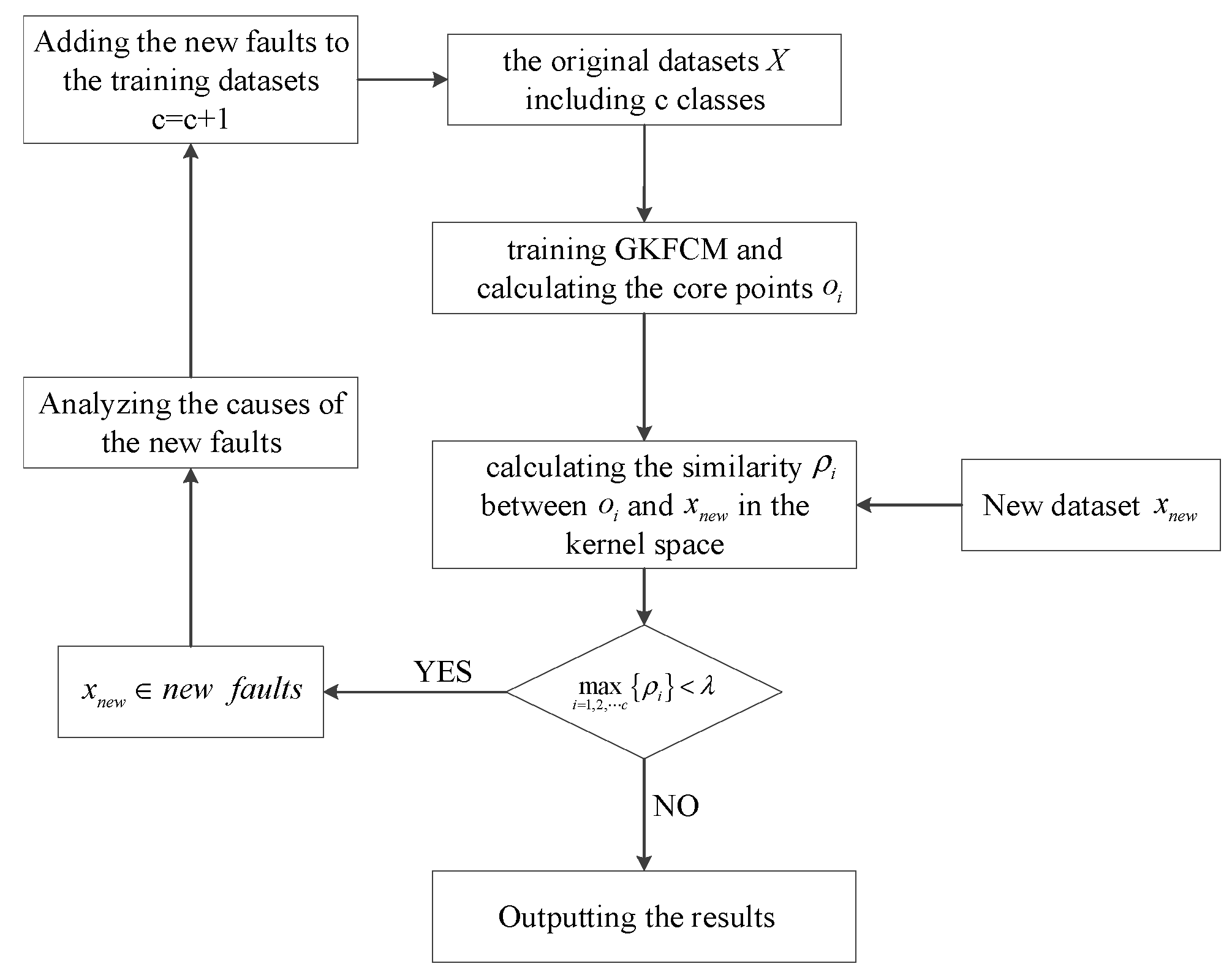
In the testing phase, the similarity between the new fault data and the center points of the reference fault datasets is used to judge the fault category of the new fault data. The steps of the fault diagnosis are listed as follows:
- Using the fault datasets including classes as the training datasets
- According to the Equation (7), the core points of the reference datasets are calculated and obtained when the classification error rate reaches the minimum level.
- Using the Equations (9) and (10) to determine the fault type of the new sample in the testing datasets.where is the similarity between and the dataset . The larger the value of , the higher the possibility of belonging to the corresponding fault type [15]. The Equation (8) is the judging criteria for the classification of the datasets in Support Vector Machine (SVM) and we use this principle to discriminate different fault datasets in this paper. is the category attribution threshold and the value is generally distributed between 0 and 0.5 [15,16].
- The previous step can not only determine the known faults in the training datasets but also judge the unknown fault types. If the belongs to an unknown fault, it will be classified as the class.
The flow chart of the proposed fault diagnostic method are described as Figure 1.
4. The Fault Diagnosis Method Based on GKFCM for the Photovoltaic Arrays
4.1. Selection of the Fault Feature Quantities
In order to obtain a good diagnostic accuracy, three characteristics are constructed and combined as the feature vector for characterizing different fault types of PV array [16,17,18,27].
- The normalized PV voltage Vnormwhere is the open circuit voltage of the reference PV module. is the module number in each branch.
- The normalized PV current Inormwhere is the short circuit current of the reference PV module. is the branch number of the PV array.
- The Fill Factor (FF)where is the open circuit voltage of the PV array and is the short circuit current of the PV array.
The PV array is designed as the research object in this paper and the detailed operating conditions contains four categories: normal, open circuit, short circuit and compound fault conditions. There are 8 fault types in total. is the number of the fault types and equals to 8. The 8 fault types of the photovoltaic array are simulated in the simulation and the fault feature vectors that characterizing the 8 faults are acquired and shown as the Equation (14).
where X is the datasets of 8 fault types. is the sample number of each fault.
4.2. Procedures of PV Array Fault Detection Approach Based on GKFCM
- Firstly, using the acquired datasets of 8 fault types to train the GKFCM. The core points are obtained when the classification error reaches the minimum level.
- Secondly, substituting the new fault dataset into the trained GKFCM and using the Equations (9) and (10) to judge the fault types of the new fault data .
- Lastly, judging the fault type based on the maximum similarity between the center points of the reference fault datasets and the new fault . If is not the known fault types included in the reference fault datasets, a new procedure is conducted to identify the fault type of . Then using it as a new fault type to train GKFCM to get a new training model.
5. The Simulation Experiment
5.1. Model of the Photovoltaic Array
The single diode model (SDM) shown as Equation (15) is the most commonly utilized model [28,29,30]. It is used to construct the PV array to mimic accurately solar cells and PV modules behaviors in this paper.
The parameters of the PV module in the simulation are listed in Table 1.
The simulation model of the PV array is shown in Figure 2.
The wide-weather environment conditions in simulation experiment are set as the ranges of solar irradiance varying from 100 to 1000 W/m2 with step of 50 W/m2 and the backplane temperature changing from 0 °C to 40 °C with step of 1 °C. The 8 fault types can be simulated and carried out by the different combinations of Air Switches (AS) shown in Figure 2. The detailed descriptions of 8 fault types are listed in Table 2.
In the simulation experiment, 779 samples were acquired in each fault type of the 8 faults and 6332 fault samples were obtained in total.
5.2. The Feature Characteristic Analysis of 8 Fault Types
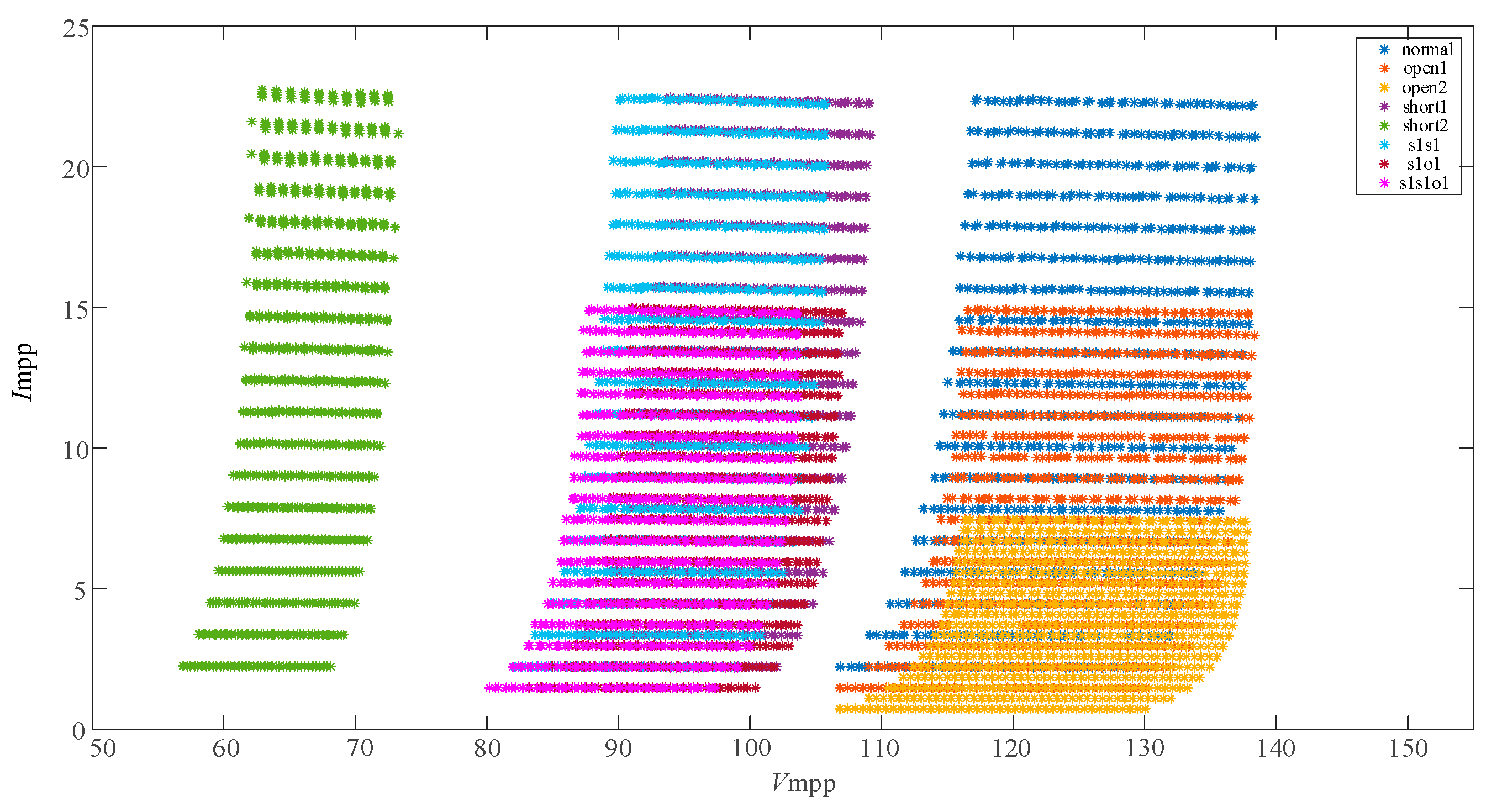
The conventional feature vectors were used to characterize the 8 fault types in the paper [6] and the distribution of the eigenvectors are shown in Figure 3. It is obvious that the 8 fault types overlap seriously and they are difficult to differentiate.
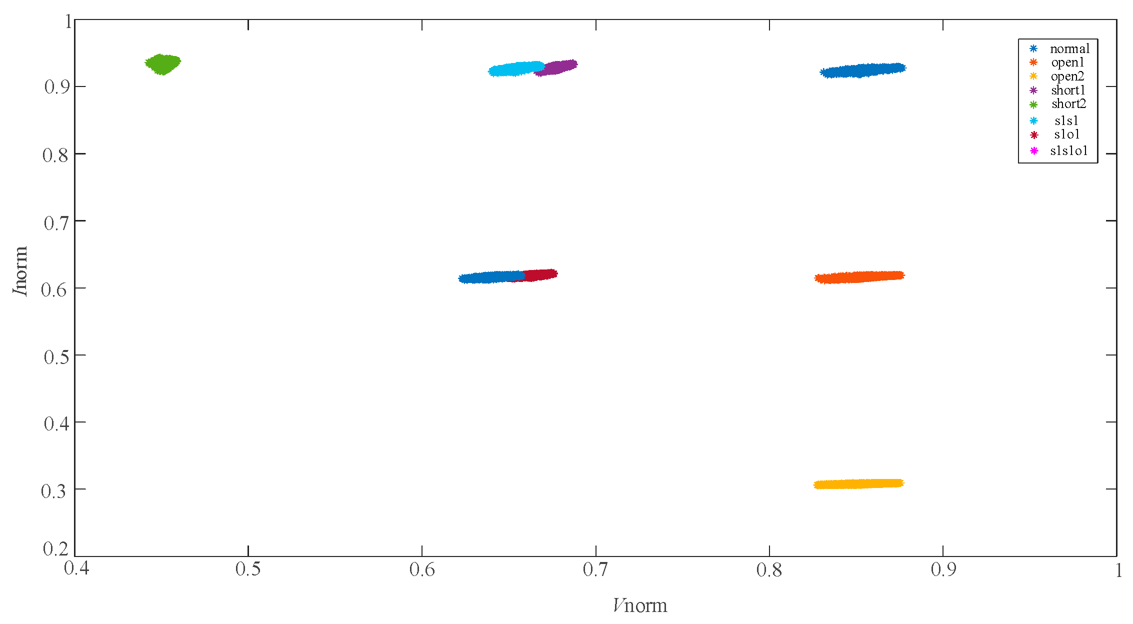
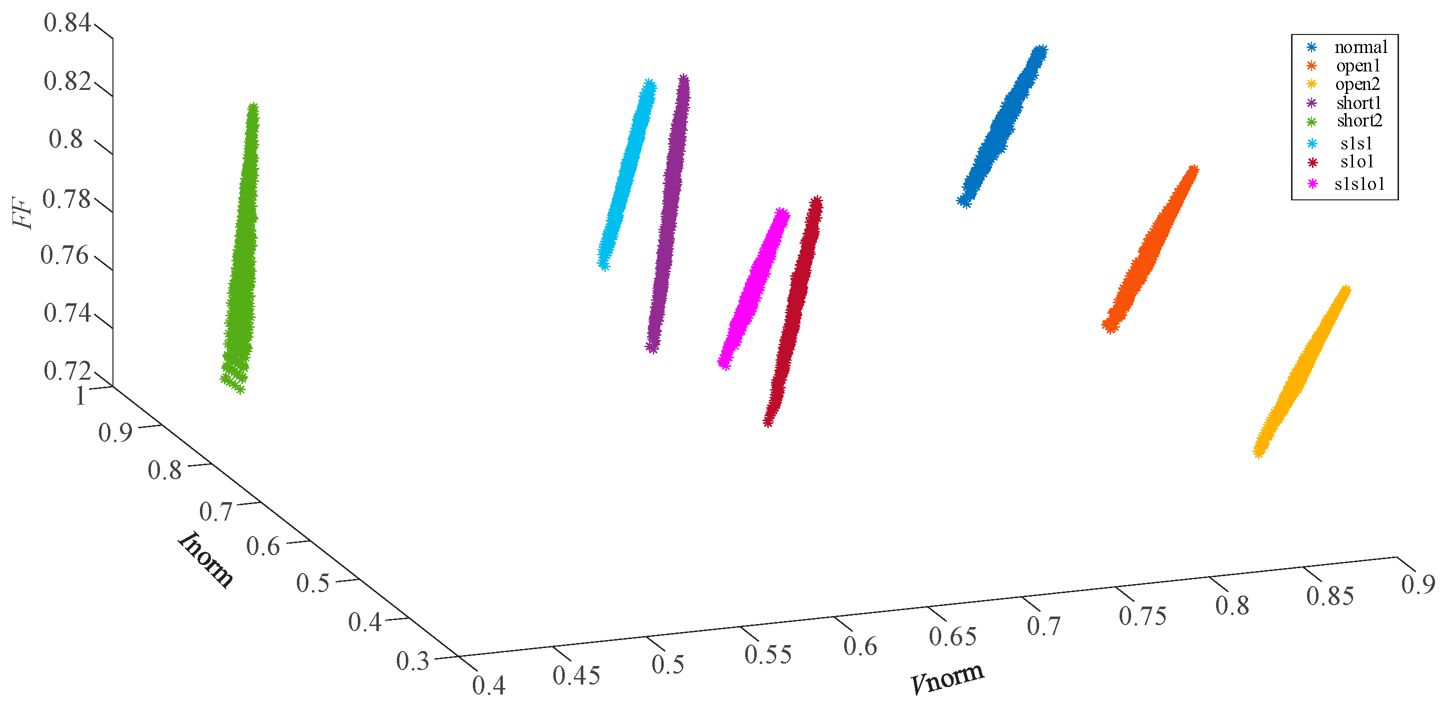
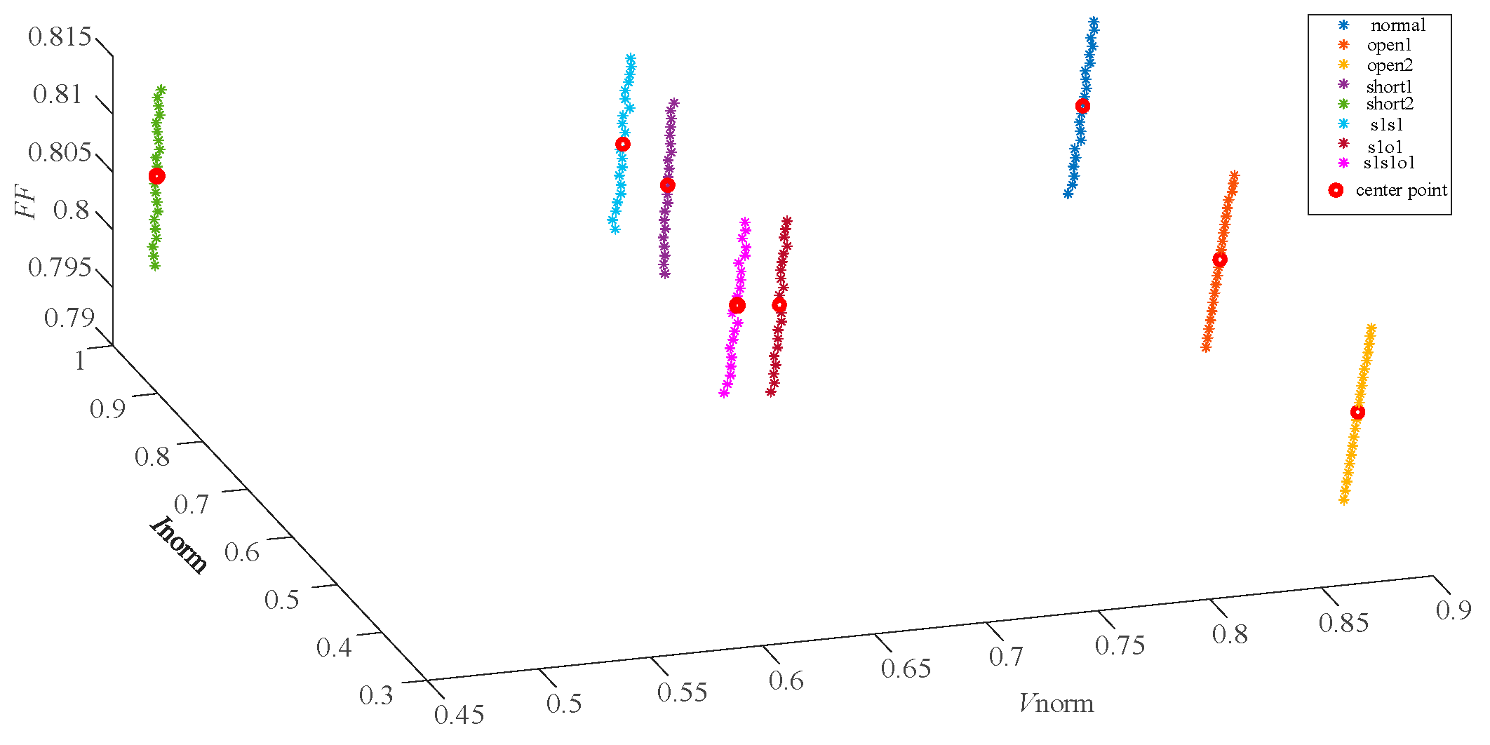
In the paper [6,7], the eigenvectors of 8 fault types are tranformed and improved as for further discriminating the overlapping faults. The distribution of the feature vectors are described in Figure 4 and the faults are mostly separated. However, short1 and s1s1, s1o1 and s1s1o1 still overlap with each other. The data distribution in Figure 3; Figure 4 indicates that the eigenvectors and have limitations in differentiating the single faults and compound faults with similar characteristics. It was found that the Filling Factor (FF) of each fault case was different through the in-depth research. So, the normalized PV voltage Vnorm, the normalized PV current Inorm and the Fill Factor (FF) were combined together as a new eigenvector to further characterize 8 different fault types. The results, showing use of the feature vectors for fault characterization of the 8 faults, are shown in Figure 5.
The distribution of the eigenvectors in Figure 5 demonstrates that the newly proposed feature vector can discriminate the 8 fault types obviously. This new eigenvector is appropriate for describing and characterizing some complex operating conditions, including single and compound faults with similar characteristics.
5.3. Simulation Results
Figure 5 gives an intuitive display that 8 faults can be separated by the eigenvectors . However, the actual data acquisition process is usually accompanied by the noise of the environment and acquisition devices. Therefore, the fault datasets acquired are complex and the differentiation degree of each fault is not obvious. Since GKFCM can effectively improve the clustering performance of the complex datasets, this clustering algorithm was adopted to cluster and identify fault types in this article. The classification and identification of the new fault datasets is based on the maximum similarity between the new fault datasets and the core points of the reference datasets. As the distribution of the 8 fault types is relatively concentrated in Figure 5, a small part of the fault datasets in wide-weather environmental conditions can be used as the reference datasets to train the GKFCM and then identify the new fault datasets. The environmental parameters in the 8 fault datasets collection process are listed in Table 3.
In the training phase of the simulation, the detailed parameters of GKFCM were set as follows: the clustering number was 8, weighted index was 2, the maximum number of the iterations was 1000 and the limitation of the iteration was the minimum similarity with the value 10−5.
The Figure 6 shows the distribution of the 8 faults in the simulated training datasets and the red points are the cores of each clustering. The center-point coordinates of the 8 clusterings in the reference fault datasets are listed in Table 4.
In the testing stage, each dataset of 8 fault types contained 110 samples. The Equations (9) and (10) were used to calculate the similarity of the new fault datasets and the core points in the reference fault datasets. is set as 0.5 and the results of the classification are listed in Table 5.
In summary, the overall diagnostic accuracy was 100%. The simulation experiment shows that the proposed method has a good fault diagnostic performance.
6. The Field Experiment
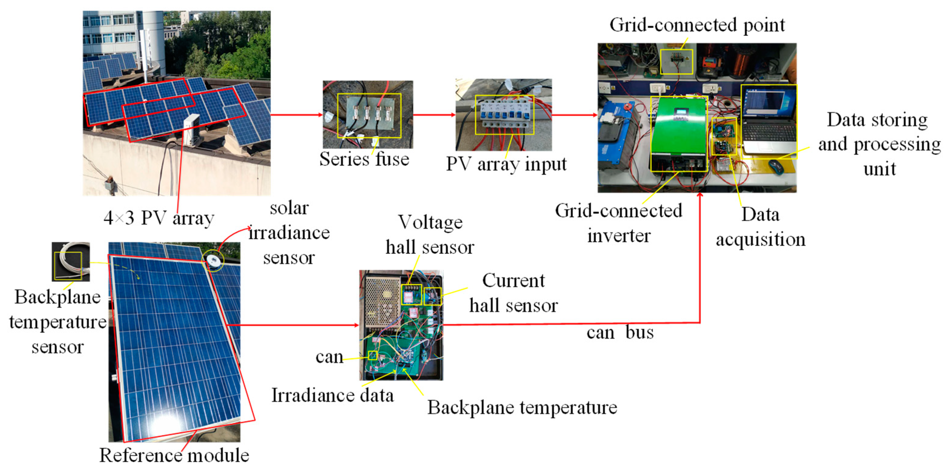
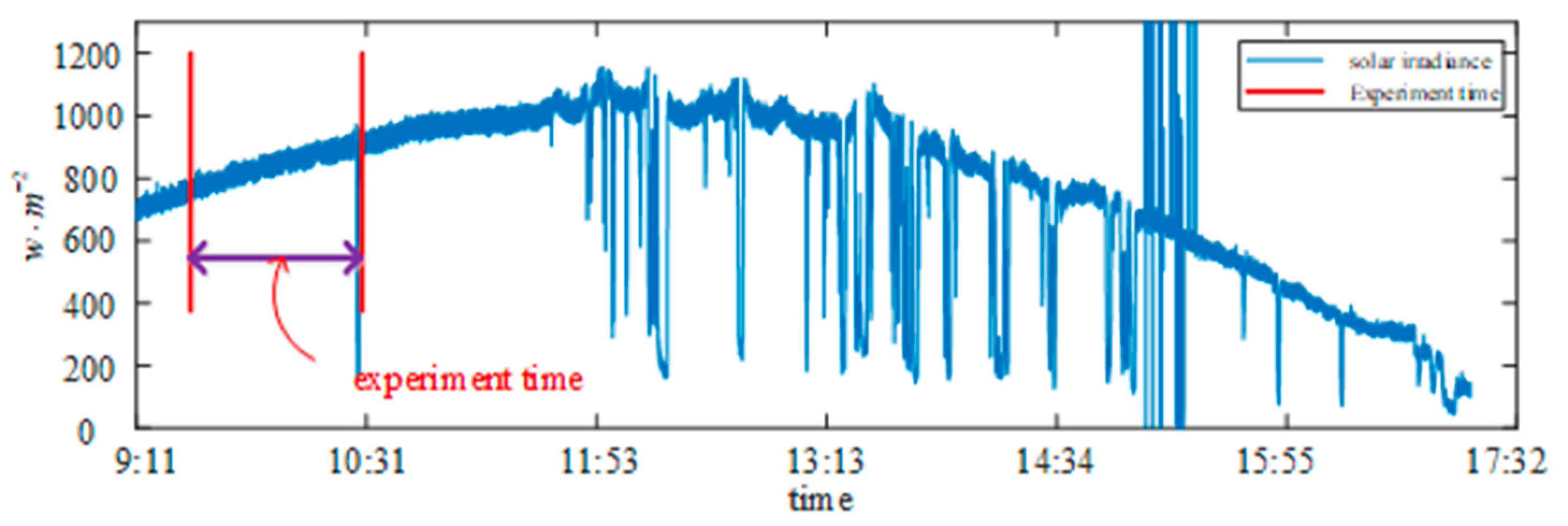
In the field experiment, the GSP-240 PV module was used to build the PV array for validating the proposed fault diagnostic method. The key specifications of GSP-240 module are listed in Table 6 and the experiment platform is shown in Figure 7. The field experiment platform contained PV array, 5 KW inverter, a series fuse, a combiner box and the data collecting and recording system. The data acquisition system consists of a temperature sensor, a solar irradiance sensor and two pairs of current and voltage sensors. The first two sensors and one pair of current and voltage sensors were located on the reference module. They were used to collect meteorological information, the short circuit current and open circuit voltage of the reference module, respectively. The operating voltage and current signals of PV array were measured by means of the other pair of the current and voltage sensors. This set of sensors shown in the data acquisition board in Figure 7 were mounted at the input of the converter. In total, a 6-sensor system was developed for online monitoring of the PV array. In this experiment, eight fault datasets were simulated by different combination of the air breakers and the different fault datasets were collected from 09:30 to 10:30 on 7 September 2018. In the fault datasets, each fault dataset owns 180 samples. Therein, 60 fault samples of each class were defined as the training datasets and the remaining 120 samples in each fault type were divided as the testing datasets.
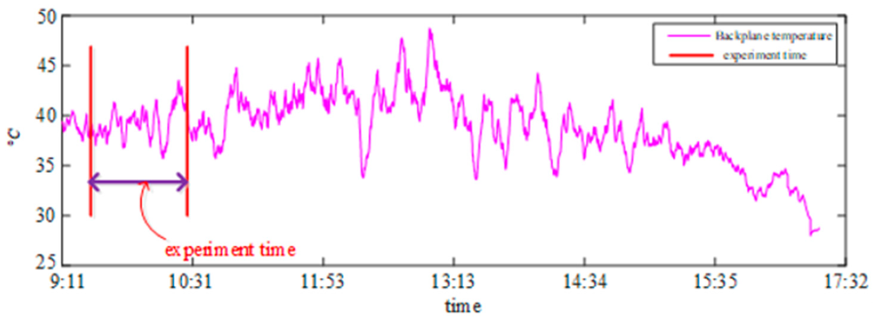
The range of the irradiance and backplane temperature in the daytime on 7 September 2018 are shown in Figure 8.
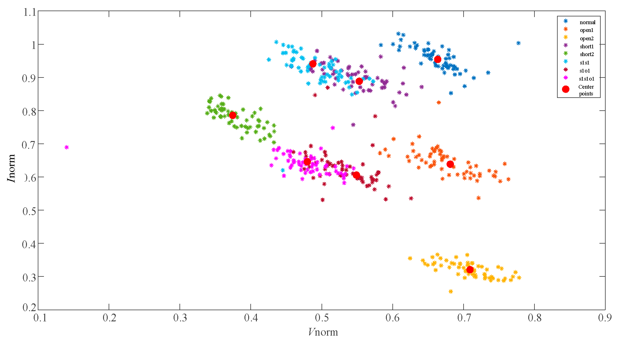
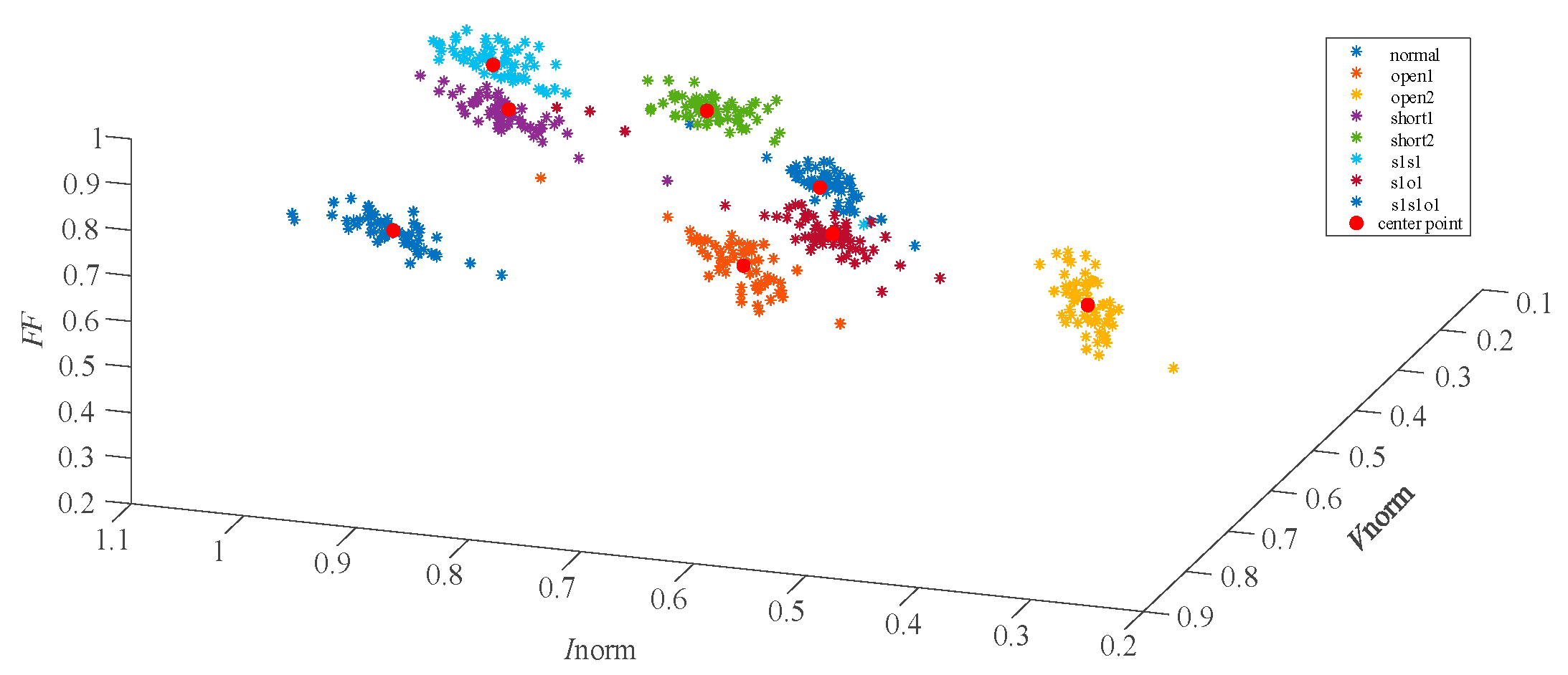
The eigenvector distribution of 8 fault types shown in Figure 9 indicates that some single faults and compound faults with similar characteristics are difficult to be discriminated in two-dimension space . In contrast, the feature vectors that are shown distributed in Figure 10 can yield a more obvious discrimination of 8 fault types than the eigenvectors . After the training process of GKFCM, the kernels of the 8 fault training datasets with two-dimension and three-dimension feature characteristics were calculated and distributed as the red points in Figure 9 and Figure 10, respectively.
In the fault identification phase of GKFCM, 120 samples of each fault are used to validate the effectiveness of the algorithm. The Equation (8) was used to calculate the similarity between the new fault data and the core points of the reference fault datasets. was set as 0.5. The results of fault diagnosis are listed in Table 7; Table 8, respectively. The Table 7 is the results acquired by processing two-dimension datasets and the Table 8 are the diagnostic performance that representing the processing results of the three-dimension fault datasets. In two tables, the first 8 faults in belong to the corresponding categories. In addition, line to line fault was defined as an unknown fault for validating the ability of the algorithm to identify an unknown faults. The diagnostic results in the last row of Table 7 and Table 8 illustrate that the proposed method based on GKFCM can also identify the unknown fault accurately.
It can be seen in Table 7 and Table 8 that all 8 fault types within the training datasets and the unknown faults realize fine discrimination. The results of this experiment demonstrate that the proposed algorithm has a good diagnostic performance for 8 common faults, including 5 single faults and 3 compound faults in PV array.
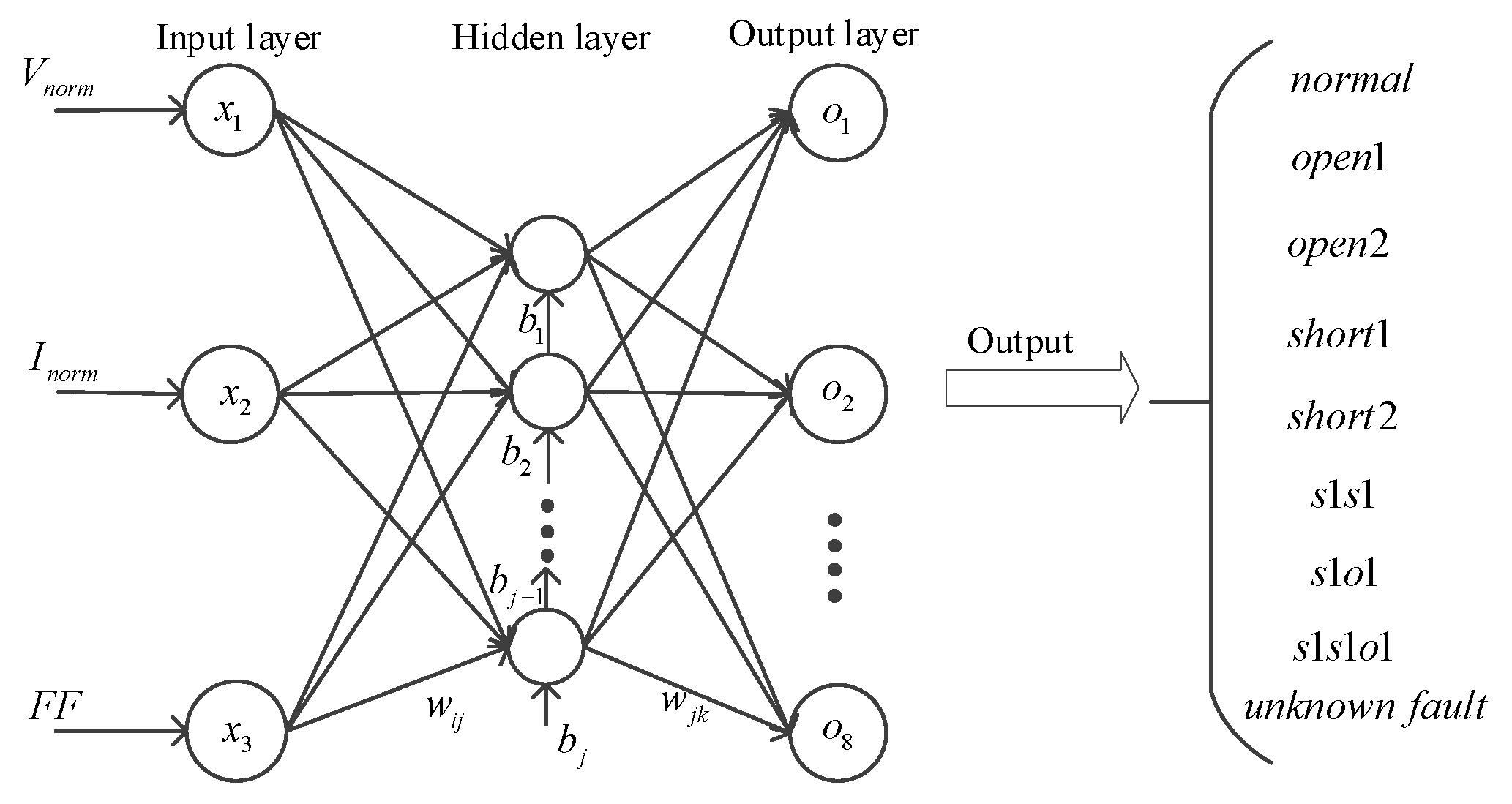
In order to further validate the persuasive and reliability of the proposed clustering method, a three-layer BP neural network was built to detect the 8 faults and an unknown fault. The structure of the BP neural network is shown in Figure 11. The BP neural network was trained by using the training datasets including 8 fault types, then the remaining fault samples of 8 fault types and the unknown fault samples were diagnosed by the trained BP neural network in the testing phase. The specific diagnostic results respectively characterized by two-dimension and three-dimension eigenvectors are shown in Table 9 and Table 10. The parameters in the BP neural network were set as follows: the iteration number was 1000, the learning rate was set as 0.01 and the minimum error was 0.01.
In the testing stage, two-dimension eigenvectors were used to characterize the 8 fault types and the unknown faults. The corresponding results are shown in Table 9.
Meanwhile, three-dimension eigenvectors were used to characterize the 8 fault types and the unknown faults. The final results are shown in Table 10.
In comparation with the results shown in Table 8 and Table 10, the processing algorithm with the two-dimension eigenvector has a lower diagnostic accuracy, and the details are shown in Table 7 and Table 9. These results demonstrate that the three-dimensional feature vectors, including the extended 3rd-dimension feature quantity, do improve the diagnostic accuracy of the faults.
In addition, compared to the results shown in Table 7 and Table 8, the performance of the BP neural network shown in Table 9 and Table 10 for the 8 known faults was similar to the results acquired by the proposed algorithm. However, the unknown faults are all identified as normal when the unknown faults occur. In respect to the detection of the unknown faults, the BP neural network has poor generalization ability. In contrast, the detection method based on GKFCM still has a relatively better diagnostic result when the unknown faults occur.
Overall, the results of the simulation and field experiments demonstrate that the strategy combining the new three-dimension eigenvectors and GKFCM proposed in this paper does not only exhibit a good diagnostic accuracy on the existing 8 fault types in the training datasets, but also can identify the unknown faults well. The algorithm presented has a good diagnostic accuracy and generalization capability.
7. Conclusions
A promising architecture to detect 8 faults of a PV array has been presented. This diagnostic strategy comprises the new feature eigenvector, including three new feature quantities and the GKFCM. The new feature vectors, including the normalized PV voltage, the normalized PV current and the fill factor, are proposed in the paper to discriminate 5 single faults and 3 compound faults with similar characteristics. The simulation and field experiments demonstrate that the proposed new eigenvectors have a good clustering ability and can differentiate 8 fault types in wide-weather conditions. Since the acquired fault datasets are accompanied by external and internal noise, the GKFCM was adopted to cluster the acquired fault datasets. The GKFCM uses the nonlinear kernel function to map the original feature space to the high-dimensional feature space and then clusters the fault datasets distributed in the high-dimensional space. The mapping procedure can highlight the feature differences of the different fault samples and effectively improve the clustering performance of the complex datasets. In the GKFCM, the similarity function in the support vector machine (SVM) is used as the fault classification function. The diagnostic results validate that the designed similarity function can classify the different faults very well. Finally, the simulation and field experiments were designed to verify the feasibility and effectiveness of the proposed algorithm.
Author Contributions
S.L. wrote the manuscript and analyzed the fault data. L.D and X.L. reviewed the manuscript. X.C. built the experiment platform. X.W. implemented the experiment and acquired the 8 fault datasets.
Funding
This research received no external funding.
Conflicts of Interest
The authors declare no conflict of interest.
References
- Takashima, T.; Yamaguchi, J.; Otani, K.; Kato, K.; Ishida, M. Experimental Studies of Failure Detection Methods in PV Module Strings. In Proceedings of the IEEE World Conference on Photovoltaic Energy Conference, Waikoloa, HI, USA, 7–12 May 2006. [Google Scholar]
- Takashima, T.; Yamaguchi, J.; Ishida, M. Disconnection detection using earth capacitance measurement in photovoltaic module string. Prostate 2008, 16, 669–677. [Google Scholar] [CrossRef]
- Hu, Y.; Cao, W.; Ma, J.; Finney, S.J.; Li, D. Identifying PV Module Mismatch Faults by a Thermography-Based Temperature Distribution Analysis. IEEE Trans. Device Mater. Reliab. 2014, 14, 951–960. [Google Scholar] [CrossRef]
- Gokmen, N.; Karatepe, E.; Silvestre, S.; Celik, B.; Ortega, P. An efficient fault diagnosis method for PV systems based on operating voltage-windows. Energy Convers. Manag. 2013, 73, 350–360. [Google Scholar] [CrossRef]
- Madeti, S.R.; Singh, S.N. Online fault detection and the economic analysis of grid-connected photovoltaic systems. Energy 2017, 134, 121–135. [Google Scholar] [CrossRef]
- Chouder, A.; Slivestre, S. Automatic supervision and fault detection of PV systems based on power losses analysis. Energy Convers. Manag. 2010, 51, 1929–1937. [Google Scholar] [CrossRef]
- Alam, M.K.; Khan, F.; Johnson, J.; Flicker, J. A Comprehensive Review of Catastrophic Faults in PV Arrays: Types, Detection, and Mitigation Techniques. IEEE J. Photovol. 2015, 5, 982–997. [Google Scholar] [CrossRef]
- Mellit, A.; Tina, G.M.; Kalogirou, S.A. Fault detection and diagnosis methods for photovoltaic systems: A review. Renew. Sustain. Energy Rev. 2018, 91, 1–17. [Google Scholar] [CrossRef]
- Lu, S.; Phung, B.T.; Zhang, D. A comprehensive review on DC arc faults and their diagnosis methods in photovoltaic systems. Renew. Sustain. Energy Rev. 2018, 89, 88–98. [Google Scholar] [CrossRef]
- Yao, X.; Herrera, L.; Ji, S.; Zou, K.; Wang, J. Characteristic Study and Time-Domain Discrete- Wavelet-Transform Based Hybrid Detection of Series DC Arc Faults. IEEE Trans. Power Electron. 2014, 29, 3103–3115. [Google Scholar] [CrossRef]
- Chen, S.; Li, X.; Xiong, J. Series Arc Fault Identification for Photovoltaic System Based on Time-Domain and Time-Frequency-Domain Analysis. IEEE J. Photovol. 2017, 7, 1105–1113. [Google Scholar] [CrossRef]
- He, C.; Mu, L.; Wang, Y. The Detection of Parallel Arc Fault in Photovoltaic Systems Based on a Mixed Criterion. IEEE J. Photovol. 2017, 7, 1–8. [Google Scholar] [CrossRef]
- Yi, Z.; Etemadi, A.H. Line-to-Line Fault Detection for Photovoltaic Arrays Based on Multiresolution Signal Decomposition and Two-Stage Support Vector Machine. IEEE Trans. Ind. Electron. 2017, 64, 8546–8555. [Google Scholar] [CrossRef]
- Yi, Z.; Etemadi, A. Fault Detection for Photovoltaic Systems Based on Multi-resolution Signal Decomposition and Fuzzy Inference Systems. IEEE Trans. Smart Grid 2016, 8, 1274–1283. [Google Scholar] [CrossRef]
- Chouay, Y.; Ouassaid, M. An intelligent method for fault diagnosis in photovoltaic systems. In Proceedings of the International Conference on Electrical and Information Technologies, Rabat, India, 15–18 November 2017. [Google Scholar]
- Wang, L.; Liu, J.; Guo, X.; Yang, Q.; Yan, W. Online fault diagnosis of photovoltaic modules based on multi-class support vector machine. In Proceedings of the Chinese Automation Congress, Jinan, China, 20–22 October 2017. [Google Scholar]
- Zhao, Y.; Ball, R.; Mosesian, J.; de Palma, J.F.; Lehman, B. Graph-Based Semi-supervised Learning for Fault Detection and Classification in Solar Photovoltaic Arrays. IEEE Trans. Power Electron. 2014, 30, 2848–2858. [Google Scholar] [CrossRef]
- Lin, P.; Lin, Y.; Chen, Z.; Wu, L.; Chen, L.; Cheng, S. A Density Peak-Based Clustering Approach for Fault Diagnosis of Photovoltaic Arrays. Int. J. Photoenergy 2017, 2017, 1–14. [Google Scholar] [CrossRef]
- Rui, B.; Ming, D.; Zhicheng, X.; Hu, G.; Danqi, Y. PV array fault diagnosis based on FCM. Acta Energiae Sol. Sin. 2016, 37, 730–736. [Google Scholar]
- Wang, J.; Rong, J.; Bo, T. Fault Diagnosis of Wind Turbine’s Gearbox based on EEMD and Fuzzy C Means Clustering. Acta Energiae Sol. Sin. 2015, 36, 319–324. [Google Scholar]
- Jingwei, L.; Meizhi, X. Kernelized Fuzzy Attribute C-means Clustering Algorithm. Fuzzy Sets Syst. 2008, 159, 2428–2445. [Google Scholar]
- Yiquan, W.; Yabing, H.; Shihua, W.; Yufei, Z.; Qiankun, X. Marine spill oil SAR image segmentation based on KFCM and improved CV model. Chin. J. Sci. Instrum. 2012, 33, 2812–2818. [Google Scholar]
- Jiang, Q.S.; Jia, M.P.; Hu, J.Z.; Xu, F.Y. A New Artificial Immunity Based Fuzzy Kernel Clustering Algorithm. China Mech. Eng. 2008, 5, 594–597. [Google Scholar]
- Baohai, H.; Yan, L.; Dongfeng, W. Steam Turbine Fault Diagnosis Based on KPCA and KFCM Ensemble. Electr. Power Autom. Equip. 2010, 7, 84–87. [Google Scholar]
- Li, Z.; Liu, Y.; Teng, W.; Yang, L. Fault diagnosis of Wind Power Gearbox Based on the KFCM trained by particle swarm optimization algorithm. J. Vibr. Meas. Diagn. 2017, 37, 484–488. [Google Scholar]
- Mei, F.; Mei, J.; Zheng, J.; Zhang, S.; Zhu, K. Application of Particle Swarm Fused KFCM and Classification Model of SVM for Fault Diagnosis of Circuit Breaker. Proc. CSEE 2013, 33, 134–141. [Google Scholar]
- Hariharan, R.; Chakkarapani, M.; Ilango, G.S.; Nagamani, C. A Method to Detect Photovoltaic Array Faults and Partial Shading in PV Systems. IEEE J. Photovol. 2016, 6, 1278–1285. [Google Scholar] [CrossRef]
- Ma, H.; Ekanayake, C.; Saha, T.K. Power transformer fault diagnosis under measurement originated uncertainties. IEEE Trans. Dielectr. Electr. Insul. 2012, 19, 1982–1990. [Google Scholar] [CrossRef]
- Ma, T.; Yang, H.; Lu, L. Development of a model to simulate the performance characteritics of crystalline silicon photovoltaic modules/strings/arrays. Sol. Energy 2014, 100, 31–41. [Google Scholar] [CrossRef]
- Ventura, C.; Tina, G.M. Utility scale photovoltaic plant indices and models for on-line monitoring and fault detection purposes. Electr. Power Syst. Res. 2016, 136, 43–56. [Google Scholar] [CrossRef]
Figure 1.
The flow chart of the fault diagnostic method based on Gaussian Kernel Fuzzy C-means clustering method (GKFCM).
Figure 1.
The flow chart of the fault diagnostic method based on Gaussian Kernel Fuzzy C-means clustering method (GKFCM).

Figure 2.
The simulation model of PV array.

Figure 3.
The distribution of the 8 fault characteristic points .

Figure 4.
The distribution of the 8 fault characteristic points .

Figure 5.
The distribution of the 8 faults characteristic points .

Figure 6.
The training datasets and clustering center points of 8 faults.

Figure 7.
The platform of PV array.

Figure 8.
The solar irradiance and temperature range in the whole day on 7 September 2018.


Figure 9.
The distribution of eight fault characteristic points in the field experiment.

Figure 10.
The distribution of eight fault characteristic points and clustering center points in the field experiment.
Figure 10.
The distribution of eight fault characteristic points and clustering center points in the field experiment.

Figure 11.
Basic structure of the BP neural network.


Table 1.
Key parameters of JW-G2300-MD6660P-1 photovoltaic (PV) Module.
| Description | Value |
|---|---|
| Maximum power () | 230.3 W |
| Maximum power point voltage in STC () | 31.00 V |
| Maximum power point current in STC () | 7.430 A |
| Open circuit voltage in STC () | 37.10 V |
| Short circuit current in STC () | 8.050 A |
| Temp. dependence of () | 0.04350 |
| Temp. dependence of () | −0.3515 |
| Number of cells in series () | 60.00 |
Table 2.
Eight fault categories description.
| Fault Types | Descriptions | Labels |
|---|---|---|
| Case 1 | no faults | normal |
| Case 2 | one string in open-circuit condition | open1 |
| Case 3 | two string in open-circuit condition | open2 |
| Case 4 | one module in short-circuit condition | short1 |
| Case 5 | two modules distributed in one string in short-circuit condition | short2 |
| Case 6 | two modules distributed in two different strings respectively in short-circuit condition | s1s1 |
| Case 7 | one module in short-circuit condition and another string in open-circuit condition | s1o1 |
| Case 8 | two modules distributed in two different strings respectively in short-circuit condition and the other string is in open-circuit condition | s1s1o1 |
Table 3.
The range of environmental parameters in simulation experiment.
| Datasets | Irradiance/W·m−2 | Temperature/°C |
|---|---|---|
| Training datasets | 200 | 0–20 |
| Testing datasets | 450–900 | 10–20 |
Table 4.
Center-point coordinates of 8 clusterings in the reference fault datasets.
| Fault Types | Labels | Coordinates |
|---|---|---|
| case 1 | normal | (0.8691, 0.9268, 0.8053) |
| case 2 | open1 | (0.8685, 0.6178, 0.8049) |
| case 3 | open2 | (0.8682, 0.3089, 0.8044) |
| case 4 | short1 | (0.6843, 0.9316, 0.8020) |
| case 5 | short2 | (0.4569, 0.9368, 0.8071) |
| case 6 | s1s1 | (0.6639, 0.9292, 0.8061) |
| case 7 | s1o1 | (0.6718, 0.6200, 0.8048) |
| case 8 | s1s1o1 | (0.6524, 0.6174, 0.8052) |
Table 5.
Eight fault identification accuracy in testing phase of simulation experiment.
| Fault Types | Sample Number for Identification | Identified Sample Number |
|---|---|---|
| normal | 110 | 110 |
| open1 | 110 | 110 |
| open2 | 110 | 110 |
| short1 | 110 | 110 |
| short2 | 110 | 110 |
| s1s1 | 110 | 110 |
| s1o1 | 110 | 110 |
| s1s1o1 | 110 | 110 |
Table 6.
Key specifications of GSP-240 PV Module.
| Description | Value |
|---|---|
| Maximum power () | 240.0 W |
| Maximum power point voltage in STC () | 37.60 V |
| Maximum power point current in STC () | 8.540 A |
| Open circuit voltage in STC () | 29.60 V |
| Short circuit current in STC () | 8.110 A |
| Temp. dependence of () | 0.1750 |
| Temp. dependence of () | −0.4882 |
| Number of cells in series () | 60.00 |
Table 7.
Eight fault and unknown fault identification accuracy in testing phase of the field experiment.
Table 7.
Eight fault and unknown fault identification accuracy in testing phase of the field experiment.
| Fault Types | Sample Number for Identification | Identified Sample Number |
|---|---|---|
| normal | 120 | 118 |
| open1 | 120 | 119 |
| open2 | 120 | 119 |
| short1 | 120 | 72 |
| short2 | 120 | 116 |
| s1s1 | 120 | 67 |
| s1o1 | 120 | 79 |
| s1s1o1 | 120 | 66 |
| unknown fault | 120 | 0 |
Table 8.
Eight fault and an unknown fault identification accuracy in testing phase of the field experiment.
Table 8.
Eight fault and an unknown fault identification accuracy in testing phase of the field experiment.
| Fault Types | Sample Number for Identification | Identified Sample Number |
|---|---|---|
| normal | 120 | 120 |
| open1 | 120 | 117 |
| open2 | 120 | 119 |
| short1 | 120 | 109 |
| short2 | 120 | 117 |
| s1s1 | 120 | 101 |
| s1o1 | 120 | 117 |
| s1s1o1 | 120 | 102 |
| unknown fault | 120 | 0 |
Table 9.
Eight faults and unknown fault identification accuracy in testing phase of the field experiment.
Table 9.
Eight faults and unknown fault identification accuracy in testing phase of the field experiment.
| Fault Types | Sample Number for Identification | Identified Sample Number |
|---|---|---|
| normal | 120 | 117 |
| open1 | 120 | 117 |
| open2 | 120 | 119 |
| short1 | 120 | 73 |
| short2 | 120 | 112 |
| s1s1 | 120 | 55 |
| s1o1 | 120 | 58 |
| s1s1o1 | 120 | 96 |
| unknown fault | 120 | all identified as normal |
Table 10.
Eight faults and the unknown fault identification accuracy in testing phase of the field experiment.
Table 10.
Eight faults and the unknown fault identification accuracy in testing phase of the field experiment.
| Fault Types | Sample Number for Identification | Identified Sample Number |
|---|---|---|
| normal | 120 | 118 |
| open1 | 120 | 117 |
| open2 | 120 | 119 |
| short1 | 120 | 115 |
| short2 | 120 | 116 |
| s1s1 | 120 | 104 |
| s1o1 | 120 | 117 |
| s1s1o1 | 120 | 101 |
| unknown fault | 120 | all identified as normal |
© 2019 by the authors. Licensee MDPI, Basel, Switzerland. This article is an open access article distributed under the terms and conditions of the Creative Commons Attribution (CC BY) license (http://creativecommons.org/licenses/by/4.0/).
Share and Cite
MDPI and ACS Style
Liu, S.; Dong, L.; Liao, X.; Cao, X.; Wang, X. Photovoltaic Array Fault Diagnosis Based on Gaussian Kernel Fuzzy C-Means Clustering Algorithm. Sensors 2019, 19, 1520. https://doi.org/10.3390/s19071520
AMA Style
Liu S, Dong L, Liao X, Cao X, Wang X. Photovoltaic Array Fault Diagnosis Based on Gaussian Kernel Fuzzy C-Means Clustering Algorithm. Sensors. 2019; 19(7):1520. https://doi.org/10.3390/s19071520
Chicago/Turabian StyleLiu, Shengyang, Lei Dong, Xiaozhong Liao, Xiaodong Cao, and Xiaoxiao Wang. 2019. "Photovoltaic Array Fault Diagnosis Based on Gaussian Kernel Fuzzy C-Means Clustering Algorithm" Sensors 19, no. 7: 1520. https://doi.org/10.3390/s19071520
Note that from the first issue of 2016, this journal uses article numbers instead of page numbers. See further details here.