Measurement of Atmospheric Dimethyl Sulfide with a Distributed Feedback Interband Cascade Laser


State Key Laboratory of Precision Measuring Technology and Instruments, Tianjin University, Tianjin 300072, China
*
Author to whom correspondence should be addressed.
Sensors 2018, 18(10), 3216; https://doi.org/10.3390/s18103216
Submission received: 14 August 2018
/
Revised: 14 September 2018
/
Accepted: 18 September 2018
/
Published: 24 September 2018
(This article belongs to the Special Issue VOC Sensors Applicable to IoT and Healthcare)
Abstract
:This paper presents a mid-infrared dimethyl sulfide (CH3SCH3, DMS) sensor based on tunable laser absorption spectroscopy with a distributed feedback interband cascade laser to measure DMS in the atmosphere. Different from previous work, in which only DMS was tested and under pure nitrogen conditions, we measured DMS mixed by common air to establish the actual atmospheric measurement environment. Moreover, we used tunable laser absorption spectroscopy with spectral fitting to enable multi-species (i.e., DMS, CH4, and H2O) measurement simultaneously. Meanwhile, we used empirical mode decomposition and greatly reduced the interference of optical fringes and noise. The sensor performances were evaluated with atmospheric mixture in laboratory conditions. The sensor’s measurement uncertainties of DMS, CH4, and H2O were as low as 80 ppb, 20 ppb, and 0.01% with an integration time 1 s, respectively. The sensor possessed a very low detection limit of 9.6 ppb with an integration time of 164 s for DMS, corresponding to an absorbance of 7.4 × 10⁻⁶, which showed a good anti-interference ability and stable performance after optical interference removal. We demonstrated that the sensor can be used for DMS measurement, as well as multi-species atmospheric measurements of DMS, H2O, and CH4 simultaneously.
1. Introduction
Dimethyl sulfide (CH3SCH3, DMS) is a poisonous and easily explosive volatile organic sulfur compound, which originates not only from numerous production and consumption processes of phytoplankton within the marine eco-system, but also comes from the emissions of volcanoes and vegetation [1,2,3,4]. Moreover, it is a component of the smell produced from cooking certain vegetables, notably maize, cabbage, beetroot and seafood. Thus, DMS exists widely on the ocean’s surface as well as in the atmosphere [5,6,7]. DMS primarily comes from dimethyl sulfoniopropionate, a major secondary metabolite in some marine algae, and oxidized in the marine atmosphere to various sulfur-containing compounds, such as sulfur dioxide, dimethyl sulfoxide, dimethyl sulfone, methanesulfonic acid and sulfuric acid [8,9]. Among these compounds, sulfuric acid has the potential to create new aerosols which act as cloud condensation nuclei; through this interaction with cloud formation, the massive production of atmospheric DMS over the oceans may have a significant impact on the Earth’s climate [10,11,12]. Furthermore, DMS has an odor threshold value that varies from 0.6 to 40 ppb (parts per billion) between different persons and it is highly flammable and irritant to eyes and skin with concentration more than 1 ppm (parts per million) [13,14,15]. In conventional municipal wastewater treatment, incubation of activated sludge has 1–10 mg/L dimethyl sulfoxide produced dimethyl sulfide (DMS) in the headspace gas, a concentrations that exceeded the odor threshold by approximately four orders of magnitude [16]. The concentration of DMS in natural gas field is about 1.8 ppm. Moreover, it is about 6.5 ppm in the exhaust fumes from the chemical plant [17]. Therefore, it is necessary to monitor DMS continuously from ppb to ppm levels for the purpose of environmental protection as well as human safety.
Common methods for detecting DMS include Tunable Laser Absorption Spectroscopy (TLAS) [13], Gas Chromatography (GC) [18], Gas Chromatography-Mass Spectrometry (GC-MS) [19], chemical gas sensors [20,21], Gas Chromatography–Flame Photometric Detection (GC-FPD) [22,23], Fourier Transform Infrared Spectrometer (FTIR) [24], etc. However, whether GC, GC-MS, or GC-FPD, although they have a detection limit down to ppb or ppt (parts per trillion) levels, the DMS should be collected with material resistant to adsorption and oxidation. Furthermore, it requires a complex pre-treatment procedure. These methods are either costly or have a short lifetime. Chemical gas sensors such as ZnO gas sensor are made and tested for concentration as low as 2 ppm of DMS [20]. However, the processing and production steps of ZnO gas sensor are very complicated, and the accuracy of the sensor is affected by ambient humidity. FTIR is used to perform rapid measurement of DMS [24]. However, FTIR is often frustrated by interference from water and carbon dioxide for low spectral resolution. TLAS is a promising technique for trace gas measurement in situ or on line, which is usually used to modulate laser and scan the spectral line; thus, we can get the absorption line of molecules. It can not only realize point sampling measurement with a multi-pass gas cell, but can also be used for remote monitoring with open optical path.
Recently, a Mid-Infrared (MIR) spectral DMS sensor was developed by our group [13]. The sensor boasted a very high sensitivity of 20 ppb with working wavelength of 3367.3 nm located at the ν14/ν18-band of DMS. However, it was balanced by pure nitrogen and only DMS was detected, rather than a real air condition. Although spectral interference has been considered comprehensively during spectra investigation, practically, the sensitivity of the sensor is deteriorated by the strong spectral interference from H2O and CH4 when working in practical air condition; there is no other method of data processing for reducing the interference of optical fringes and noise; and the accuracy is affected by internal optical path.
Moreover, based on our previous investigation, the atmospheric DMS concentration is about 28 ppb around a sewage treatment tower and about 500 ppb near an instant noodle factory. Thus, in this paper, to develop a DMS sensor with strong anti-interference capability and stable performances to detect polluted atmosphere in those factories and the surrounding environment, we utilized another candidate spectrum with wavelength of 3336.7 nm located at the ν1/ν8-band of DMS, and deduced the concentration of DMS, as well as atmospheric interference CH4 and H2O simultaneously by Multi-Component Spectral Fitting (MCSF). Moreover, we reduced the interference from noise and optical fringes by performing Empirical Mode Decomposition (EMD) and reconstruction to the recorded spectral data. The sensor’s performances were evaluated with common air mixture in laboratory conditions.
2. Sensor Configuration
We developed a DMS sensor based on wavelength modulation spectroscopy, whose theoretical basis is the Beer-Lambert absorption law [25,26,27,28,29,30,31,32]. When the absorbance A < 0.05, according to Beer-Lambert absorption law and optically thin condition, absorption coefficient is an even periodic function in ωt and can be expanded as a Fourier cosine series:
where is the central frequency of laser; a is the modulation amplitude, which is the wavelength modulation of the laser generated by sinusoidal modulation; ω is the modulation frequency; Hk are Fourier series; and k is the harmonic order. Because the second harmonic signal 2f is closely related to the absorption and free of background, typically k = 2 is used in Wavelength Modulation Spectroscopy (WMS). Thus, for the mixed second harmonic signal of n types of gases, they can be expressed as follows:
where P is the pressure, L is the length of optical path, χi is the mole fraction of the ith absorbing species, and Sij and φij are the line strength and line shape function of the jth line of the ith absorbing species, respectively. Referring to Equation (2), if the pressure and temperature remain constant, we can ignore the variations of line profile, and it can be expressed as:
where is the second harmonic signal of the ith absorbing species in per unit volume concentration, and the magnitude of the absorption-based 2f signal, , which is usually measured by a lock-in amplifier, and described as [23]:
where S2f is the 2f signal that is measured by a lock-in amplifier, G is the electro-optical gain of the measurement system, Io is average intensity of the laser at frequency , and S2f_i_per is the 2f signal of ith absorbing species in per unit volume concentration. Therefore, S2f of a mixture theoretically equals the sum of the product of each component’s concentration and its 2f signal in per unit volume concentration.
2.1. Working Spectral Band Selecting
The MIR fundamental absorption spectra of DMS were investigated in detail in our previous work [13]. By compromise of the absorption intensity, spectral line interference, and convenient laser wavelength, the spectral range located at ν14/ν18-bandwidth wavelength of 3367.3 nm was preferred, and the strong absorption made the sensor possess much higher measurement sensitivity than other spectral lines.
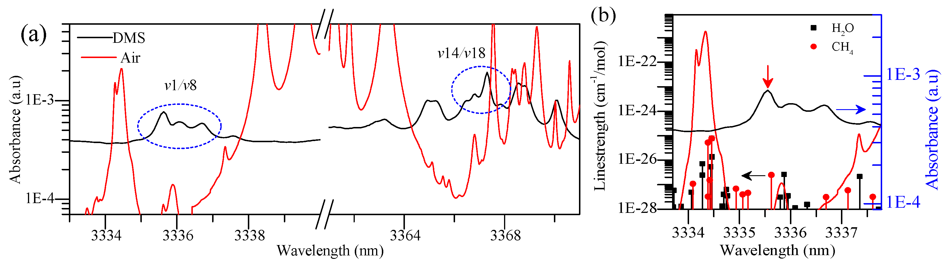
We reexamined the spectral line of DMS based on minimum interference principle, including relatively less interference lines and distant interference spectral lines, and the absorbance of absorption line is relatively large. Thus, another spectral range of DMS was preferred based on the Pacific Northwest National Laboratory (PNNL) and High Resolution Transmission (HITRAN) databases. The 5 ppm×m DMS within the range of 3333–3371 nm is presented in Figure 1a,b.
Figure 1a shows the two regions possible for the measurement of DMS, and Figure 1b is the spectrum located at ν1/ν8-band to be measured. Detailed analysis is presented in Table 1.
The absorption peak wavelength and strength of DMS candidate regions are listed as well as the spectral information of possible interferences from air absorptions. In Figure 1a,b and Table 1, there are about three main absorption peaks at the ν1/ν8-band between 3333.7 and 3337.8 nm, and the ν1/ν8-band of 3336.710 nm suffers much lower interference than ν14/ν18-band of 3367.229 nm, including the magnitude of interference and distance between the absorption line and the interference line. Thus, we chose 3333.7–3337.8 nm as our ultimate selection for DMS measurement with comprehensive consideration. Furthermore, although CH4 and H2O have less interference in the absorption of DMS, they are located at the working range of the laser. At the same time, the absorption spectra of methane and water overlap each other, thus it is necessary to obtain the concentration of three gases simultaneously by using the MCSF.
2.2. Setup
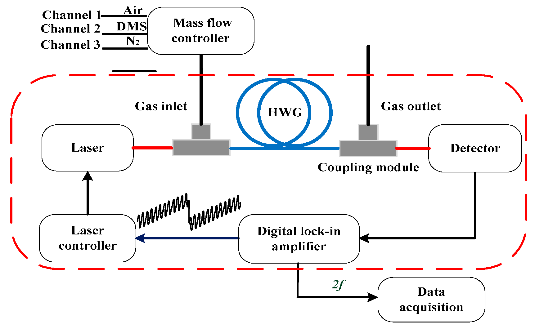
We developed a DMS gas sensor based on our instrument development platform [25,33,34,35], which consists of a homemade digital lock-in amplifier with signal generation function, a laser controller, a DFB-ICL, a hollow waveguide (HWG), and a photodetector. The schematic plot of the sensor is shown in Figure 2. The digital lock-in amplifier sent out a high frequency modulation signal to the laser controller (ILX Lightwave, Irvine, CA, USA, LDC-3908); the DFB-ICL (Nanoplus GmbH, Gerburnn, Germany) with wavelength of 3337 nm was used as the optical source; and both the temperature and current of the laser were controlled by the laser controller. The beam emitted from the laser was aligned into the HWG (Polymicro Technologies, Brookfield, IL, USA, Type HWEA10001600), and then collected by the photodetector (Thorlabs, Newton, NJ, USA, PDA20H-EC). The converted electrical signal was sent to the homemade digital lock-in amplifier and demodulated. Through data acquisition software, the 2f signal was processed by MCSF program to obtain the target gas concentration.
We carefully set all the working parameters of the sensor, including the optical path, gas flow, modulation amplitude, temperature, and so on. The instantaneous line width, dynamic tuning rate, and slope efficiency of ICLs have been reported to be suitable for precision spectroscopy measurements [36]. The laser power before and after HWG were 5.5 mW and 0.9 mW, respectively. Effective optical path length of the HWG was 5 m and its volume was as small as 4.7 mL. The homemade mass flow controller was kept at 50 mL/min with consideration of reducing the influence of pressure changes inside the HWG. The laser controller was controlled by a 10 Hz sawtooth wave with amplitude of 1.45 V and a 2.56 kHz sinusoidal signal with a VPP of 75 mV, and set to 3.5 °C to cover the entire measurement area. At the same time, the digital lock-in amplifier provided a high frequency sinusoidal signal that is two times the frequency of the laser controller to demodulate the spectral signal from the photodetector. Finally, we obtained the 2f demodulation signal from the data acquisition software.
We optimized the modulation amplitude of the DFB-ICL to enable measurement of multi-species spectra without overlap. We optimized the modulation amplitude according to Spectral Discrimination (SD) and normalized amplitude of the DMS WMS-2f signal [26]. Traditional optimal modulation coefficient (2.2) [29] can no longer meet the requirements because of the interference of noise and optical fringes. Therefore, according to the cross of SD curve and normalized amplitude curve of the DMS WMS-2f signal, modulation amplitude of 0.27 cm−1 was chose as our optimized selection. Thus, the modulation amplitude of 0.27 cm−1 was preferred to improve the Signal-to-Noise Ratio (SNR) and measurement accuracy.
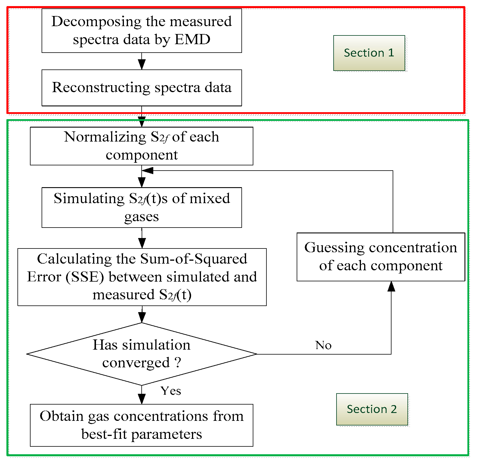
A MCSF algorithm to reduce spectral interference was developed in our previous work [25], as shown in Figure 3. The algorithm is an improved Levenberg-Marquardt (L-M) algorithm, which is based on nonlinear least squares curve-fitting algorithm [28]. In this algorithm, the reference signal of each component and their mixed signals are given first. Because the mixed signals equal the product of the concentration of each gas and their corresponding reference signals, we set the initial concentration of each component and through iterative method, we can get each component’s actual concentration. The algorithm first calculates the concentration of each gas, and then multiplies the corresponding pure absorption signal and sums them. Once the variance between the added mixed signal and the measured signal reaches the minimum, the algorithm converges. After that, the best fitting parameters were the concentrations of all components.
As for the wide-band characteristics of the MIR fingerprint absorption, the measurement sensitivity and accuracy are always deteriorated by overlap with adjacent spectrum, optical fringes, and noise. A solution by EMD and reconstruction to the recorded spectral data was developed in our previous work [26], as shown Section 1 in Figure 3. EMD decomposes the signal into a series of Intrinsic Mode Function (IMF) components; these components have different physical meanings. Thus, we can eliminate optical fringes and noise according to the characteristics of signal, and reconstruct the original signal. In view of the above, we combined the MCSF and EMD to calculate and optimize the multi-component concentration in a mixture. Steps of this algorithm are displayed in Figure 3.
The algorithm includes two parts: (1) EMD is used to decompose and reconstruct the measured spectral data for reducing the optical fringes and noise; and (2) the 2f signal of each component is normalized, the initialization concentration parameters of each component are estimated, and the 2f signals of single component concentration and mixed concentrations participating in the fitting are produced. If the algorithm converges, the best fitting parameters are obtained. In our simulation, the results of the algorithm basically did not depend on the initial concentration. When the concentration of DMS is within the range of 1–20 ppm, the algorithm always converges.
The initialization concentrations of DMS, methane, and water were set as 1 ppm, 1 ppm, and 1%, respectively. Each component used 370 points to participate in fitting, and the program usually cycles fewer than 100 times. Once the algorithm converges, the best fitting parameters are determined.
2.3. Reference WMS-2f Signal Acquisition for MCSF
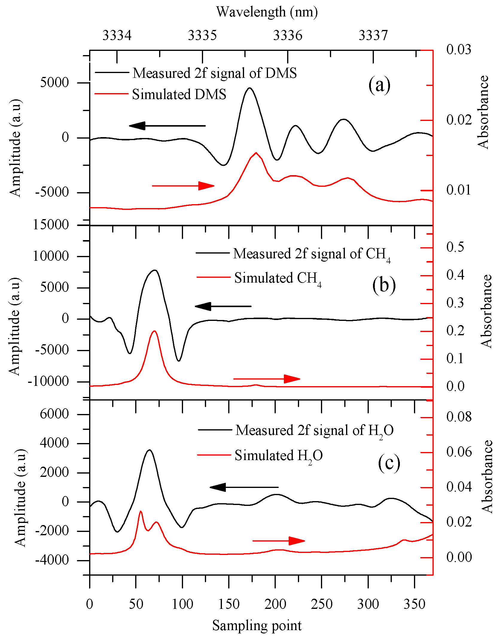
We obtained superior reference signals of DMS, CH4, and H2O for the MCSF algorithm of the sensor with elaborately planned experiments. The HWG was filled with N2 first and then with a reference gas, therefore, the difference between the 2f signals of the reference gas and N2 could be used as reference signal. The reference signals of DMS and CH4 were obtained using reference gases with concentrations of 20.2 ppm and 3 ppm, respectively. In contrast, the reference signal of H2O was obtained using high humidity air that subtracted air background, and the high humidity air was obtained by a humidifier. With the EMD method [26], we reduced the optical fringes and noise the most. Thus, the measured reference 2f signal of each component with less optical fringe and noise between 3333.7 and 3337.8 nm of DMS, CH4, and H2O are shown in Figure 4a–c, respectively.
2.4. Optical Fringes Removal
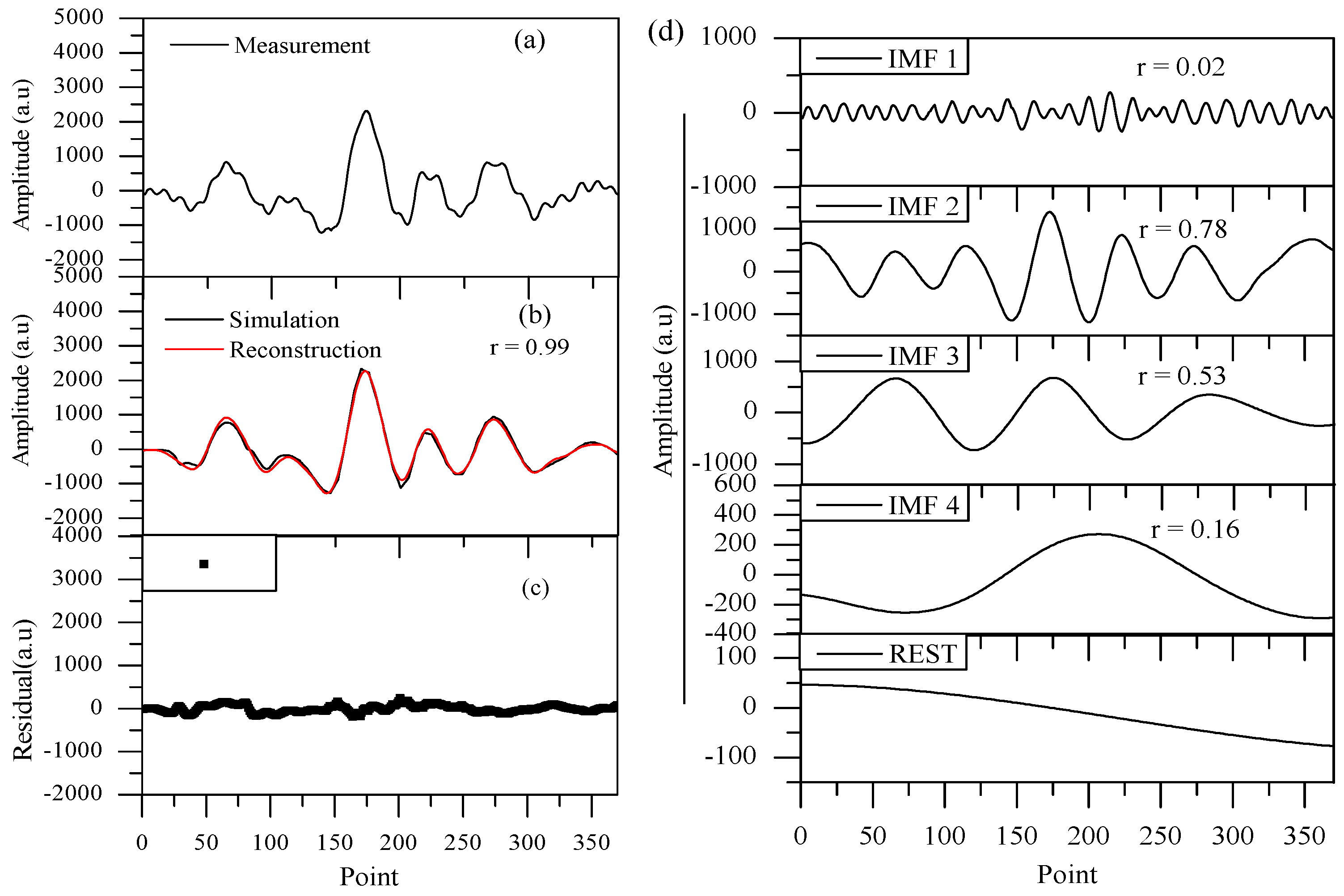
We reduced the interference from noise and optical fringes by decomposing the measured 2f signals of the mixture and reconstructing them with the EMD method. Take the mixture of H2O (0.14%)-CH4 (0.19 ppm)-DMS (10.1 ppm) as an example: about four IMF components were obtained. Thus, according to the signal characteristics of correlation coefficient, amplitude, and symmetry, the signal was reconstructed, as shown in Figure 5a–d.
Noise signals usually possess the characteristics of small amplitude and high frequency, while optical fringes are similar to the profile of sinusoidal signal, and all of them have a very low correlation coefficient relative to the absorption signal. Thus, IMF 1 in Figure 5d with a correlation coefficient r of 0.02 was diagnosed as mixture of noise and optical fringes with comprehensive consideration of amplitude, frequency, and correlation coefficient. IMF 2, IMF 3, IMF 4, and the rest of the signal made up the reconstructed absorption signal, as shown in Figure 5b. The reconstructed signal with a correlation coefficient of 0.99 meant that, in the process of decomposition and reconstruction, there was basically no loss or distortion of absorption information.
3. Sensor Performance Verification
3.1. Detection Ability
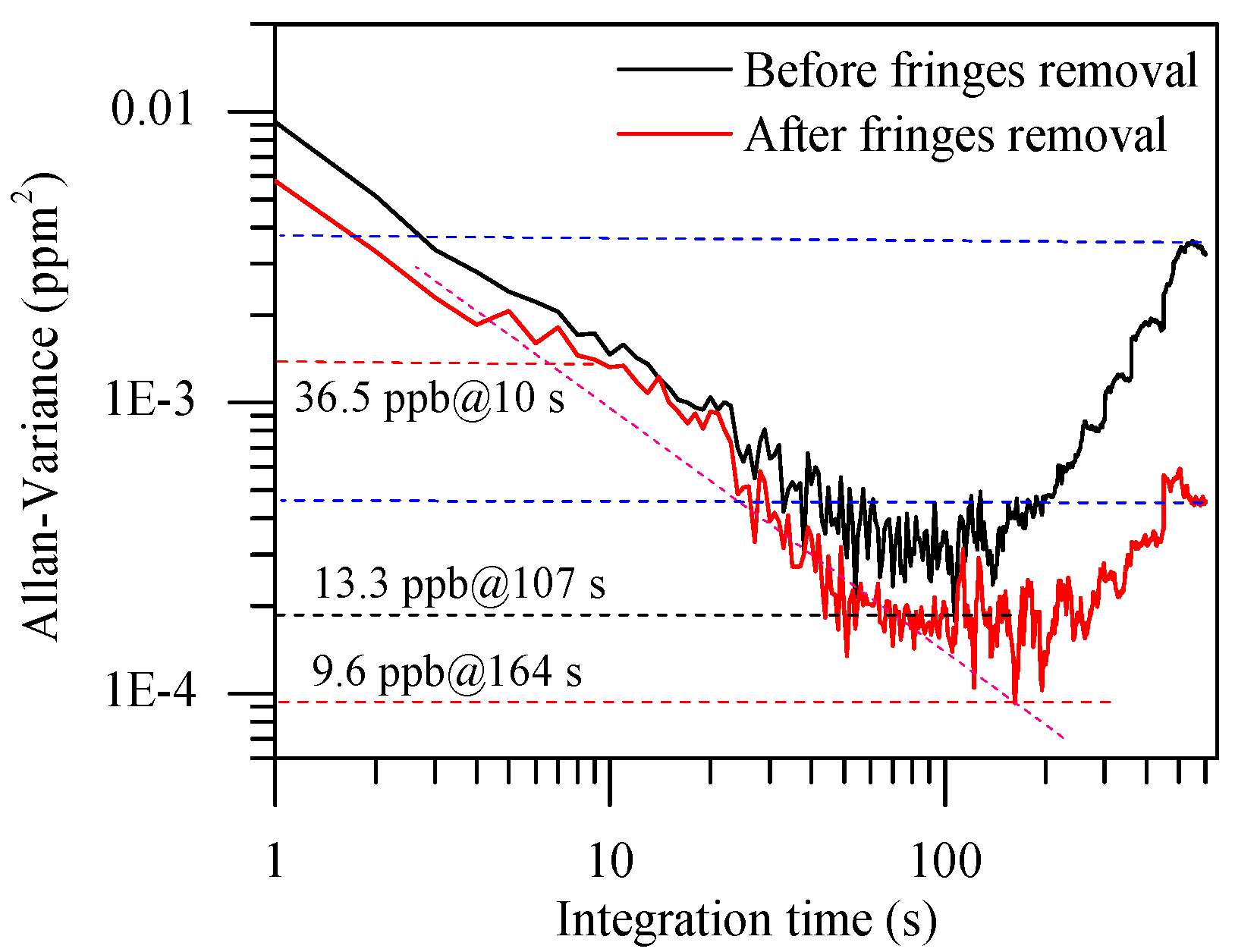
The detection ability of sensor was usually limited by noise and optical fringes [29,37]. Thus, we tested the detection ability of the sensor with reference gas of DMS before and after fringes removal. We performed EMD, signal reconstruction, and MCSF on recorded spectral signals, and then calculated the concentration of DMS. The calculated concentration was consistent with the nominal value of the reference gas. We evaluated the sensor’s detection ability by calculating the Allan variance of continuous DMS measurements for more than 30 min. To verify the enhancement effect of fringes removal using EMD method, we calculated and compared the Allan variance before and after fringes removal, as shown in Figure 6.
A comparison was made for the sensitivity and detection limit before and after fringe removal. In Figure 6, we can see that the sensor performances have been greatly enhanced, which presented in two aspects: (1) the minimum of the Allan variance reduced from 13.3 ppb (with integral time 107 s) to 9.6 ppb (with integral time 164 s), which means that the sensor’s detection limit significantly improved; and (2) the Allan variance reduced by an order of magnitude when integrated time increased to at least 500 s, as shown in Figure 6 (the two blue dotted lines), which means that the sensor’s long-term stability attained a distinguished improvement. After the removal of fringes, the sensitivity and detection limit of reconstructed signals were optimized at 20 ppb and 3.7 ppb compared to measured signals, respectively. Furthermore, the curve trend of fringes removal indicated that the sensor was much more stable than before, which benefited from the suppression of noise and optical fringes. As seen from the reconstructed signal, there was a detection limit of 9.6 ppb with an optimal integration time of 164 s for DMS, corresponding to an absorbance of 7.4 × 10⁻⁶, which is sufficient to satisfy the needs of human health. Although the detection limit is much lower than the 2.8 ppb mentioned in Reference [13], it is because of the relatively weak absorption. Actually, our spectral lines performed by EMD have more practical significance, and a greater anti-interference ability, which may also contribute the improvement of detection limit in reference [13].
3.2. Measurement Linearity and Uncertainty
Two groups of DMS concentration gradient experiments with air mixture (i.e., CH4 and H2O), prepared with a homemade high-precision gas mixer [38], were carried out to verify the sensor’s performance. The DMS was prepared with the Gravimetric Standards blending with nitrogen and verified with gas chromatography method [39]. The concentration of CH4 and H2O in the air were tested beforehand by absolute measurement of direct absorption spectroscopy. The initial concentrations of DMS, CH4, and H2O were 20.2 ppm, 1.9 ppm, and 1.4%, respectively. Thus: (1) in the first group, the concentration of DMS ranged from 2.02 to 10.1 ppm (in 2.02 ppm intervals), while the concentration of CH4 and H2O remained at 0.95 ppm and 0.7%, respectively; and (2) the concentration of CH4 ranged from 0.19 to 0.95 ppm (in 0.19 ppm), the concentration of H2O ranged from 0.14% to 0.7% (in 0.14% intervals), and the volume of DMS remained at 10.1 ppm in the second group. All of the concentration settings were realized by adjusting the three-channel volumetric flow rate settings in Figure 2. Specific reference concentration ratios are shown in Table 2 and Table 3. Each mixture was measured 10 times and the average was taken to reduce noise. The peak absorption of each mixture was estimated to be less than 0.05 and satisfied the optical thin condition of WMS. All experiments were performed at 1 atm.
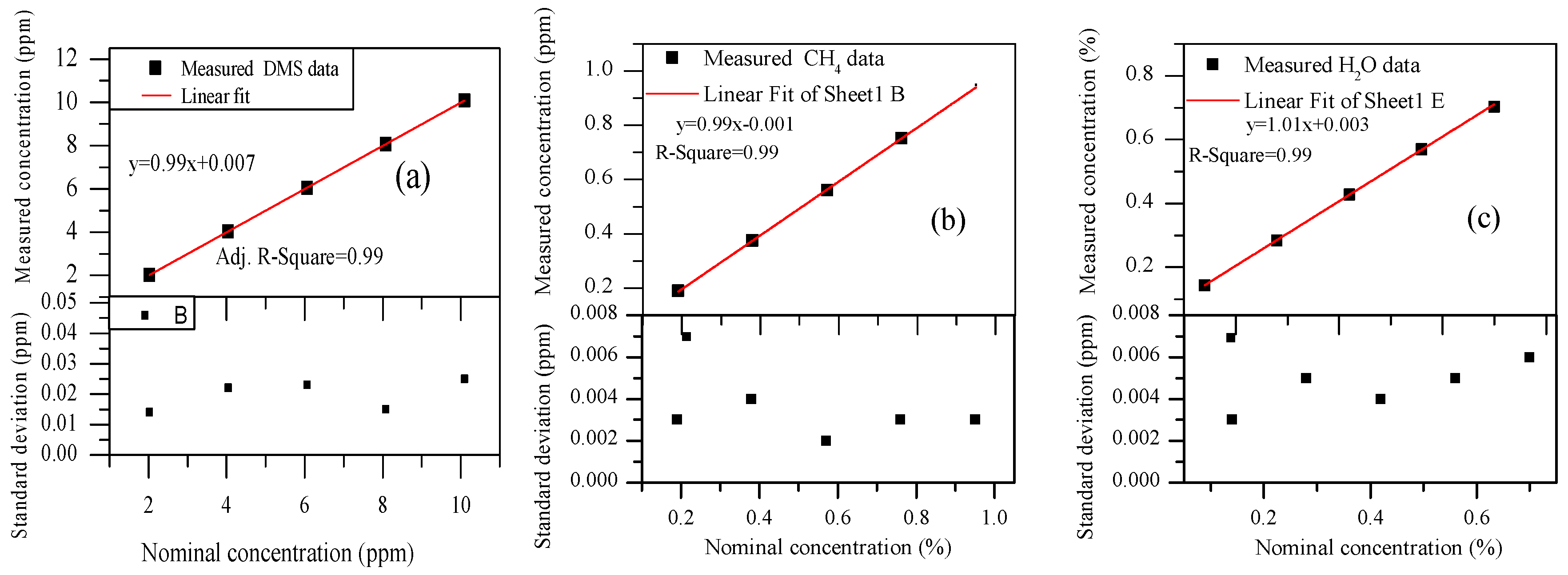
We measured and fitted the concentration of DMS in the first group, as shown in Figure 7a, and concentrations of CH4 and H2O in the second group, as shown in Figure 7b,c, whose concentrations changed in gradient in two groups of experiments. All experiments were carried out at room temperature.
The concentration of DMS, CH4, and H2O were measured, as shown in Figure 7a–c. The error bars represent the difference between the measured value and the true value. The square of correlation coefficient, R2, were all equal to 0.99, which showed a very good linear relationship between the measured concentration and nominal concentration (i.e., reference concentration) for DMS, CH4, and H2O. The measured accuracy of DMS, CH4, and H2O were 0.3%, 1.9%, and 2.8%, respectively. The standard deviations could primarily be attributed to the uncertainty of the mass flow controller and the fluctuation of H2O in the air over time. Although because of the concentration gradient, the O2 and N2 concentrations in the experiment are different from their actual concentrations in air, they have no absorption in the spectrum that we chose and have less influence on our measurement.
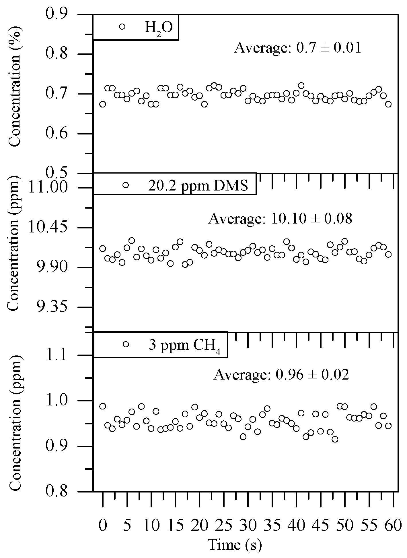
Sixty measurements with 1 s intervals were performed to verify the stability and accuracy of the sensor with the flowing gas mixture of 10.1 ppm DMS, 0.95 ppm CH4, and 0.7% H2O. The results are shown in Figure 8.
In Figure 8, the average concentrations of DMS, CH4, and H2O were 10.10 ± 0.08 ppm, 0.96 ± 0.02 ppm, and 0.7 ± 0.01% with a sampling interval of 1 s, respectively. Therefore, the measurement uncertainties of DMS, CH4, and H2O were 80 ppb, 20 ppb, and 0.01%, respectively, which shows that the sensor has an excellent performance.
4. Conclusions
In summary, we demonstrated a high-sensitivity and multi-species sensor of atmospheric DMS, CH4, and H2O. The sensor’s working wavelength located at 3336.7 nm, i.e., the ν1/ν8-band, was chosen to measure atmospheric DMS, which could avoid serious spectral interference from atmospheric CH4 and H2O. Multiple techniques were specified for wide-band spectra measurement, including modulation amplitude optimization, MCSF, and removal of optical fringes and noise by EMD, which enhanced the performances of the sensor. Experimental results indicate that the measurement accuracy of DMS was raised to 0.3%, and the measurement uncertainties of DMS, CH4, and H2O were improved to 80 ppb, 20 ppb, and 0.01%, respectively. Furthermore, detection limit as low as 9.6 ppb with an integration time of 164 s was obtained, thus the sensor can be applied in monitoring the atmosphere around food processing plants and chemical plants. Future work can concentrate on adjusting the structure of optical path and lengthening the HWG, which will further improve the stability and detection limit of the sensor.
Author Contributions
This work was conducted by S.W., Z.D. and Y.M.; L.Y., X.W., R.H., and S.M. contributed to the experiment and data processing.
Funding
This research was funded by the specially funded program on National Key Scientific Instruments and Equipment Development of China (2012YQ06016501) and the National Natural Science Foundation of China (61505142).
Acknowledgments
This work was supported by the specially funded program on National Key Scientific Instruments and Equipment Development of China (2012YQ06016501) and the National Natural Science Foundation of China (61505142).
Conflicts of Interest
The authors declare no conflict of interest. The founding sponsors had no role in the design of the study; in the collection, analyses, or interpretation of data; in the writing of the manuscript, and in the decision to publish the results.
References
- Stefels, J.; Steinke, M.; Turner, S.; Malin, G.; Belviso, S. Environmental constraints on the production and removal of the climatically active gas dimethylsulphide (DMS) and implications for ecosystem modelling. Biogeochemistry 2007, 83, 245–275. [Google Scholar] [CrossRef] [Green Version]
- Andreae, M.O. Ocean-atmosphere interactions in the global biogeochemical sulfur cycle. Mar. Chem. 1990, 30, 1–29. [Google Scholar] [CrossRef]
- Bates, T.S.; Lamb, B.K.; Guenther, A.; Dignon, J.; Stoiber, R.E. Sulfur emissions to the atmosphere from natural sourees. J. Atmos. Chem. 1992, 14, 315–337. [Google Scholar] [CrossRef]
- Spiro, P.A.; Jacob, D.J.; Logan, J.A. Global inventory of sulfur emissions with 1° × 1° resolution. J. Geophys. Res. Atmos. 1992, 97, 6023–6036. [Google Scholar] [CrossRef]
- Turner, S.M.; Liss, P.S. Measurements of various sulphur gases in a coastal marine environment. J. Atmos. Chem. 1985, 2, 223–232. [Google Scholar] [CrossRef]
- Kim, K.H.; Andreae, M.O. Carbon disulfide in seawater and the marine atmosphere over the north atlantic. J. Geophys. Res. Atmos. 1987, 92, 14733–14738. [Google Scholar] [CrossRef]
- Kettle, A.J.; Andreae, M.O.; Amouroux, D. A global database of sea surface dimethylsulfide (DMS) measurements and a procedure to predict seasurface DMS as a function of latitude, longitude, and month. Glob. Biogeochem. Cycles 1987, 13, 399–444. [Google Scholar] [CrossRef]
- Lucas, D.D.; Prinn, R.G. Parametric sensitivity and uncertainty analysis of dimethylsulfide oxidation in the clear-sky remote marine boundary layer. Atmos. Chem. Phys. 2004, 4, 1505–1525. [Google Scholar] [CrossRef]
- Andreae, M.O.; Ferek, R.J.; Bermond, F. Dimethyl sulfide in the marine atmosphere. J. Geophys. Res. Atmos. 1985, 90, 12891–12900. [Google Scholar] [CrossRef]
- Watts, S.F. The mass budgets of carbonyl sulfide, dimethyl sulfide, carbon disulfide and hydrogen sulfide. Atmos. Environ. 2000, 34, 761–779. [Google Scholar] [CrossRef]
- Malin, G.; Turner, S.M.; Liss, P.S. Sulfur The plankton/climate connection. J. Phycol. 1992, 28, 590–597. [Google Scholar] [CrossRef]
- Gunson, J.R.; Spall, S.A.; Anderson, T.R. Climate sensitivity to ocean dimethylsulphide emissions. Geophys. Res. Lett. 2006, 33, 266–280. [Google Scholar] [CrossRef]
- Li, J.Y.; Luo, G.; Du, Z.H.; Ma, Y.W. Hollow waveguide enhanced dimethyl sulfide sensor based on a 3.3 μm interband cascade laser. Sens. Actuators B Chem. 2017, 255, 3550–3557. [Google Scholar] [CrossRef]
- Ping, S.S. Treatment of waste gas containing dimethyl sulfide by adsorption-recovery process. Environ. Prot. Chem. Ind. 2003, 23, 22–24. [Google Scholar]
- Wang, Z.M.; Liu, J.; Dai, Y.C.; Dong, W.Y.; Zhang, S.C.; Chen, J.M. Dimethyl sulfide photocatalytic degradation in a light-emitting-diode continuous reactor: Kinetic and mechanistic study. Ind. Eng. Chem. Res. 2011, 50, 7977–7984. [Google Scholar] [CrossRef]
- Glindemann, D.; Novak, J.; Witherspoon, J. Dimethyl sulfoxide (DMSO) waste residues and municipal waste water odor by dimethyl sulfide (DMS): The north-east WPCP plant of Philadelphia. Environ. Sci. Technol. 2006, 40, 202–207. [Google Scholar] [CrossRef] [PubMed]
- Gong, Y.X. Cnki. net. Available online: http://kns.cnki.net/KCMS/detail/detail.aspx?dbcode =CJFQ&dbname= CJFD2010&filename=NBHG201002019&uid= WEEvREcwSlJHSldRa1FhdkJkVWI0 UTA3TkgrVUgzR003VjY3N0ZHNklJTT0=$9A4hF_YAuvQ5obgVAqNKPCYcEjKensW4IQMovwHtwkF4VYPoHbKxJw!!&v=MTM4OTJUM3FUcldNMUZyQ1VSTEtmYnVkckZ5N25VYnpBS3kvRGFiRzRIOUhNclk5RWJZUjhlWDFMdXhZUzdEaDE= (accessed on 15 March 2010).
- Lewis, A.C.; Bartle, K.D.; Rattner, L. High-speed isothermal analysis of atmospheric isoprene and dms using on-line two-dimensional gas chromatography. Environ. Sci. Technol. 1997, 31, 3209–3217. [Google Scholar] [CrossRef]
- Dai, J.S. Determination of sulfur compounds in ambient air by GC/MS. Adm. Technol. Environ. Monit. 2010, 22, 42–44. [Google Scholar]
- Suchorskawoźniak, P.; Nawrot, W.; Rac, O.; Fiedot, M.; Teterycz, H. Improving the sensitivity of the zno gas sensor to dimethyl sulfide. IOP Conf. Ser. Mater. Sci. Eng. 2016, 104. [Google Scholar] [CrossRef]
- Maeda, I.; Yamashiro, H.; Yoshioka, D.; Onodera, M.; Ueda, S.; Kawase, M.; Miyasaka, H.; Yagi, K. Colorimetric dimethyl sulfide sensor using rhodovulum sulfidophilum cells based on intrinsic pigment conversion by crta. Appl. Microbiol. Biotechnol. 2006, 70, 397–402. [Google Scholar] [CrossRef] [PubMed]
- Persson, C.; Leck, C. Determination of reduced sulfur compounds in the atmosphere using a cotton scrubber for oxidant removal and gas chromatography with flame photometric detection. Anal. Chem. 2012, 66, 983–987. [Google Scholar] [CrossRef]
- Li, S.; Yin, H.; Li, G.L.; He, J.C.; Hu, C.W. GC determination of stenchy sulfides in polluted air. Phys. Test. Chem. Anal. 2007, 43, 582–584. [Google Scholar]
- Ma, Z.Y.; Pang, X.L.; Gao, L.; He, C.; Zhong, G.J. Fast analysis of gaseous pollutant in environment by handy fourier transform infrared spectrometer. Environ. Monit. Chin. 2007, 23, 44–46. [Google Scholar]
- Du, Z.H.; Wan, J.X.; Li, J.Y.; Luo, G.; Gao, H.; Ma, Y.W. Detection of atmospheric methyl mercaptan using wavelength modulation spectroscopy with multicomponent spectral fitting. Sensors 2017, 17, 379. [Google Scholar] [CrossRef] [PubMed]
- Du, Z.H.; Li, J.Y.; Cao, X.H.; Gao, H.; Ma, Y.W. High-sensitive carbon disulfide sensor using wavelength modulation spectroscopy in the mid-infrared fingerprint region. Sens. Actuators B Chem. 2017, 247, 384–391. [Google Scholar] [CrossRef]
- Thévenaz, L.; Robert, P.; Schilt, S. Wavelength modulation spectroscopy: Combined frequency and intensity laser modulation. Appl. Opt. 2003, 42, 6728–6738. [Google Scholar]
- Goldenstein, C.S.; Strand, C.L.; Schultz, I.A.; Sun, K.; Jeffries, J.B.; Hanson, R.K. Fitting of calibration-free scanned-wavelength-modulation spectroscopy spectra for determination of gas properties and absorption lineshapes. Appl. Opt. 2014, 53, 356–367. [Google Scholar] [CrossRef] [PubMed]
- Xiong, B.; Du, Z.H.; Li, J.Y. Modulation index optimization for optical fringe suppression in wavelength modulation spectroscopy. Rev. Sci. Instrum. 2015, 86, 1–7. [Google Scholar] [CrossRef] [PubMed]
- Ma, W.G.; Yin, W.B.; Huang, T.; Zhao, Y.T.; Li, C.Y.; Jia, S.T. Analysis of gas absorption coefficient at various pressures. Spectrosc. Spectral Anal. 2004, 24, 135–137. [Google Scholar]
- Dong, F.Z.; Kan, R.F.; Liu, W.Q. Tunable diode laser absorption spectroscopic technology and its applications in air quality monitoring. Chin. J. Quantum Electron. 2005, 22, 315–324. [Google Scholar]
- Ma, Y.F.; Tong, Y.; He, Y. Research progress of quartz-enhanced photoacoustic spectroscopy. Chin. J. Lumin. 2017, 38, 839–848. [Google Scholar]
- Du, Z.H.; Wang, R.X.; Li, J.Y. Preliminary investigation of the capillary adsorption for a hollow waveguide based laser ammonia analyzer. Int. Symp. Optoelectron. Technol. Appl. 2016, 157. [Google Scholar] [CrossRef]
- Du, Z.H.; Zhen, W.M.; Zhang, Z.Y. Detection of methyl mercaptan with a 3393-nm distributed feedback interband cascade laser. Appl. Phys. B 2016, 122, 1–8. [Google Scholar] [CrossRef]
- Du, Z.H.; Zhang, Z.Y.; Li, J.Y. The Development of Ammonia Sensor Based on Tunable Diode Laser Absorption Spectroscopy with Hollow Waveguide. Spectrosc. Spectral Anal. 2016, 36, 2669–2673. [Google Scholar]
- Du, Z.H.; Luo, G.; An, Y.; Li, J.Y. Dynamic spectral characteristics measurement of DFB interband cascade laser under injection current tuning. Appl. Phys. Lett. 2016, 109, 011903. [Google Scholar] [CrossRef]
- Werle, P. Accuracy and precision of laser spectrometers for trace gas sensing in the presence of optical fringes and atmospheric turbulence. Appl. Phys. B 2011, 102, 313–329. [Google Scholar] [CrossRef]
- Du, Z.H.; Yang, X.; Li, J.Y. Highly efficient evaluation of a gas mixer using a hollow waveguide based laser spectral sensor. Rev. Sci. Instrum. 2017, 88, 1–6. [Google Scholar] [CrossRef] [PubMed]
- British Standards Institution. Gas Analysis—Preparation of Calibration Gas Mixtures-Gravimetric Methods; British Standards Institution: London, UK, 2006. [Google Scholar]
Figure 1.
(a) Absorption spectra of 5 ppm×m DMS (PNNL database) and air model (H2O: 1.860000%, CO2: 0.033000%, O3: 0.000003%, N2O: 0.000032%, CO: 0.000015%, CH4: 0.000170%, O2: 20.900001%, N2: 77.206000%) at 296 K and 1 atm over the range 3333–3371 nm; and (b) enlargement of region ν1/ν8-band of (a).

Figure 2.
Experimental block diagram.

Figure 3.
Multi-spectral fitting flow chart [23].
Figure 3.
Multi-spectral fitting flow chart [23].

Figure 4.
(a) The simulated absorbance and reference WMS-2f signals of DMS (20.2 ppm × 5 m); (b) the simulated absorbance and reference WMS-2f signals of CH4 (3 ppm × 5 m); and (c) the simulated absorbance and reference WMS-2f signals of H2O, simulation data come from HITRAN database, 1 atm, 296 K.
Figure 4.
(a) The simulated absorbance and reference WMS-2f signals of DMS (20.2 ppm × 5 m); (b) the simulated absorbance and reference WMS-2f signals of CH4 (3 ppm × 5 m); and (c) the simulated absorbance and reference WMS-2f signals of H2O, simulation data come from HITRAN database, 1 atm, 296 K.

Figure 5.
(a) The detected 2f signals; (b) the reconstructed 2f signal versus simulated 2f signal; (c) the residuals between simulation and reconstruction signals; and (d) the collection of IMFs that EMD decomposed from the detected 2f signal.
Figure 5.
(a) The detected 2f signals; (b) the reconstructed 2f signal versus simulated 2f signal; (c) the residuals between simulation and reconstruction signals; and (d) the collection of IMFs that EMD decomposed from the detected 2f signal.

Figure 6.
Comparison of Allan variance of the sensor before and after fringes removal.

Figure 7.
(a) The concentration of CH4 and H2O remained at 0.95 ppm and 0.7%, respectively, while the concentration of DMS ranged from 2.02 ppm to 10.1 ppm (in 2.02 ppm intervals) in the first group, and the standard deviations between nominal concentration and measured concentration are presented; and (b,c) the volume of DMS remained at 10.1 ppm, the concentration of CH4 ranged from 0.19 ppm to 0.95 ppm (in 0.19 ppm intervals) while the concentration of H2O ranged from 0.14% to 0.7 % (in 0.14% intervals) in the second group, and the standard deviations between nominal concentration and measured concentration are presented.

Figure 8.
Continuous measurements of DMS, CH4, and H2O with a duration of 1 min.


Table 1.
Candidate regions for measurement of DMS concentration based on PNNL and HITRAN databases [13].
Table 1.
Candidate regions for measurement of DMS concentration based on PNNL and HITRAN databases [13].
| DMS Peak Wavelength (nm) | Peak Absorption (1 ppm×m) | λ (nm) (Interference) | Absorbance (Interference) | Distance (Interference) |
|---|---|---|---|---|
| 3336.710 | 0.118 × 10⁻³ | 3336.309 | 0.433 × 10⁻⁵ | 0.401 |
| 3367.299 | 0.387 × 10⁻³ | 3367.554 | 0.911 × 10⁻² | 0.255 |
Table 2.
The reference concentration settings of three gases in the first group.
| DMS (Channel 2) | N2 (Channel 3) | ||
|---|---|---|---|
| Flow (mL/min) | Concentration (ppm) | Flow (mL/min) | |
| Air (25 mL/min, channel 1) | 5 | 2.02 | 20 |
| 10 | 4.04 | 15 | |
| 15 | 6.06 | 10 | |
| 20 | 8.08 | 5 | |
| 25 | 10.1 | 0 | |
Table 3.
The reference concentration settings of three gases in the second group.
| Air (Channel 1) | N2 (Channel 3) | ||
|---|---|---|---|
| Flow (mL/min) | Concentration of CH4/H2O (ppm/%) | Flow (mL/min) | |
| DMS (25 mL/min, channel 2) | 5 | 0.19/0.14 | 20 |
| 10 | 0.38/0.28 | 15 | |
| 15 | 0.57/0.42 | 10 | |
| 20 | 0.76/0.56 | 5 | |
| 25 | 0.95/0.70 | 0 | |
© 2018 by the authors. Licensee MDPI, Basel, Switzerland. This article is an open access article distributed under the terms and conditions of the Creative Commons Attribution (CC BY) license (http://creativecommons.org/licenses/by/4.0/).
Share and Cite
MDPI and ACS Style
Wang, S.; Du, Z.; Yuan, L.; Ma, Y.; Wang, X.; Han, R.; Meng, S. Measurement of Atmospheric Dimethyl Sulfide with a Distributed Feedback Interband Cascade Laser. Sensors 2018, 18, 3216. https://doi.org/10.3390/s18103216
AMA Style
Wang S, Du Z, Yuan L, Ma Y, Wang X, Han R, Meng S. Measurement of Atmospheric Dimethyl Sulfide with a Distributed Feedback Interband Cascade Laser. Sensors. 2018; 18(10):3216. https://doi.org/10.3390/s18103216
Chicago/Turabian StyleWang, Shuanke, Zhenhui Du, Liming Yuan, Yiwen Ma, Xiaoyu Wang, Ruiyan Han, and Shuo Meng. 2018. "Measurement of Atmospheric Dimethyl Sulfide with a Distributed Feedback Interband Cascade Laser" Sensors 18, no. 10: 3216. https://doi.org/10.3390/s18103216
Note that from the first issue of 2016, this journal uses article numbers instead of page numbers. See further details here.