
A Novel Speed Compensation Method for ISAR Imaging with Low SNR

Abstract
:1. Introduction
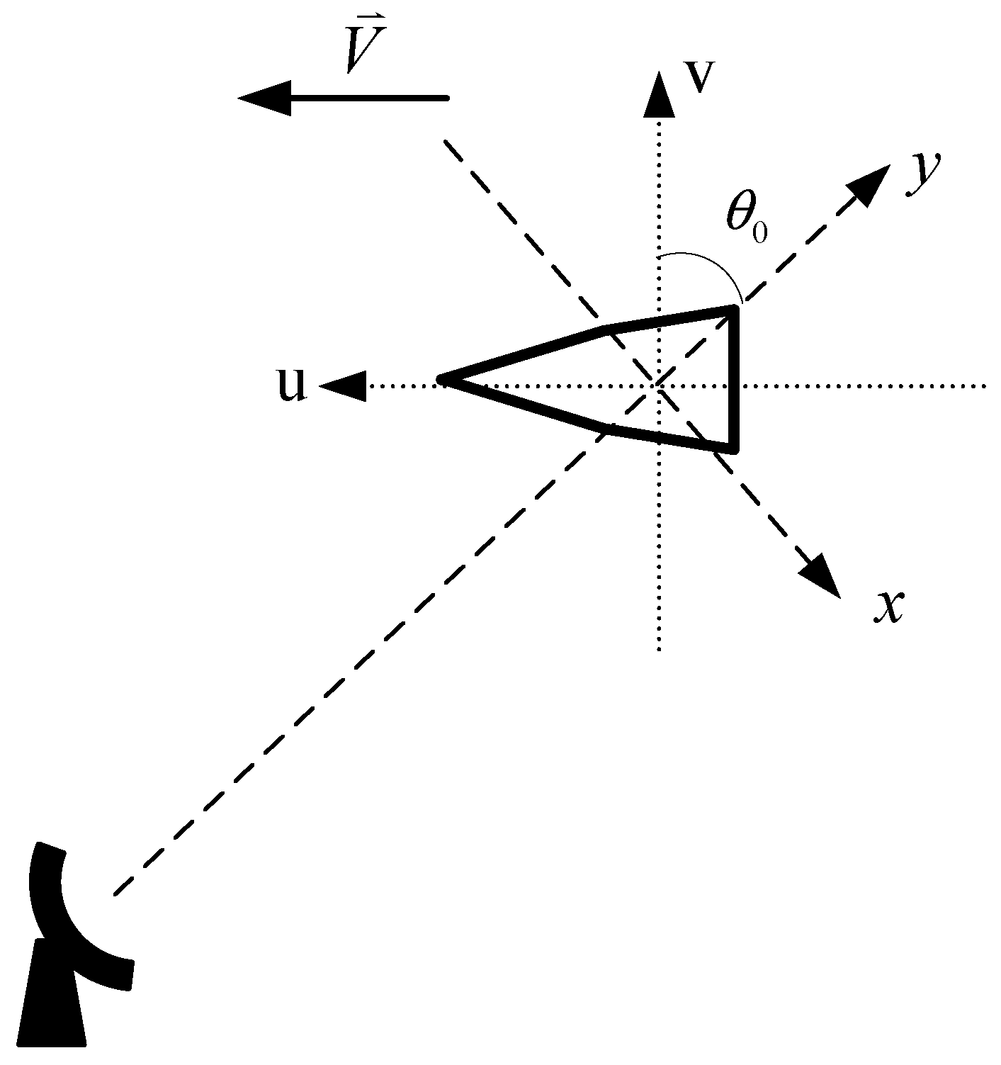
2. Radar Echo Model of Speed Compensation
3. Speed Compensation Based on CPF and ICPF
3.1. CPF
3.2. ICPF
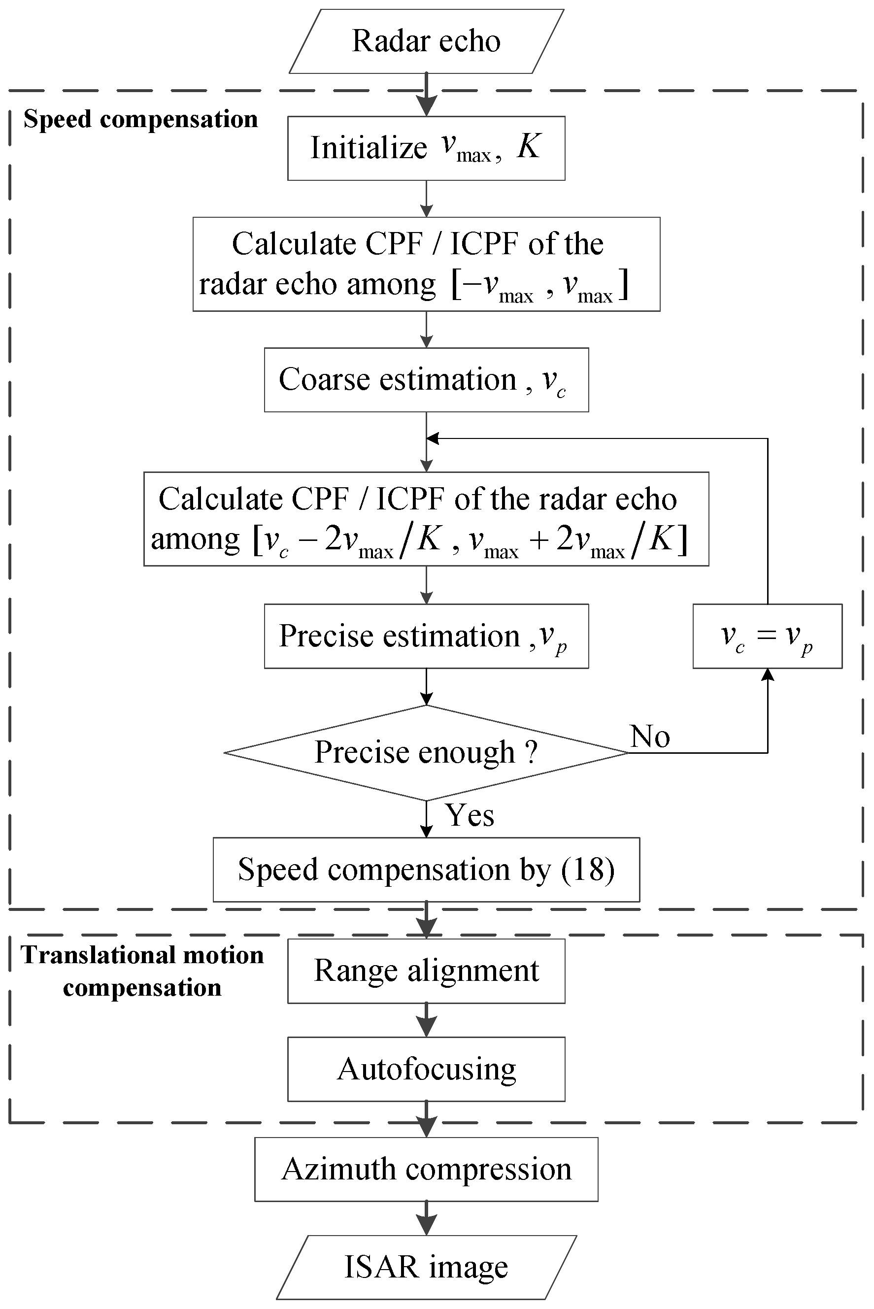
3.3. Flow Chart
- (1)
- Initialize the bound and sample number of the search of speed, which are represented as and K, respectively;
- (2)
- Calculate CPF or ICPF of the de-chirped radar echo, where the bound of the frequency axis of CPF or ICPF is determined by . The relationship between is shown as follows:
- (3)
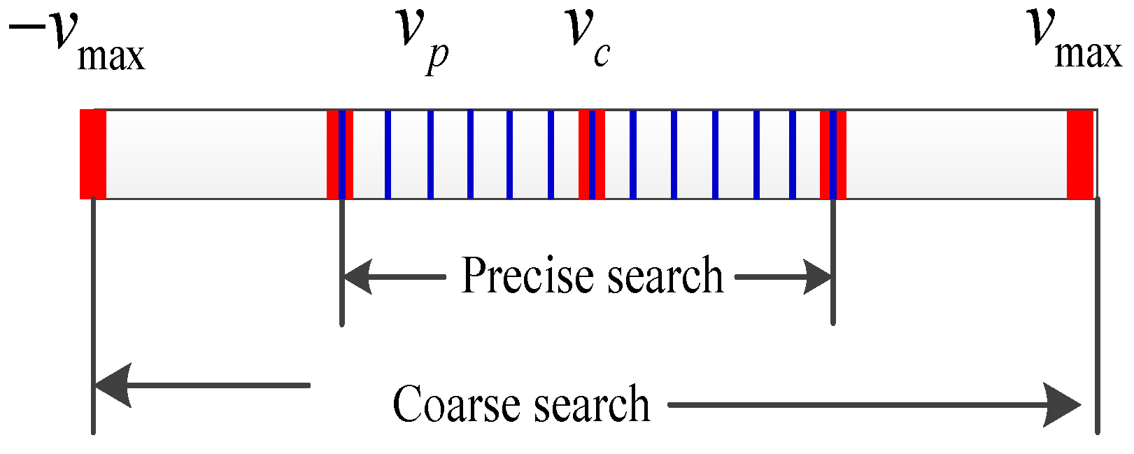
- Search CPF or ICPF to obtain the coarse estimation of speed by Equation (17) or Equation (22). The precision of the coarse estimation of speed is .
- (4)
- Reduce the bound of the search to , so as to obtain more precise estimation of speed.
- (5)
- Search CPF or ICPF to obtain the precise estimation of the speed by Equation (17) or Equation (22).
- (6)
- Judge whether the estimation of speed reaches the expected precision. If it does, compensate the speed by Equation (18) or turn to Step Equation (4) to repeat the precise estimation.


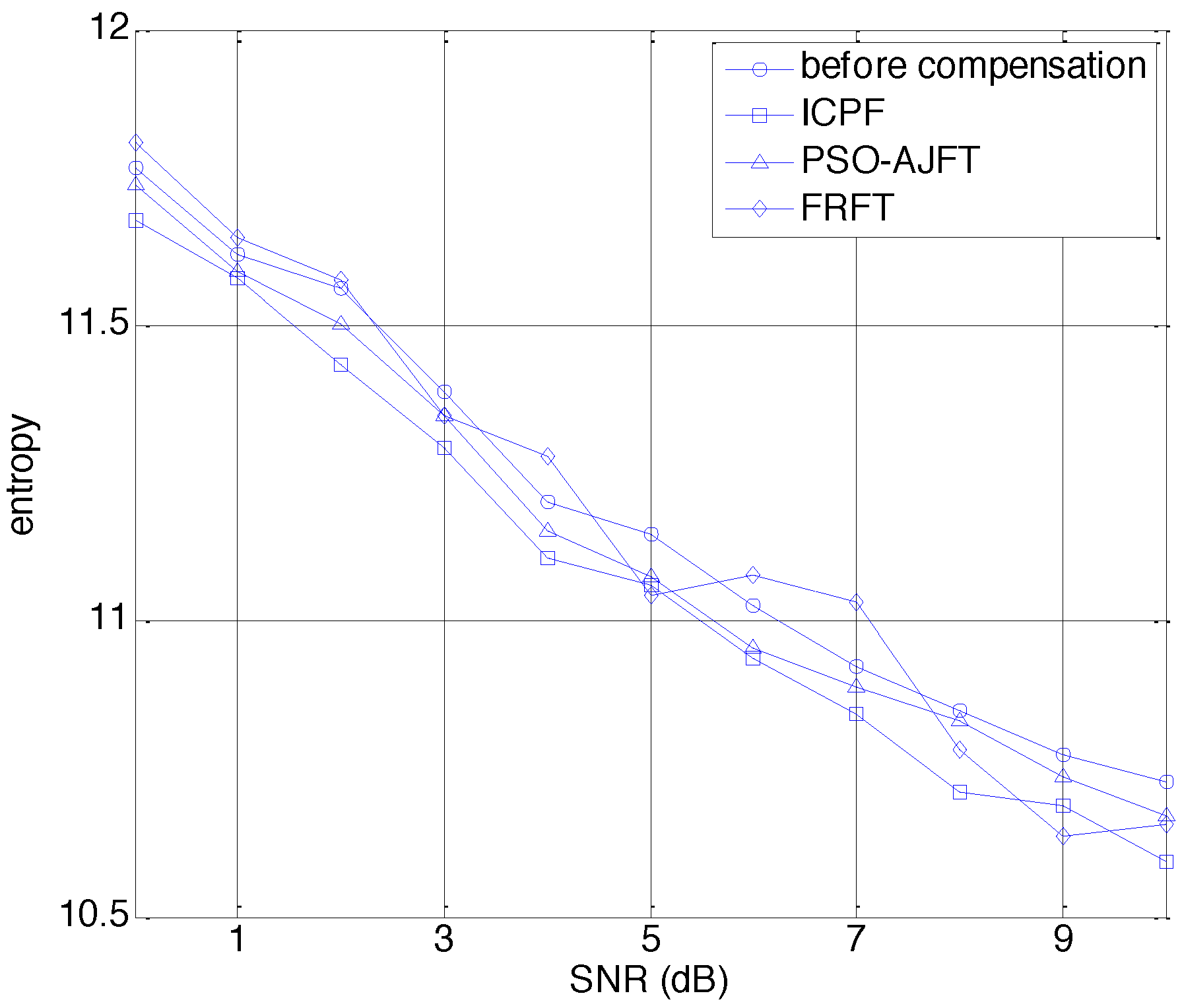
4. Experiments
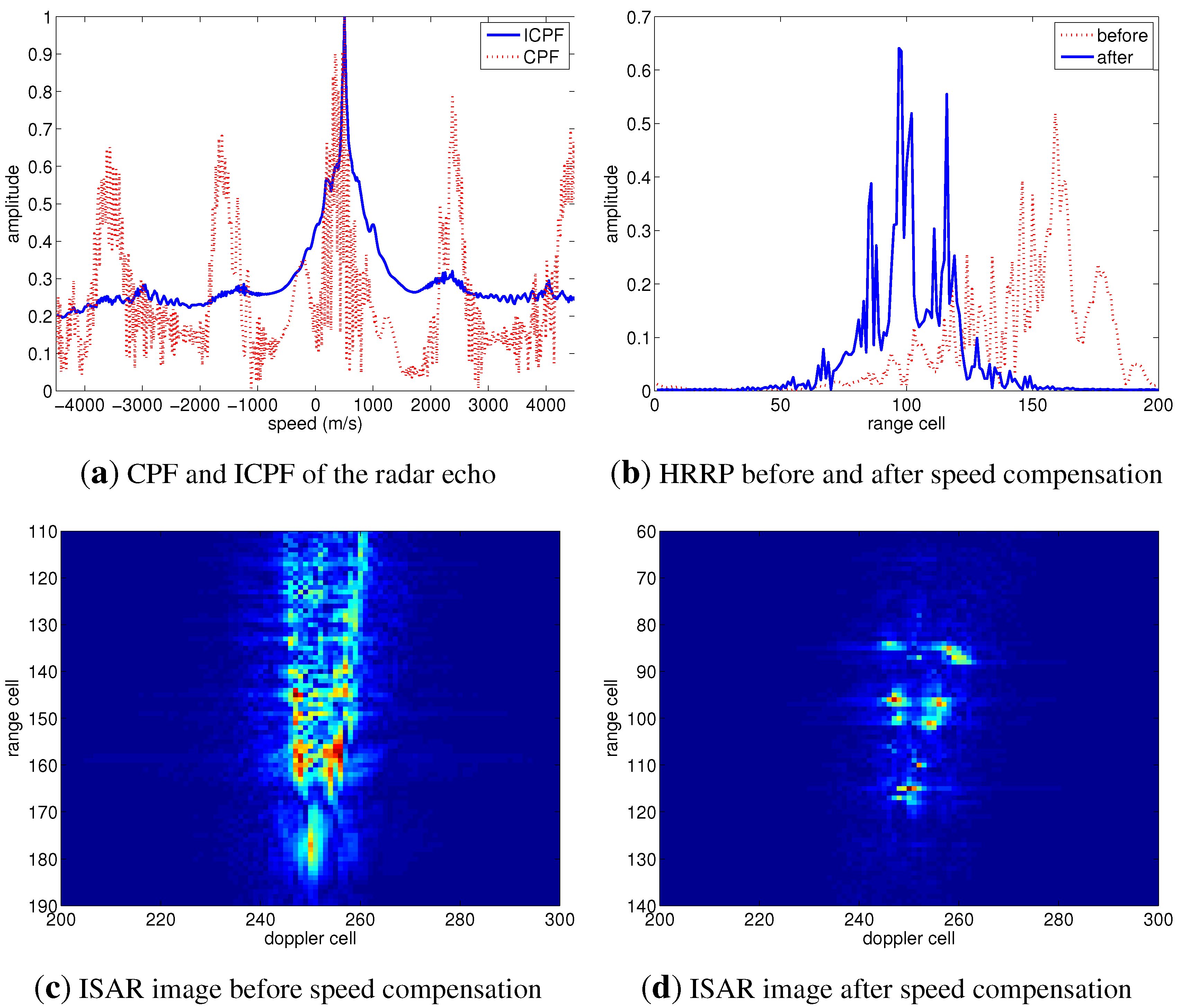
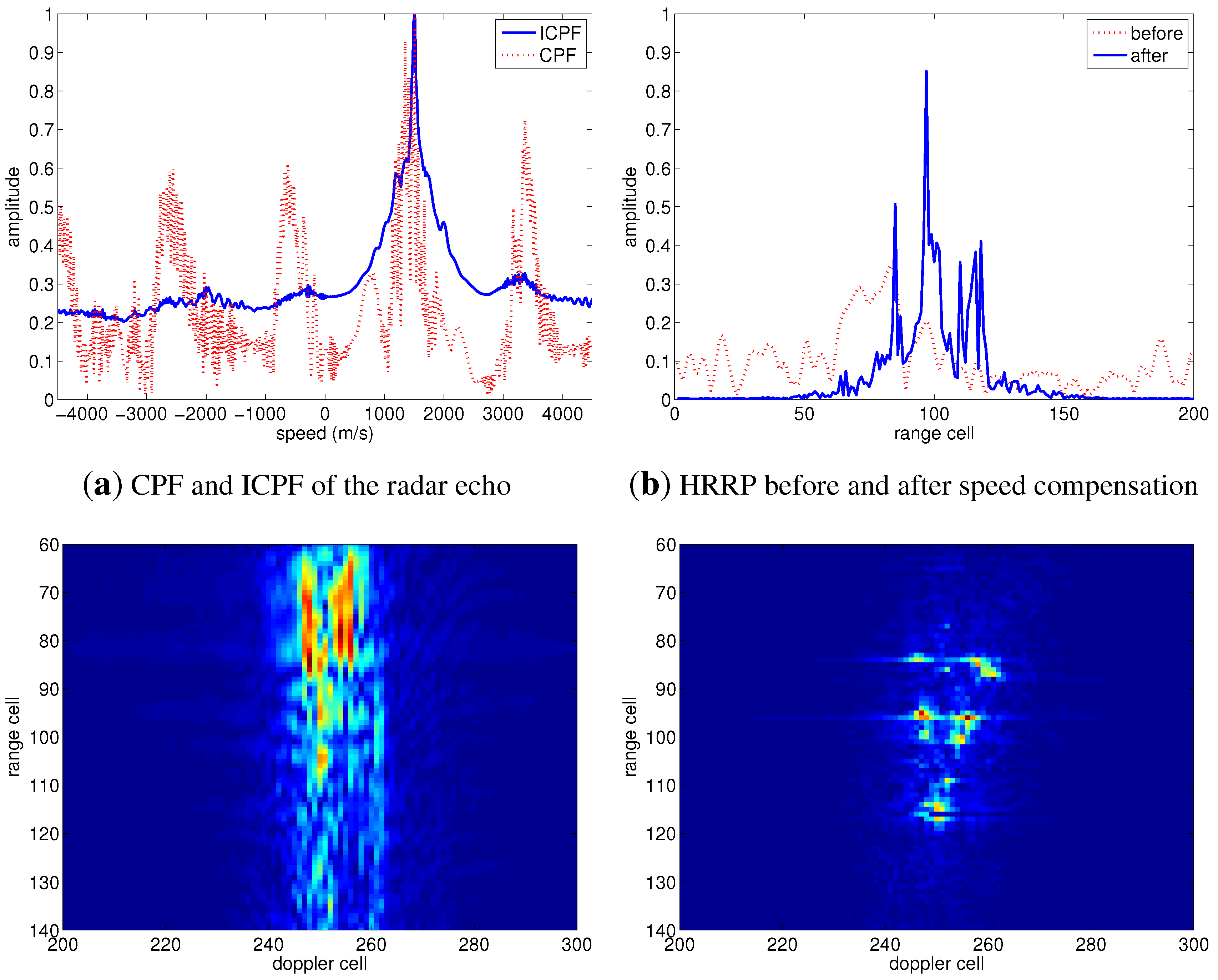
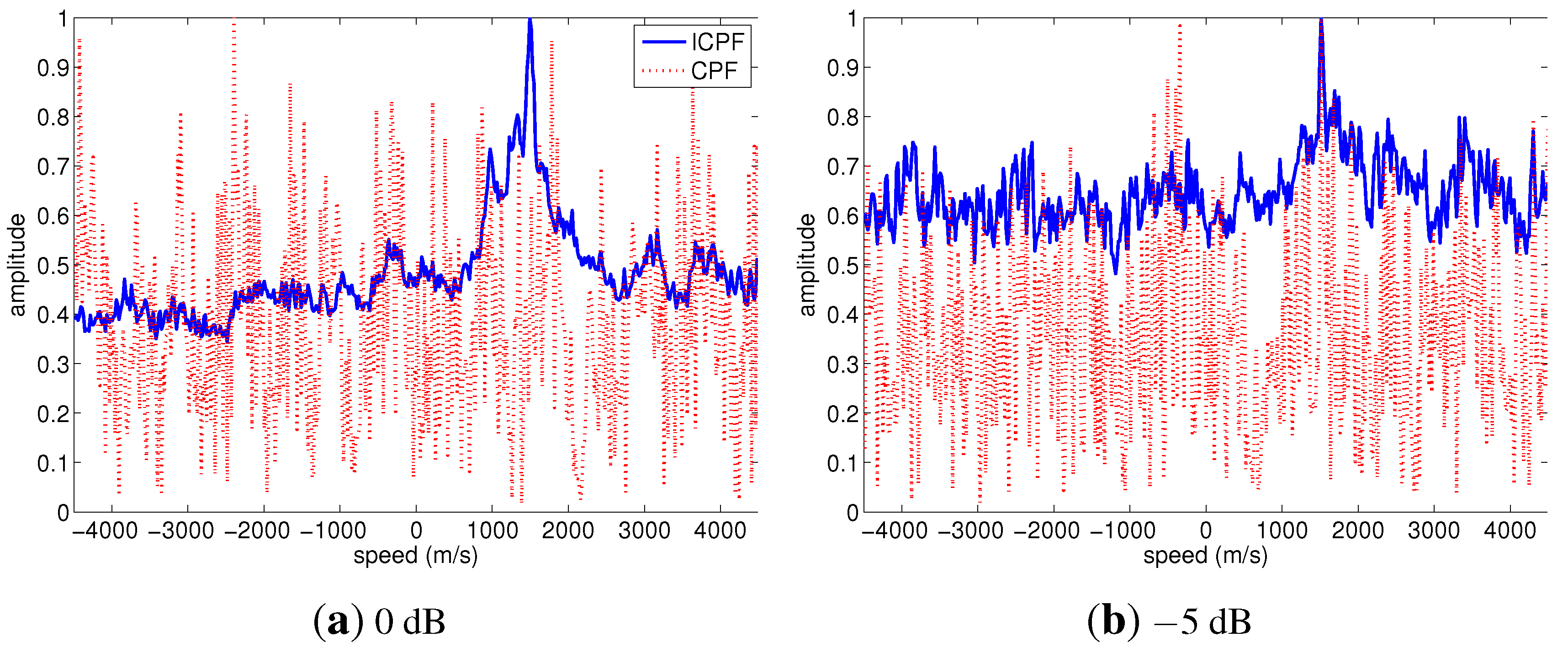
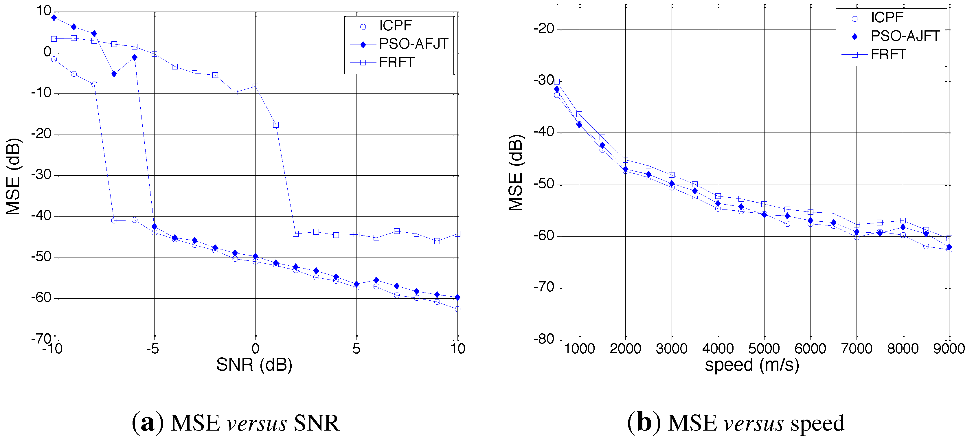
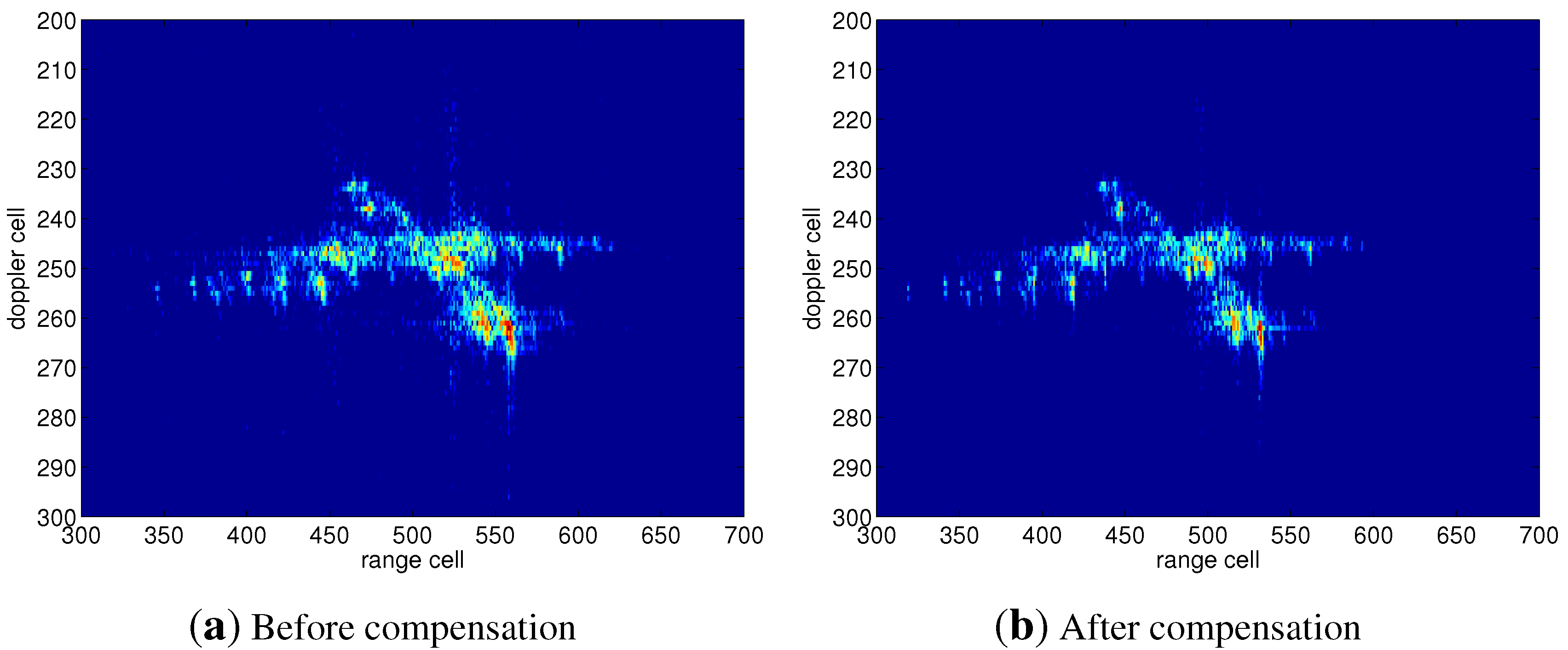
4.1. Experiment Based on the Data of a Cone-Shaped Model


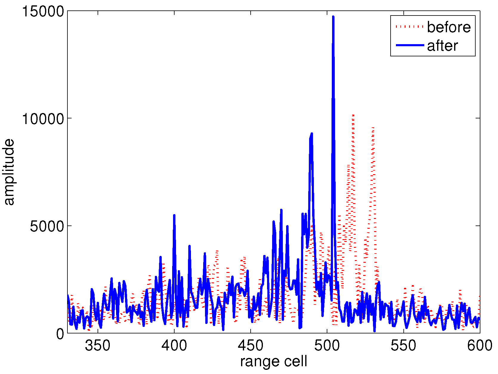
4.2. Experiment Based on the Radar Data of an Aircraft


5. Conclusions
Acknowledgments
Author Contributions
Conflicts of Interest
References
- Cuomo, K.M.; Piou, J.E.; Mayhan, J.T. Ultra-wideband coherent processing. Linc. Lab. J. 1997, 10, 203–222. [Google Scholar]
- Sadjadi, F.A. New experiments in inverse synthetic aperture radar image exploitation for maritime surveillance. In proceedings of the SPIE 9090, Automatic Target Recognition XXIV, Baltimore, MD, USA, 13 June 2014.
- Sadjadi, F. New comparative experiments in range migration mitigation methods using polarimetric inverse synthetic aperture radar signatures of small boats. In proceedings of the 2014 IEEE, Radar Conference, Cincinnati, OH, USA, 19–23 May 2014; pp. 0613–0616.
- Huang, X.; Qiu, Z.; Wei, W. Research on effect of wideband range profile imaging and compensating method for target moving with high velocity. Signal Process. 2002, 18, 487–490. [Google Scholar]
- Liu, A.F.; Zhu, X.H.; Liu, Z. ISAR range profile compensation of fast-moving target using modified discrete Chirp-Fourier transform. Acta Aeronaut. Astronaut. Sin. 2004, 25, 495–498. [Google Scholar]
- Liu, A.; Zhu, X.; Lu, J.; Liu, Z. Inverse synthetic aperture radar range profile compensation of fast-moving targets using discrete match Fourier transform. Acta Armamentarii 2004, 25, 782–785. [Google Scholar]
- Gao, X.; Ren, S.; Li, X.; Zhuang, Z. Motion compensation of a space target based on mc-PPS model. Syst. Eng. Electron. 2004, 9, 13. [Google Scholar]
- Brinkman, W.; Thayaparan, T. Focusing ISAR images using the AJTF optimized with the GA and the PSO algorithm-comparison and results. In Proceedings of the 2006 IEEE Conference on Radar, New York, NY, USA, 24–27 April 2006.
- Cao, M.; Fu, Y.; Jiang, W.; Li, X.; Zhuang, Z. High resolution range profile imaging of high speed moving targets based on fractional Fourier transform. In Proceedings of the SPIE 6786, MIPPR 2007: Automatic Target Recognition and Image Analysis; and Multispectral Image Acquisition, Wuhan, China, 15 November 2007; pp. 678654–678654.
- O’shea, P. A new technique for instantaneous frequency rate estimation. IEEE Signal Process. Lett. 2002, 9, 251–252. [Google Scholar] [CrossRef] [Green Version]
- O’Shea, P. A fast algorithm for estimating the parameters of a quadratic FM signal. IEEE Trans. Signal Process. 2004, 52, 385–393. [Google Scholar] [CrossRef] [Green Version]
- Wang, P.; Li, H.; Djurovic, I.; Himed, B. Integrated cubic phase function for linear FM signal analysis. IEEE Trans. Aerosp. Electron. Syst. 2010, 46, 963–977. [Google Scholar] [CrossRef]
- Bao, Z.; Xing, M.; Wang, T. Radar Imaging Technology; Publishing House of Electronics Industry: Beijing, China, 2005; pp. 125–129. [Google Scholar]
- Wang, J.; Liu, X.; Zhou, Z. Minimum-entropy phase adjustment for ISAR. IEE Proc. Radar Sonar Navig. 2004, 151, 203–209. [Google Scholar] [CrossRef]
© 2015 by the authors; licensee MDPI, Basel, Switzerland. This article is an open access article distributed under the terms and conditions of the Creative Commons Attribution license (http://creativecommons.org/licenses/by/4.0/).
Share and Cite
Liu, Y.; Zhang, S.; Zhu, D.; Li, X. A Novel Speed Compensation Method for ISAR Imaging with Low SNR. Sensors 2015, 15, 18402-18415. https://doi.org/10.3390/s150818402
Liu Y, Zhang S, Zhu D, Li X. A Novel Speed Compensation Method for ISAR Imaging with Low SNR. Sensors. 2015; 15(8):18402-18415. https://doi.org/10.3390/s150818402
Chicago/Turabian StyleLiu, Yongxiang, Shuanghui Zhang, Dekang Zhu, and Xiang Li. 2015. "A Novel Speed Compensation Method for ISAR Imaging with Low SNR" Sensors 15, no. 8: 18402-18415. https://doi.org/10.3390/s150818402