Creating Diversified Response Profiles from a Single Quenchometric Sensor Element by Using Phase-Resolved Luminescence

Abstract

We report a new strategy for generating a continuum of response profiles from a single luminescence-based sensor element by using phase-resolved detection. This strategy yields reliable responses that depend in a predictable manner on changes in the luminescent reporter lifetime in the presence of the target analyte, the excitation modulation frequency, and the detector (lock-in amplifier) phase angle. In the traditional steady-state mode, the sensor that we evaluate exhibits a linear, positive going response to changes in the target analyte concentration. Under phase-resolved conditions the analyte-dependent response profiles: (i) can become highly non-linear; (ii) yield negative going responses; (iii) can be biphasic; and (iv) can exhibit super sensitivity (e.g., sensitivities up to 300 fold greater in comparison to steady-state conditions).

1. Introduction

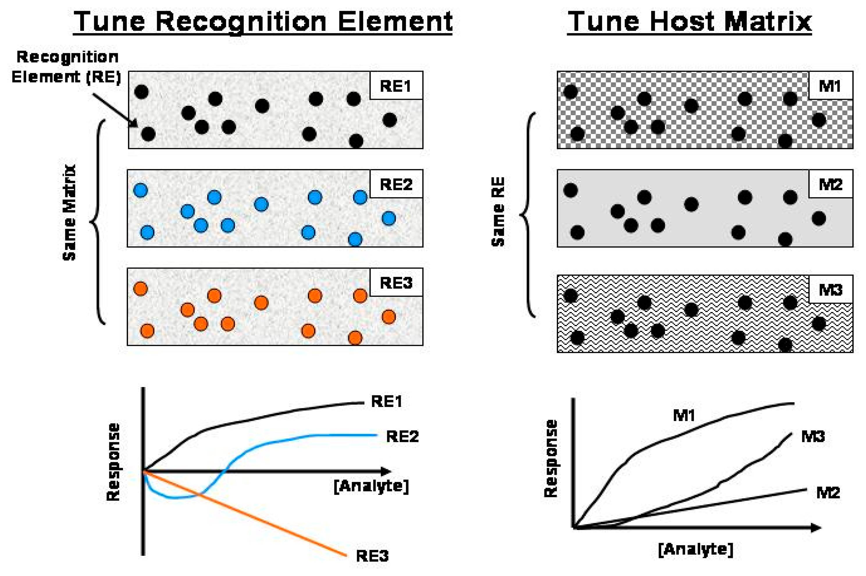
There has been significant effort devoted to creating optical chemical sensors for a wide variety of target analytes [1–5]. There have also been simultaneous and largely related efforts to create ensembles of sensors that act independently and provide unique responses for the same target analyte (i.e., diversified responses; 1 analyte, n sensor elements, n ≫ 1)) and this concept has also been extended to simultaneous multi-analyte detection (m analytes, n sensor elements; n ≫ m) [3,6–11]. In all previous efforts, researchers have created sensor ensembles and thus diversified responses by adjusting the: (a) individual recognition elements within the analyte-permeable host matrix and/or (b) host matrix to control the partitioning of the target analyte into the host matrix and eventual interaction with the recognition element, as illustrated in Figure 1 [12–14].

In this paper, we describe a strategy for creating a continuously tunable response from a single sensor element. The approach exploits a unique feature of phase-resolved luminescence [15]. The potential of this strategy is demonstrated for a single O₂-responsive xerogel-based sensor element as it offers a simple and well understood behavior. Consider the following scenario: (i) a single type of luminophore molecule sequestered within a quencher-permeable host matrix; (ii) these luminophore molecules emit from largely similar microenvironments; and (iii) the quencher molecules have similar accessibilities to the individual luminophore molecules. Under steady-state illumination conditions, one can write the Stern-Volmer relationship [16] given by Equation (1):

$$I_0/I=1+K_{\text{SV}}[\text{Q}]$$

(1)

where in this expression, [Q] is the concentration of quencher, I₀ and I represent the steady-state luminescence intensities in the absence and presence of quencher, Q, respectively, and K_SV is the Stern-Volmer quenching constant. Under dynamic quenching conditions, K_SV depends on k_Q, the bimolecular quenching constant that describes the luminophore and quencher interaction and τ₀, the luminophore excited-state luminescence lifetime in the absence of any quencher molecules (i.e., K_SV = k_Q τ₀) [16].

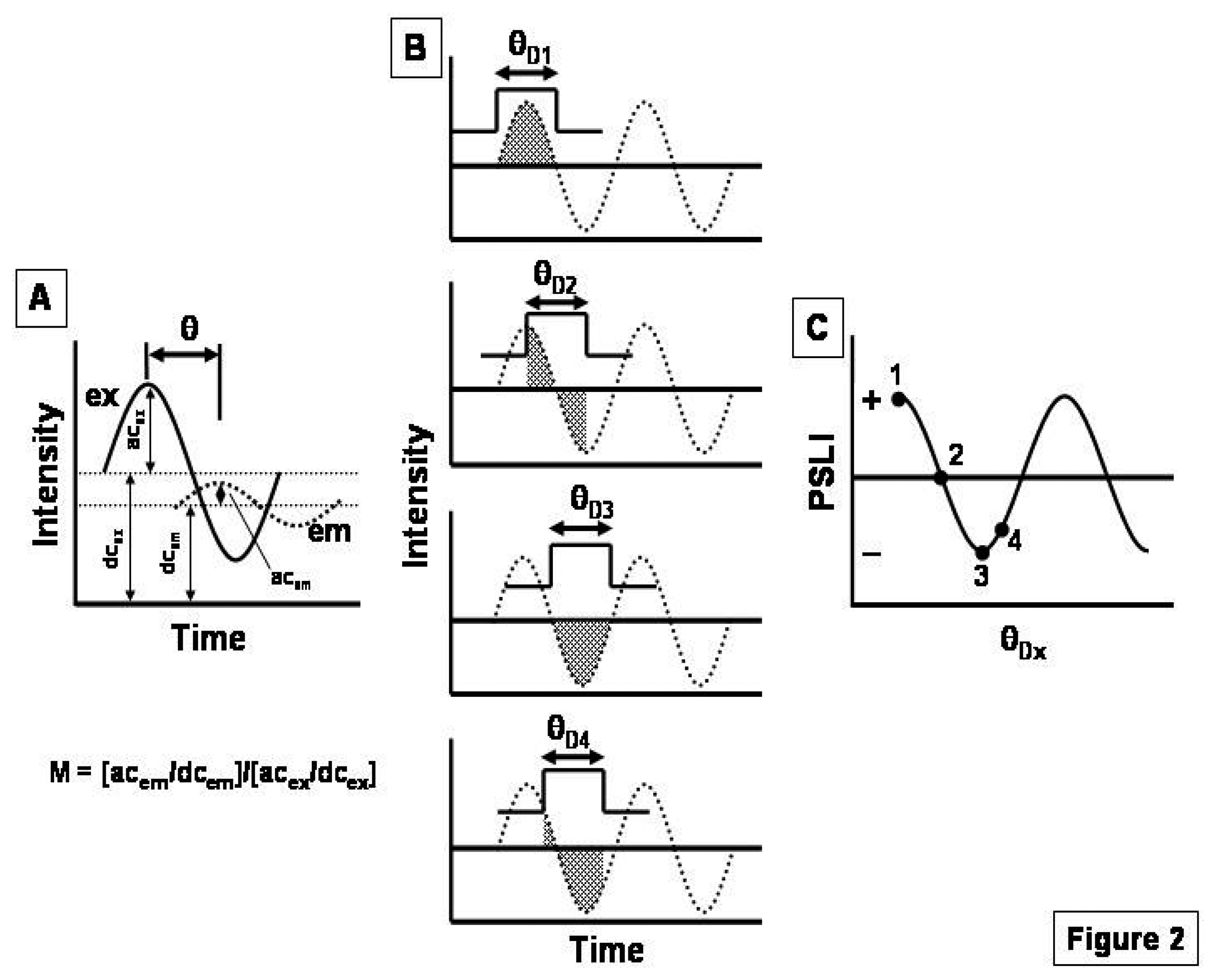
If we electronically excite (ex) the luminophores within this same sensor element by using sinusoidally modulated electromagnetic radiation (Figure 2A) at frequency (f), the resulting emission (em) will be phase shifted (θ) and demodulated (M) in comparison to the excitation by an extent that depends on the luminophore excited-state lifetime (τ) [17,18]:

$$\theta =arctan(2\pi f\tau )$$

(2)

$$M={\left[1+{\left(2\pi f\right)}^2{\tau }^2\right]}^{-1/2}$$

(3)

In turn, we can write expressions for I and τ at any Q concentration as:

$$I=I_0/[1+(k_{\text{Q}}{\tau }_0[\text{Q}])]$$

(4)

$$\tau =1/[1/{\tau }_0+k_{\text{Q}}[\text{Q}]]$$

(5)

If we record the luminescence from this same sensor element using a phase-sensitive detector (i.e., a lock-in amplifier) (Figure 2B,C) [15], we can write an expression for the phase-sensitive luminescence intensity (PSLI) as Equation (6):

$$\text{PSLI}({\theta }_{\text{D}})=IMcos({\theta }_{\text{D}}-\theta )$$

(6)

where I denotes the steady-state luminescence intensity, M represents the demodulation factor, θ_D is the detector (i.e., lock-in amplifier) phase angle, and θ is the luminescence phase angle (all terms depend on Q). If we substitute Equations (2)–(5) into Equation (6), we can write an expression for the phase-sensitive analog of Equation (1), namely as:

$${\text{PSLI}}_0/\text{PSLI}=\left[I_0{M}_{0}cos({\theta }_{\text{D}}-{\theta }_0)\right]/\left[IMcos({\theta }_{\text{D}}-\theta )\right]$$

(7)

Equation (7) provides the key relationship between the fundamental properties of the sensor element (i.e., k_Q, τ₀, and I₀) and the phase-sensitive analog of I₀/I (i.e., PSLI₀/PSLS) as a function of [Q], θ_D, and f. Inspection of Equation (7), suggests a strategy for tuning the response profiles (i.e., creating diversity) from a single sensor element by adjusting θ_D and f.

2. Experimental Section

2.1. Chemical Reagents

Tris(4,7′-diphenyl-1,10′-phenanathroline) ruthenium(II) chloride pentahydrate ([Ru(dpp)₃]²⁺) was purchased from GFS Chemicals, Inc. (Powell, OH, USA) and purified as described in the literature [19]. Tetraethyorthosilane (TEOS) and n-octyltriethoxysilane (C8-TEOS) were purchased from Gelest, Inc. (Morrisville, PA, USA). HCl was obtained from Fisher Scientific Co. (Pittsburgh, PA, USA). EtOH was a product of Quantum Chemical Corp. (New York, NY, USA). Deionized water was prepared to a specific resistivity of at least 18 MΩ-cm by using a Barnstead NANOpure^® II system.

2.2. Preparation of [Ru(dpp)₃]²⁺-Doped Xerogel Sensing Films

The sol solutions were prepared as described elsewhere [20]. Xerogel films were formed directly onto the surface of a light emitting diode (LED, λ_max = 468 nm, Stanley Electric Co., Inc., (Tokyo, Japan). The LED surface was cleaned first by rinsing with 1 M NaOH then with copious amounts of deionized water and EtOH, and allowed to dry under ambient conditions. Films were formed by depositing 20 μL of sol solution on to the LED surface. Xerogel-coated LEDs were stored in the dark under ambient conditions for at least seven days before evaluation. Previous research [20] has shown that these class II xerogel-based sensor elements exhibit linear I₀/I vs. O₂ plots and the responses are stable for several years.

2.3. Instrumentation

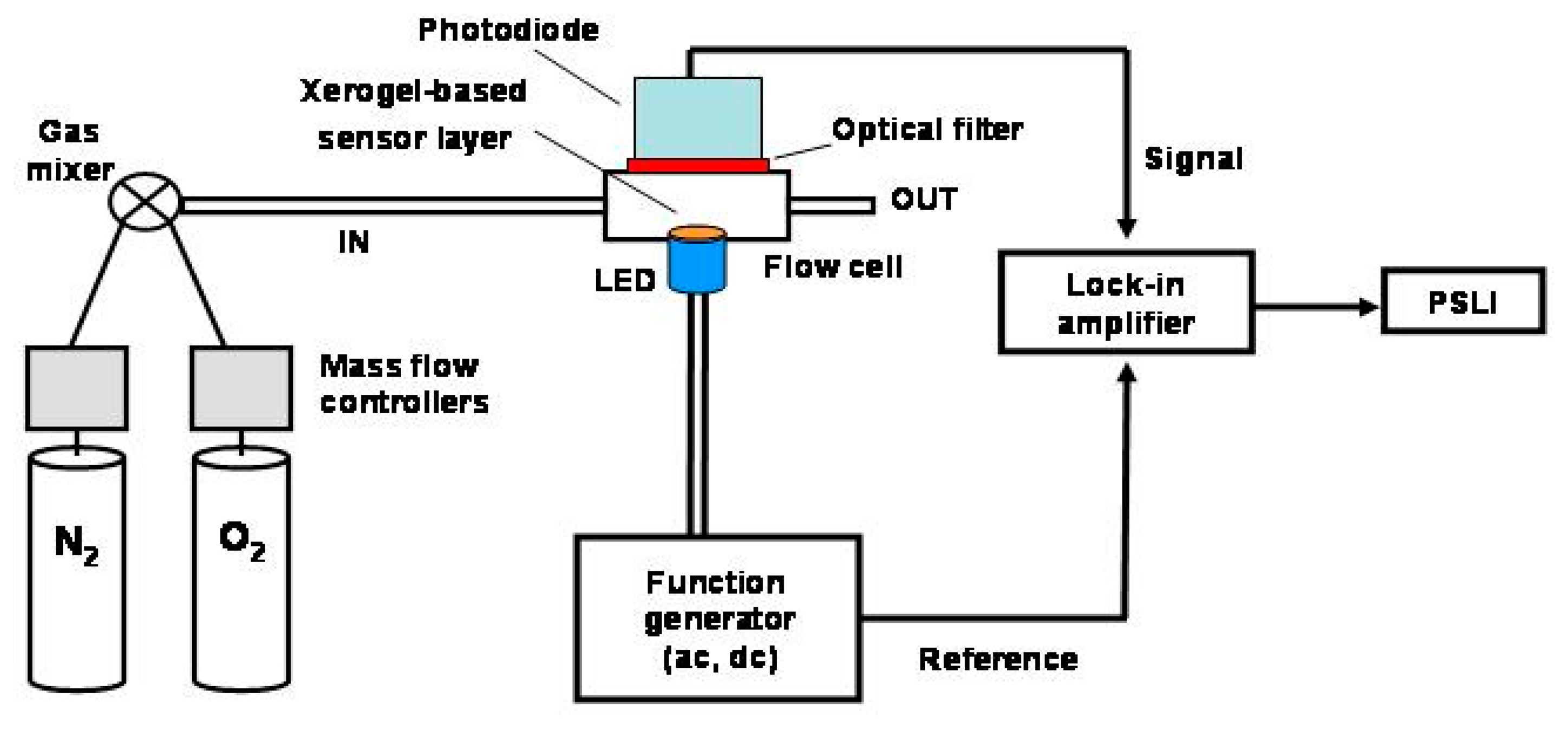
Figure 3 presents a simplified schematic of the phase-resolved luminescence system that was constructed for this research. A model DS345 function generator (Stanford Research Systems, Sunnyvale, CA, USA) provided the AC and DC components to drive the LED. The function generator output also served as the reference input to a Stanford Research Systems (model SR830) lock-in amplifier. The xerogel-coated LED was enclosed within an optically transparent housing with an inlet/outlet for gas flow. In the current experiments, the quencher was gaseous O₂. The emission was monitored through a 570 nm long pass optical filter (Oriel, Irvine, CA, USA) and detected by a 1 MHz bandwidth silicon photodiode (Thorlabs, Inc., Newton, NJ, USA). The photodiode output signal was directed to the lock-in amplifier input. The lock-in amplifier served to record the phase sensitive luminescence intensity (PSLI) at a given detector phase angle setting (θ_D).

In a typical experiment, we adjust the excitation modulation frequency (f) to a given value (20 or 50 kHz) and increment θ_D in 22.5° steps from 0° to 180°. We then systematically adjust the environment surrounding the sensor from pure N₂ to pure O₂ by using a pair of precision mass flow controllers (model PC1NP1U1V_1A, Sensirion Inc. (Westlake Village, CA, USA). Equilibrium is evident when the luminescence intensity remains constant to within ±2%. There was no detectable sensor response hysteresis or photo-bleaching. The O₂ concentrations were accurate to ±0.8% between 10% and 100% full scale and to ±0.08% below 10% full scale.

The θ_D-, f-, and O₂-dependent phase-resolved Stern-Volmer plots were then constructed. Sensors were prepared in triplicate and replicates were prepared using at least three reagent batches on different days. All experiments were performed in at least triplicate over the course of several months. Results are reported as the mean for all measurements under a given set of conditions ± one standard deviation.

3. Results and Discussion

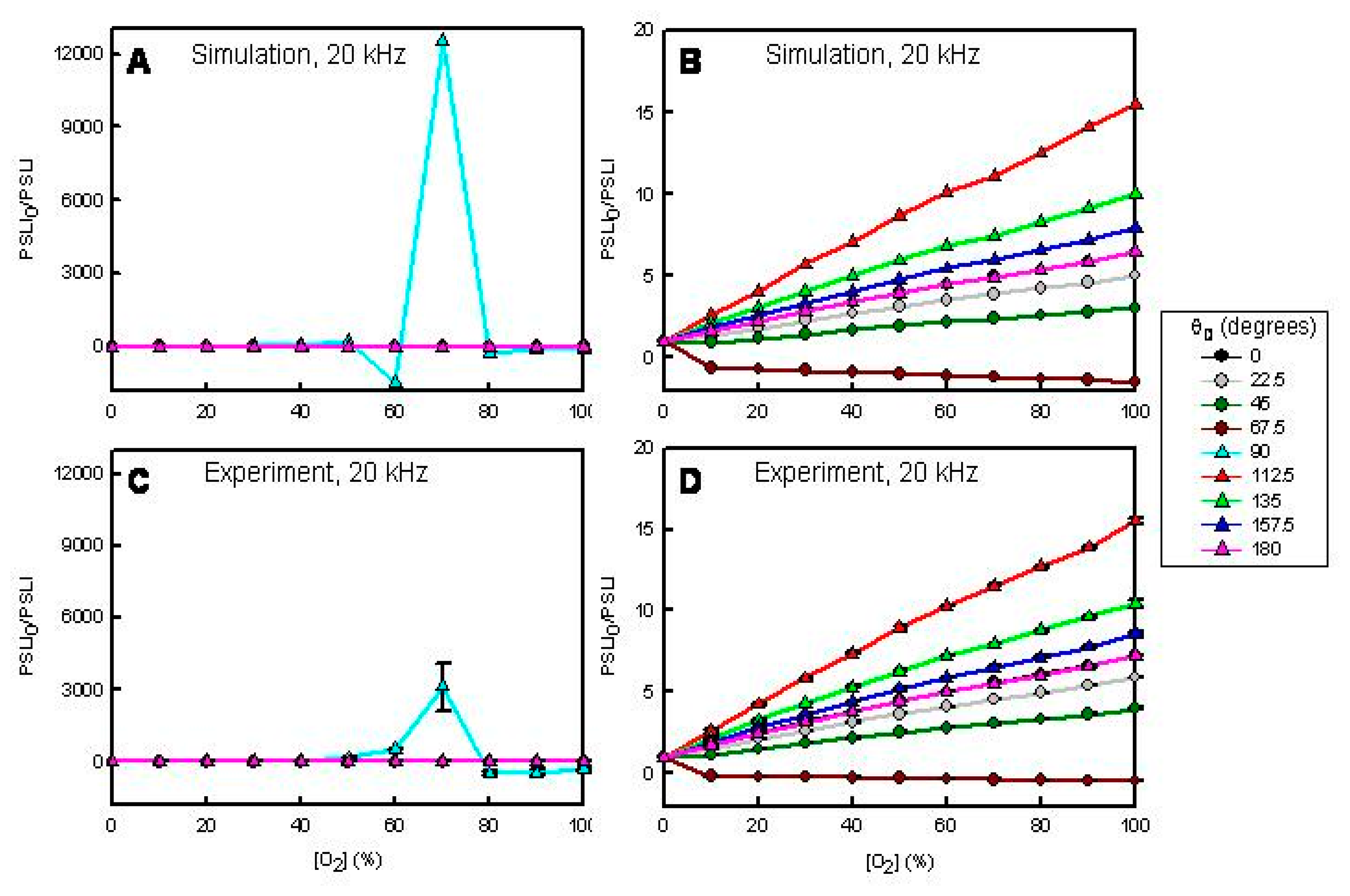
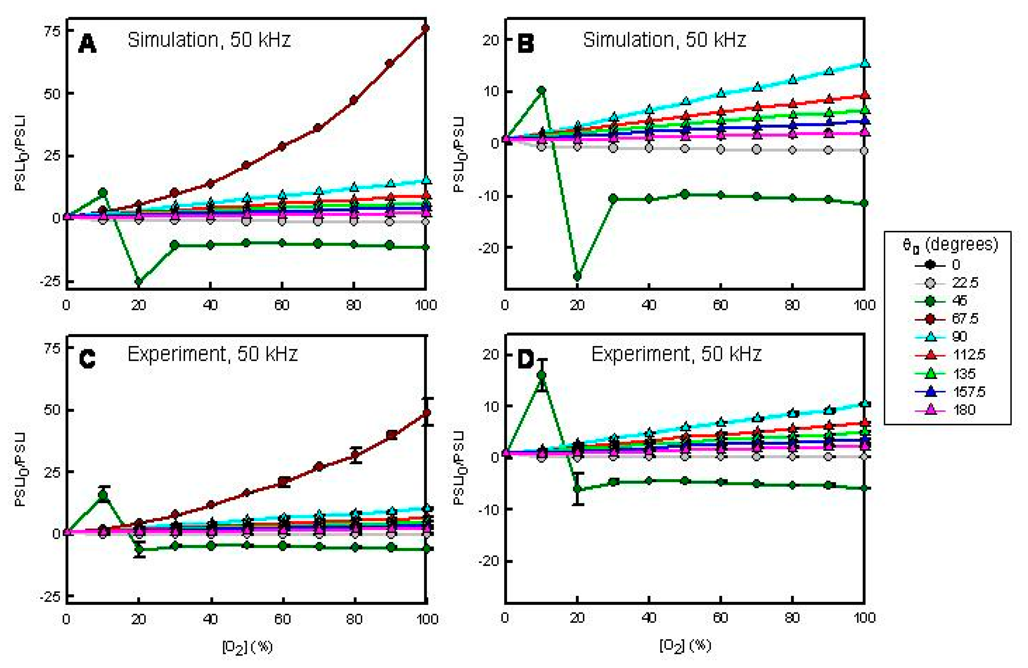
Figures 4 and 5 present simulated (A and B) and experimental (C and D) results for the sensor film when modulated at 20 and 50 kHz, respectively, as a function of O₂ (quencher) concentration and θ_D. In the simulations we assumed: τ₀ = 5.0 μs and K_SV = 0.1 O₂%⁻¹. Figures 4A and 5A show the simulated responses at each θ_D. Figures 4B and 5B show the simulated response with the highest responses (θ_D = 90° in Figure 4A, θ_D = 67.5° in Figure 5A) removed. Figures 4C and 5C show the experimental responses at each θ_D. Figures 4D and 5D show the experimental responses with the highest responses (θ_D = 90° in Figure 4C, θ_D = 67.5° in Figure 5C) removed.

Inspection of these data sets shows several interesting results. First, the simulations and experiments agree very well. Second, the response profiles depend on f and θ_D. Thus, one can tune the sensor response and sensitivity simply by adjusting f or θ_D. In all previous sensor research, there was no provision for achieving a diverse response from a single sensor element (cf., Figure 1). Third, the response profiles are sometimes non-linear. In a steady-state experiment this sensor element exhibits a linear response with a K_SV of ∼0.1 O₂%⁻¹ [20]. Fourth, there are conditions when the phase-resolved Stern-Volmer plots exhibit negative going responses due to negative phase shift change. Fifth, there are conditions when the phase-resolved Stern-Volmer plots exhibit biphasic response profiles. Finally, there are conditions when the response (PSLI₀/PSLI) is ultra-sensitive. For example, in our previous work, the I₀/I for 70% O₂ is ∼8 for this sensor element [20]. In Figure 4C we show a reproducible response in excess of 3000 at 20 kHz with a θ_D of 90°. Similarly, at 50 kHz with a θ_D of 67.5° we see a PSLI₀/PSLI at 100% O₂ of ∼50 whereas the I₀/I at 100% O₂ is ∼10 for this same sensor [20].

4. Conclusions

We report on a simple and new approach for creating diversified sensor responses from a single sensor element. The approach is not only limited to quenchometric-based sensing, but also will work under any situation where there is a change in a luminophore excited state lifetime caused by the target analyte [21–25]. Phase-sensitive detection also leads to unique analyte-dependent response profiles that are not realized under previously used detection formats. These diversified responses are ideal for training artificial neural networks (ANNs) to identify patterns and features for improving the accuracy and precision of analyte concentration determinations [26]. This strategy of creating a diversified response from a single sensor element could also enable novel miniaturized sensor systems with built-in self-testing when integrated with a tunable multi-frequency phase fluorometric spectroscopic systems [27].

References

- Narayanaswamy, R.; Wolfbeis, O.S. Optical Sensors: Industrial, Environmental and Diagnostic Applications; Springer: Berlin, Germany, 2004. [Google Scholar]
- Wang, X.D.; Wolfbeis, O.S. Optical methods for sensing and imaging oxygen: Materials, spectroscopies and applications. Chem. Soc. Rev. 2014, 43, 3666–3761. [Google Scholar]
- Askim, J.R.; Mahmoudi, M.; Suslick, K.S. Optical sensor arrays for chemical sensing: The optoelectronic nose. Chem. Soc. Rev. 2013, 42, 8649–8682. [Google Scholar]
- Wang, X.D.; Wolfbeis, O.S. Fiber-Optic Chemical Sensors and Biosensors (2008–2012). Anal. Chem. 2013, 85, 487–508. [Google Scholar]
- Wolfbeis, O.S.; Weidgans, B.M. Fiber optic chemical sensors and biosensors: A view back. Nato Sci. Ser. II Math. 2006, 224, 17–44. [Google Scholar]
- Wilson, M.S.; Nie, W.Y. Electrochemical multianalyte immunoassays using an array-based sensor. Anal. Chem. 2006, 78, 2507–2513. [Google Scholar]
- Heo, J.; Crooks, R.M. Microfluidic biosensor based on an array of hydrogel-entrapped enzymes. Anal. Chem. 2005, 77, 6843–6851. [Google Scholar]
- Albert, K.J.; Lewis, N.S.; Schauer, C.L.; Sotzing, G.A.; Stitzel, S.E.; Vaid, T.P.; Walt, D.R. Cross-reactive chemical sensor arrays. Chem. Rev. 2000, 100, 2595–2626. [Google Scholar]
- Diehl, K.L.; Anslyn, E.V. Array sensing using optical methods for detection of chemical and biological hazards. Chem. Soc. Rev. 2013, 42, 8596–8611. [Google Scholar]
- Rakow, N.A.; Suslick, K.S. A colorimetric sensor array for odour visualization. Nature 2000, 406, 710–713. [Google Scholar]
- Nagl, S.; Wolfbeis, O.S. Optical multiple chemical sensing: Status and current challenges. Analyst 2007, 132, 507–511. [Google Scholar]
- Chodavarapu, V.P.; Bukowski, R.M.; Kim, S.J.; Titus, A.H.; Cartwright, A.N.; Bright, F.V. Multi-sensor system based on phase detection, an LED array, and luminophore-doped xerogels. Electron. Lett. 2005, 41, 1031–1033. [Google Scholar]
- Daivasagaya, D.S.; Yao, L.; Yung, K.Y.; Hajj-Hassan, M.; Cheung, M.C.; Chodavarapu, V.P.; Bright, F.V. Contact CMOS imaging of gaseous oxygen sensor array. Sens. Actuators B Chem. 2011, 157, 408–416. [Google Scholar]
- Chodavarapu, V.P.; Bukowski, R.M.; Titus, A.H.; Cartwright, A.N.; Bright, F.V. CMOS integrated luminescence oxygen multi-sensor system. Electron. Lett. 2007, 43, 688–689. [Google Scholar]
- Mcgown, L.B.; Bright, F.V. Phase-Resolved Fluorescence in Chemical-Analysis. Crit. Rev. Anal. Chem. 1987, 18, 245–298. [Google Scholar]
- Lakowicz, J.R. Principle of Fluorescence Spectroscopy: Second Edition; Kluwer Academic/Plenum Publishers: New York, NY, USA, 1999. [Google Scholar]
- Gratton, E.; Jameson, D.M.; Hall, R.D. Multifrequency Phase and Modulation Fluorometry. Annu. Rev. Biophys. Bioeng. 1984, 13, 105–124. [Google Scholar]
- Jameson, D.M.; Gratton, E.; Hall, R.D. The Measurement and Analysis of Heterogeneous Emissions by Multifrequency Phase and Modulation Fluorometry. Appl. Spectrosc. Rev. 1984, 20, 55–106. [Google Scholar]
- Lin, C.T.; Bottcher, W.; Chou, M.; Creutz, C.; Sutin, N. Mechanism of Quenching of Emission of Substituted Polypyridineruthenium(Ii) Complexes by Iron(Iii), Chromium(Iii), and Europium(Iii) Ions. J. Am. Chem. Soc. 1976, 98, 6536–6544. [Google Scholar]
- Tao, Z.Y.; Tehan, E.C.; Tang, Y.; Bright, F.V. Stable sensors with tunable sensitivities based on class II xerogels. Anal. Chem. 2006, 78, 1939–1945. [Google Scholar]
- Lakowicz, J.R. Principle of Fluorescence Spectroscopy: Third Edition; Springer: New York, NY, USA, 2006. [Google Scholar]
- McGaughey, O.; Ros-Lis, J.V.; Guckian, A.; McEvoy, A.K.; McDonagh, C.; MacCraith, B.D. Development of a fluorescence lifetime-based sol-gel humidity sensor. Anal. Chim. Acta 2006, 570, 15–20. [Google Scholar]
- Pickup, J.C.; Hussain, F.; Evans, N.D.; Rolinski, O.J.; Birch, D.J.S. Fluorescence-based glucose sensors. Biosens. Bioelectron. 2005, 20, 2555–2565. [Google Scholar]
- Collier, B.B.; McShane, M.J. Time-resolved measurements of luminescence. J. Lumin. 2013, 144, 180–190. [Google Scholar]
- Bukowski, R.M.; Chodavarapu, V.P.; Titus, A.H.; Cartwright, A.N.; Bright, F.V. Phase fluorometric glucose biosensor using oxygen as transducer and enzyme-doped xerogels. Electron. Lett. 2007, 43, 202–204. [Google Scholar]
- Tang, Y.; Tao, Z.Y.; Bukowski, R.M.; Tehan, E.C.; Karri, S.; Titus, A.H.; Bright, F.V. Tailored xerogel-based sensor arrays and artificial neural networks yield improved O2 detection accuracy and precision. Analyst 2006, 131, 1129–1136. [Google Scholar]
- Chodavarapu, V.P.; Daivasagaya, D.S. Methods and Devices for Xerogel based Sensors. U.S. Patent 2014/0080225 A1, 20 March 2014. [Google Scholar]
© 2015 by the authors; licensee MDPI, Basel, Switzerland. This article is an open access article distributed under the terms and conditions of the Creative Commons Attribution license ( http://creativecommons.org/licenses/by/4.0/).
Share and Cite
Tehan, E.C.; Bukowski, R.M.; Chodavarapu, V.P.; Titus, A.H.; Cartwright, A.N.; Bright, F.V. Creating Diversified Response Profiles from a Single Quenchometric Sensor Element by Using Phase-Resolved Luminescence. Sensors 2015, 15, 760-768. https://doi.org/10.3390/s150100760
Tehan EC, Bukowski RM, Chodavarapu VP, Titus AH, Cartwright AN, Bright FV. Creating Diversified Response Profiles from a Single Quenchometric Sensor Element by Using Phase-Resolved Luminescence. Sensors. 2015; 15(1):760-768. https://doi.org/10.3390/s150100760
Chicago/Turabian StyleTehan, Elizabeth C., Rachel M. Bukowski, Vamsy P. Chodavarapu, Albert H. Titus, Alexander N. Cartwright, and Frank V. Bright. 2015. "Creating Diversified Response Profiles from a Single Quenchometric Sensor Element by Using Phase-Resolved Luminescence" Sensors 15, no. 1: 760-768. https://doi.org/10.3390/s150100760