Evaluation of Multi-Resolution Satellite Sensors for Assessing Water Quality and Bottom Depth of Lake Garda

 , , , and
Abstract
: In this study we evaluate the capabilities of three satellite sensors for assessing water composition and bottom depth in Lake Garda, Italy. A consistent physics-based processing chain was applied to Moderate Resolution Imaging Spectroradiometer (MODIS), Landsat-8 Operational Land Imager (OLI) and RapidEye. Images gathered on 10 June 2014 were corrected for the atmospheric effects with the 6SV code. The computed remote sensing reflectance (Rrs) from MODIS and OLI were converted into water quality parameters by adopting a spectral inversion procedure based on a bio-optical model calibrated with optical properties of the lake. The same spectral inversion procedure was applied to RapidEye and to OLI data to map bottom depth. In situ measurements of Rrs and of concentrations of water quality parameters collected in five locations were used to evaluate the models. The bottom depth maps from OLI and RapidEye showed similar gradients up to 7 m (r = 0.72). The results indicate that: (1) the spatial and radiometric resolutions of OLI enabled mapping water constituents and bottom properties; (2) MODIS was appropriate for assessing water quality in the pelagic areas at a coarser spatial resolution; and (3) RapidEye had the capability to retrieve bottom depth at high spatial resolution. Future work should evaluate the performance of the three sensors in different bio-optical conditions.1. Introduction
Since the 1980s, satellite remote sensing represents an opportunity for synoptic and multi-temporal viewing of water quality of lakes [1–3]. Overall, these applications require sensors which operate in the visible-near infrared wavelengths [4], with high radiometric sensitivity [5] and a spatial/temporal resolution to adequately capture the hydrological and limnological processes in the case study. As a result, most of the work has been more accomplished with the latest generation of ocean colour sensors (i.e., MODIS and MERIS) and with Thematic Mapper (TM), an Earth observing sensor of the Landsat program. The most common methods to retrieve water quality from these sensors have been recently reviewed by Odermatt et al. [6]. They provided a comprehensive overview of water constituent retrieval algorithms in for coastal waters and lakes, including empirical approaches and physics-based bio-optical models.
The Moderate Resolution Imaging Spectroradiometer (MODIS) instrument, onboard both Terra and Aqua spacecraft (a NASA-centered international Earth Observing System), provides 12 bit imagery in 36 bands, ranging from 0.4 to 14.4 μm. MODIS is operating since 1999 (2002 for the MODIS onboard Aqua), viewing the entire surface of the Earth every one to two days. Within a viewing swath width of 2330 km, MODIS acquires data at three spatial resolutions (250 m, 500 m and 1 km). In particular, the MODIS dataset at 1 km resolution has been utilised in many studies for assessing the concentrations of water quality parameters in lakes. e.g., Chang et al., Horion et al., and Hu et al. [7–9] used MODIS to monitor phytoplankton in Lake Okeechobee (USA), in Lake Tanganyika (East African Rift) and Lake Taihu (PRC) respectively; Kaba et al., and Zhang et al. [10,11] assessed suspended particulate matter (SPM) in Lake Tana (Ethiopia) and Lake Taihu (PRC), respectively from MODIS time-series.
The Medium Resolution Imaging Spectrometer (MERIS) instrument provides 12 bit imagery, in 15 bands (from 0.4 to 1.04 μm). MERIS was part of the core instrument payload of the ESA Envisat-1 mission, which has been operating from 2002 to 2012. With a spatial resolution of 300 m, which therefore offered improved possibilities for monitoring of small to medium-sized lakes, the 10-years long record of MERIS imagery have been widely used to assess water quality in many lakes. e.g., Giardino et al., Odermatt et al., and Bresciani et al. [12–14] in the European peri-Alpine lakes; Matthews [15] in South African inland waters; Ali et al., and Binding et al. [16,17] in North America's lakes.
The longest temporal record of satellite imagery suitable for lake studies has been provided by the Landsat program. Landsat data have been acquired routinely for over 40-years: starting with Landsat 4 TM (launched in 1982) and now ongoing with the Landsat-8 Operational Land Imager (OLI), launched in 2013. Although TM shows lower radiometric sensitivity and larger bandwidths with respect to the ocean colour sensors, its spatial resolution of 30 m (combined with a revisiting time of 16 days,) made the sensor attractive for lake studies. Verpoorter et al. [18] used Landsat imagery to produce a global inventory of lakes: it contains geographic and morphometric information for ∼117 million lakes with a surface area larger than 0.01 km2. Then, water quality of lakes from Landsat has been investigated worldwide; e.g., in Asia [19,20], in Europe [21–23], in North America [24,25], in Africa [26]. Retrospective analyses with Landsat imagery were performed by Dekker et al. [27] for benthic cover change detection in a shallow tidal Australian lake and by Lobo et al. [28] for mapping the total suspended solids of the Tapajós River (Brazil) from 1973 to 2013. Pahlevan et al. [29] observed how the improved design of OLI (with respect to the previous sensors onboard of Landsat) is indeed very promising for inland water studies.
Finally, finer scale studies of aquatic remote sensing have been based on higher-spatial resolution satellite sensors (e.g., QuickBird, Ikonos, WorldWiew-2), although those sensors are known to have inferior signal to noise ratio compared to ocean colour systems [30,31] and are not completely suitable in aquatic remote sensing [32]. Their high spatial resolution (≥5 m) makes those systems very attractive in spatial heterogeneous areas. In particular, many studies [33–37] have shown how those sensors are suitable for mapping bottom properties and depth if in situ data for calibrating the algorithms are available.
In this study, we focus on Lake Garda, a large deep Italian lake characterised by clear waters and coastal areas colonised by submerged macrophyte beds. Previous remote sensing studies over Lake Garda mostly used MERIS and Landsat TM imagery to assess water composition in the lake [23,38–40], while airborne imaging spectrometry was used to assess bottom depth and benthic cover [41–43]. In all those studies, the retrieval of water components and bottom properties was achieved with physics-based models, which basically enable the correction of atmospheric effects, the conversion of the water reflectance first into inherent optical properties (IOPs) and then into concentrations of water components such as chl-a, SPM and coloured dissolved organic matter (CDOM). The in-water physics-based models were parameterized based on a long term database of ∼150 records collected from 2000 to date [23,43,44]. In case of optically shallow waters the approach also provides information on benthic substrate type and bottom depth.
In this study we evaluated the applicability of currently available satellite sensors to retrieve water composition and bottom depth in Lake Garda. The objectives in this study are: (1) to investigate the suitability of MODIS and OLI to estimate the concentrations of water components in the pelagic areas of the lake; (2) to evaluate for the first time the capability of OLI and RapidEye to retrieve the bottom depth in shallow waters. To all imagery, we applied a consistent physics-based processing chain to convert the radiances measured from satellite sensors into water reflectance, inherent optical properties, concentrations of water constituents and bottom depth according to Bresciani et al. [42] and Giardino et al. [43]. The models results were evaluated with in situ data collected during the satellite overpasses.
2. Materials and Methods
2.1. Study Area and Fieldwork Activities
Located in the Subalpine ecoregion, Lake Garda is the largest lake in Italy, having an area of 370 km2, a water volume of 50 km3 and a maximum depth of 346 m. It represents an essential strategic water supply for agriculture, industry, energy, fishing and drinking [45]. Moreover, it is an important resource for recreation and tourism with its attractions of landscape, mild climate and water quality. According to Organisation for Economic Co-operation and Development (OECD) is classified as an oligo-mesotrophic lake [46]: phosphorous concentration in the epilimnium is below or around 10 μg/L, the average concentration of chl-a is 3 mg/m3, the Secchi disk depths vary between 4–5 m in summer and 15–17 m in late winter [47]. With respect to morphology the lake can be divided in two different areas: the largest sub-basin extended from north to southwest area, characterised by deepest bottoms, and the south-eastern shallower sub-basin. The northern part of the lake is characterized by mountain slopes mainly covered by forests or rural territories, whilst the southern part of the lake is surrounded by morenic and alluvial plains and low hills with a mix of urbanised and rural land use [45].
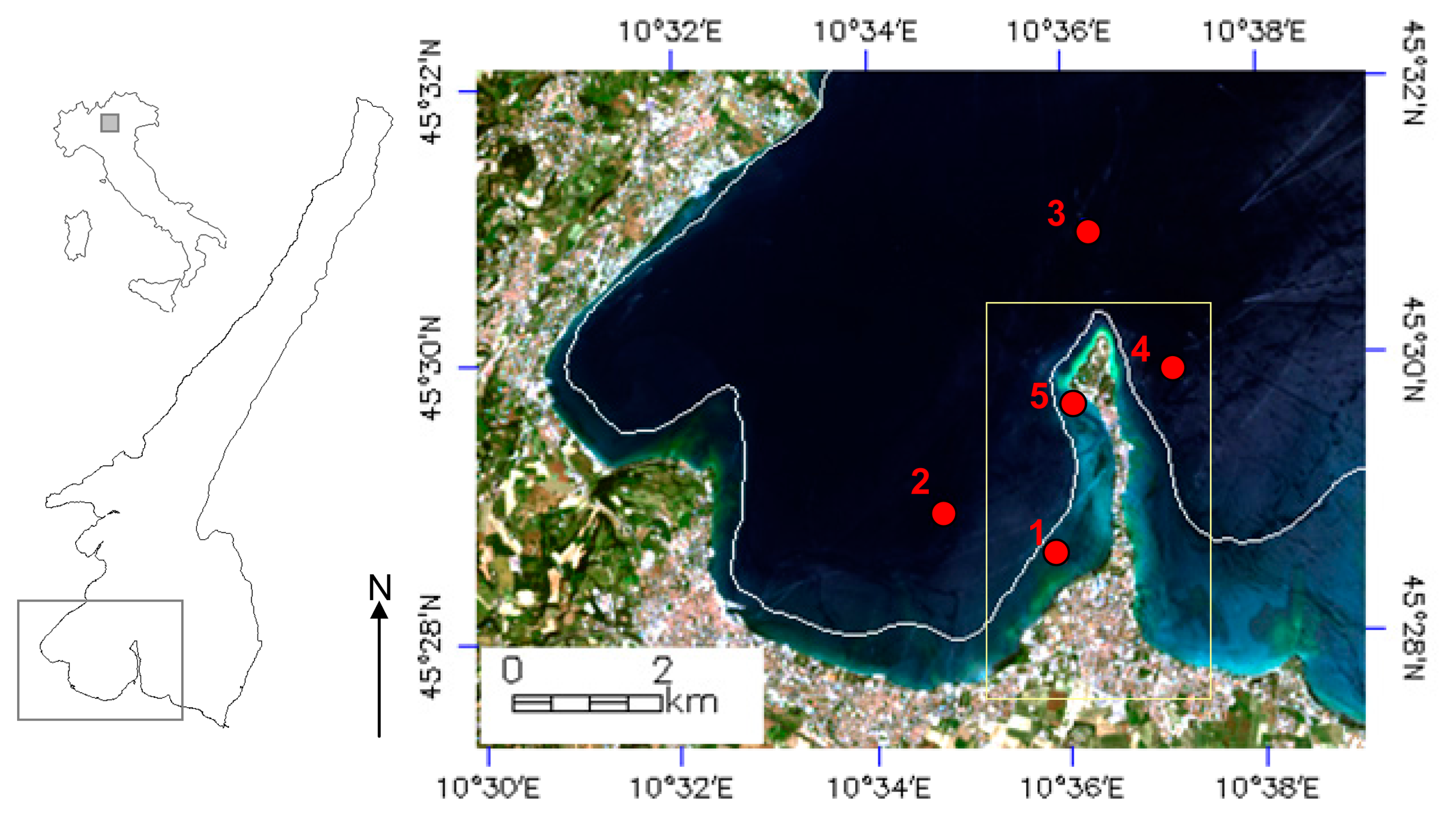
To perform an assessment of water constituents and bottom retrievals from multi-resolution satellite sensors with the use of match-ups with in situ data, a field campaign was conducted on 10 June 2014. A total of 5 investigated stations, distributed in the southern part of Lake Garda (Figure 1), nearby the Sirmione Peninsula extending for about 4 km into the lake. The field campaign focused in the southern part of Lake Garda as it encompasses pelagic waters as well as and a gentle gradient in bottom depth [42]. At each station, Secchi disk (SD) was measured and an integrated water samples between the surface and the SD were collected using a Van Dorn water sampler. Water transparency in the pelagic waters (Stations 2, 3 and 4, Figure 1) was high as the SD depths were equal to 8 m; in station 1 SD was 7 m, which is close to the bottom depth, while in station 5 the bottom was visible and a depth of 3 m was measured.
Water was filtered in situ for subsequent laboratory analysis. chl-a concentrations extracted with acetone were determined via spectrophotometric method [48]. SPM concentrations were determined gravimetrically [49]. CDOM was determined as the absorption coefficient of CDOM (acdom(λ)) at 440 nm according to Kirk [50]. The absorption spectra of phytoplankton aph(λ) and non-algal-particle anap(λ) were also determined as follows. The absorption spectra of particles ap(λ) retained onto the GF/F filters were measured using a laboratory spectrophotometer [51]. The filters were then treated with cold acetone (90%) to extract pigments and the absorption spectra of non-algal-particle anap(λ) of these bleached filters were measured. The absorption spectrum of phytoplankton aph(λ) was derived by subtracting anap(λ) from ap(λ) spectra. In all stations a HydroScat-6 backscattering sensor (HOBILabs, Tucson, AZ, USA) was used to estimate the backscattering coefficient of the particles (bbp(λ)) [52] at 442, 488, 510, 550, 620 and 676 nm. In all stations (expect station 5, cf. Figure 1), remote sensing reflectance (Rrs) values above surface were also measured with a WISP-3 spectroradiometer (Water Insight, Wageningen, The Netherlands) in the optical range of 400–800 nm.
2.2. Satellite Image Processing
Synchronous to fieldwork activities satellite images from MODIS, OLI and RapidEye (Table 1) were acquired for 10 June 2014. In order to assess water quality parameters from the radiances measured at satellite levels the physically based approach described by Cracknell et al. [52] was adopted. In this approach the concentrations of water constituents (e.g., chl-a, SPM and CDOM) are related to the bulk inherent optical properties (IOPs, i.e., absorption and back-scattering coefficients) via the specific inherent optical properties (SIOPs). The IOPs of the water column are then related to the apparent optical properties (e.g., Rrs) and hence to the top-of-atmosphere radiance. These relations are described by the radiative transfer (RT) theory and can be implemented in RT numerical models such as HydroLight-Ecolight [53] and Modtran [54] for in-water (including the bottom in case of shallow waters) and in-atmosphere components, respectively. To determine the water constituents from satellite data, analytical methods based on simplification of RT models can be used [5].
In this study a consistent physics-based processing chain [42,43,55] was applied to MODIS, OLI and RapidEye imagery to enable multi sensor comparisons where the results depend only on the sensor characterisitics (e.g., spatial, spectral, radiometric resolutions, Table 1).
In particular; the vector version of the Second Simulation of the Satellite Signal in the Solar Spectrum (6SV) code [56,57] was adopted to correct the images for the atmospheric effects. The 6SV (version 1) code is a basic RT code; based on the method of successive orders of scatterings approximations and capable of accounting for radiation polarization. An input parameter allows activating atmospheric correction mode. In this case; the ground is considered to be Lambertian; and as the atmospheric conditions are known; the code retrieves the atmospherically corrected reflectance value that will produce the radiance entered as input. The 6SV was executed by an Interactive Data Language (IDL) tool that uses IDL widgets as graphical user interface. Therefore; input data for the 6SV runs were the level 1 satellite radiances achieved from metadata attached to imagery files. The level 1 radiances for OLI data were adjusted using spectral gains suggested by Pahlevan et al. [29]. For all images 6SV was run with a mid-latitude summer climate model; an aerosol model suitable for the Lake Garda region and a horizontal visibility of 20 km (±2; depending on the image acquisition time); the latter derived from in situ measurements of the aerosol optical thickness. The 6SV-derived atmospherically corrected reflectances were then converted into Rrs (in sr−1 units) above water dividing by π.
For each scene the environmental noise-equivalent remote sensing reflectance differences NEΔRrs(Δ)E, was computed according to Wettle et al. [58] to assess the overall sensitivity of the scene signals (depending on sensor, atmosphere and water system) for detecting reflectance changes. Table 1 shows the spectrally-averaged lower level of noise computed on homogenous subsets of pelagic waters. For OLI and MODIS scenes comparable and rather low values of NEΔRrs(Δ)E were found. This confirms the findings by Pahlevan et al. [29] of high SNR for OLI, whilst the slightly higher value of MODIS is lower than assessed by Hu et al. [59] for open ocean waters, as in the Lake Garda image spatial variability in the signal may also be originated by adjacent lands. The RapidEye image has a higher value of NEΔRrs(Δ)E which is explained by the lower radiometric sensitivity of the sensor and the higher spatial resolution.
To determine water constituents and bottom depths from satellite-derived Rrs, the spectral inversion procedure implemented in Bio-Optical Model Based tool for Estimating water quality and bottom properties from Remote sensing images (BOMBER) [55] was used. BOMBER is a software package programmed in IDL and uses IDL widgets as graphical user interface. Using semi-analytical models for optically deep and optically shallow waters, BOMBER simultaneously retrieves the optical properties of water column and bottom from remotely sensed imagery [55]. The parameterisation of the bio-optical model implemented in BOMBER was based on a comprehensive dataset of concentrations and SIOPs of Lake Garda waters [42,43,60].
In this study, the discrimination between shallow and deep water was established at 7 m bathymetry. The value is comparable to data gathered from fieldwork activities where an average SD depth of 8 m was measured in bathymetries deeper than 7 m (cf. Figure 1). Moreover, the 7 m depth is also comparable to highest depth at which BOMBER has been used [42,43] to produce reliable estimates of bottom depth in the study area.
The spatial and radiometric resolutions of the sensors where assessed to establish whether the inversion was performed in optically deep and/or in optically shallow waters. As suggested by Dekker et al. [21], sensors NEΔRrs(Δ)E were used to assess suitability to accurately retrieve water constituents. According to the low NEΔRrs(Δ)E values OLI and MODIS Rrs data were spectrally inverted to assess the concentrations of water quality parameters. The RapidEye radiometric sensitivity (NEΔRrs(Δ)E = 0.221%) is not suitable for mapping small variations of water constituents that occur in the study area [21]. MODIS was not deemed suitable for the shallow waters analysis as due to the coarse spatial resolution the shallow waters occur mostly in the land-water mixed pixels. RapidEye was considered suitable for mapping shallow waters as the fine spatial resolution allows the bottom depth of southern Lake Garda to be mapped at a high resolution. Based on the resolutions of the three sensors, the retrieval of water quality parameters in optically deep waters was performed only on MODIS and OLI while BOMBER was run for optically shallow waters for OLI and RapidEye to retrieve bottom depths.
3. Results and Discussion
3.1. Optically Deep Waters
The optically deep waters considered within this study were investigated with OLI and MODIS sensors and in situ data gathered from the three more pelagic stations (i.e., 2, 3 and 4, cf. Figure 1).
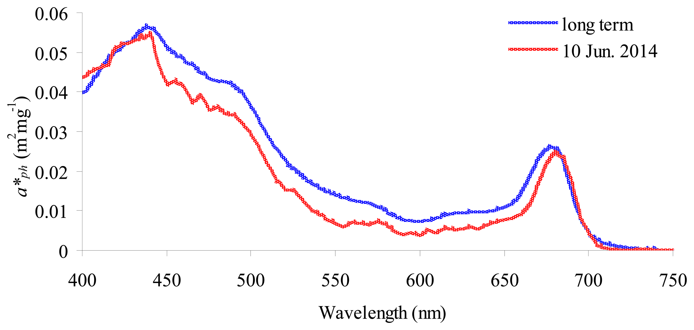
Widely stable water components conditions were encountered with generally low values of concentrations of water constituents. The measured average values in stations 2, 3 and 4 (cf. Figure 1) were 1.01 mg/m3 (±0.32), 0.52 g/m3 (±0.13) and 0.03/m (±0.02), for chl-a, SPM and CDOM, respectively. The total absorption and backscattering coefficients of particles were also indicating the transparency of water. For instance, at 442 nm, ap and bbp were respectively equal to 0.0633 m−1 (±0.0200/m) and to 0.013/m (±0.0003). The SIOPs gathered on 10 June 2014 (Table 2 and Figure 2) were consistent with long term SIOPs mean values [42,43]. In particular, the small differences between the spectra of specific absorption of phytoplankton may reflect the low concentrations of chl-a compared to long term dataset (ranging between 2.3 and 4.0 mg/m3 [47]).
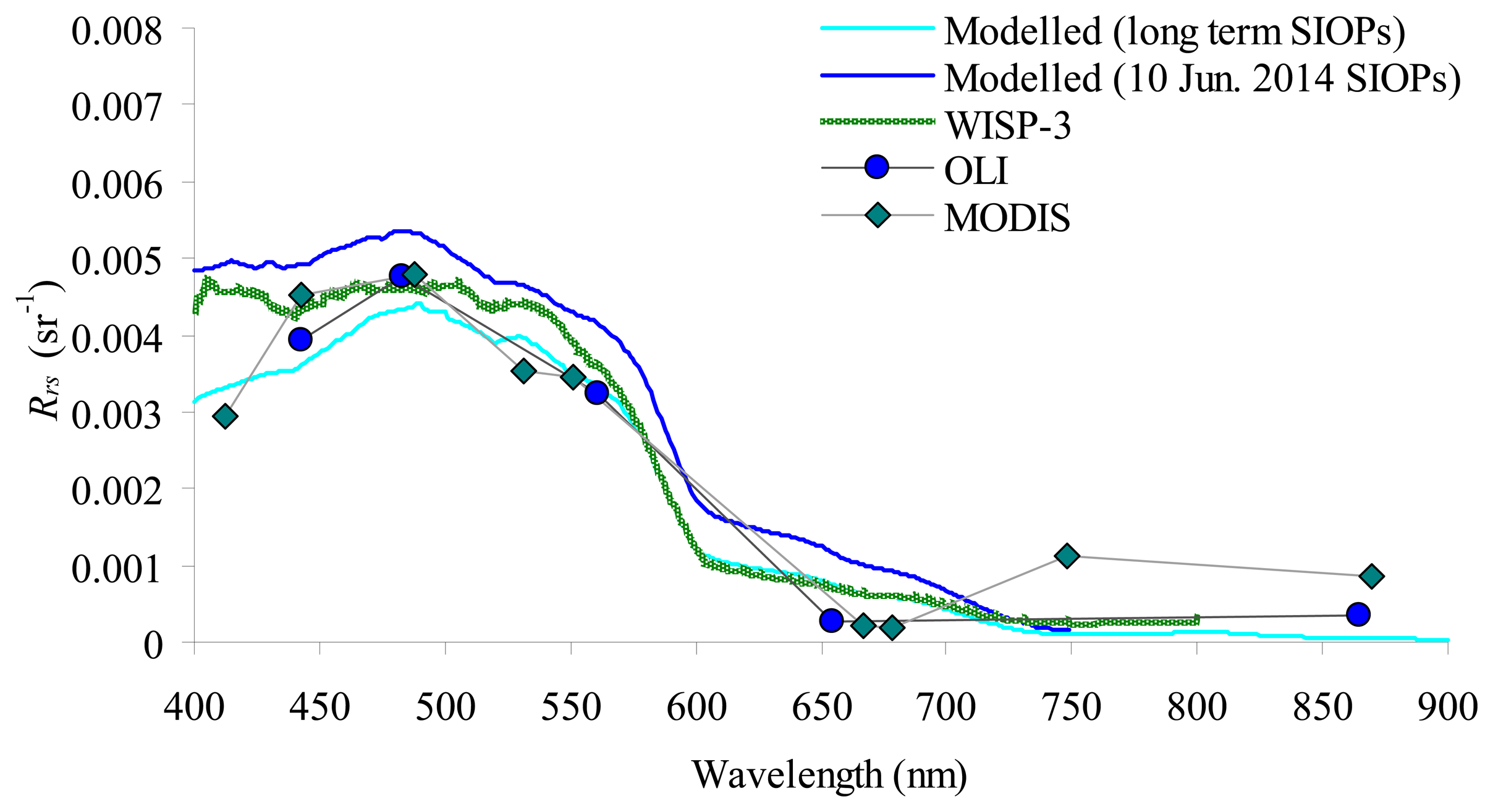
Reliable estimations of water components within such a limited variation range depend on the accuracy and consistency of the parameterization of physics-based processing chain, and it can be assessed with the optical closure between modelled and measured Rrs spectra [5]. Six forward runs of the bio-optical model implemented in BOMBER were performed with all the relevant information gathered from in situ observations. In particular, three runs (one for each station) were performed with concentrations of chl-a, SPM and CDOM and SIOPs gathered on 10 June 2014 (Table 2 and Figure 2); three other runs (one for each station) were performed with the concentrations of chl-a, SPM and CDOM measured on 10 June 2014 and the long term SIOPs (Table 2 [42–44] and Figure 2). The modelled Rrs spectra were compared to the Rrs spectra derived from WISP-3 and atmospherically corrected satellite images respectively. As the change of variation of Rrs spectra between the three stations was very limited, the plot shows the average values only. For MODIS, only the Rrs spectrum corresponding to the most pelagic station (i.e., station 3, cf. Figure 1) was plotted because, for stations 2 and 4, MODIS data were contaminated by the signal coming from the adjacent lands. A feature that, the coarser spatial resolution sensors, already showed in Lake Garda data [40,60].
Figure 3 shows the convergence between modelled and measured Rrs spectra. Overall, the spectra all converge, in particular from 440 to 650 nm where the maximum difference (0.004 sr−1) is between MODIS and WISP-3. For the modelled spectra, a small difference in using the long term SIOPs and the SIOPs gathered on 10 June 2014 was observed, reflecting the small differences between the two SIOP sets (Table 2 and Figure 2). The comparison with WISP-3 showed a better closure by using the Rrs spectra modelled with the SIOPs measured on 10 June 2014, the comparison with 6SV-derived OLI and MODIS spectra instead showed a better closure by using the Rrs spectra modelled with the long term SIOPs. The Rrs divergence was slightly higher for MODIS: in the first channel with a drop and at longer wavelengths with an increase of the signal, probably due to adjacency effects which was anyway present in the most pelagic station.
Based on the optical closure analysis we decided to apply BOMBER: (1) with a parameterisation based on the long term SIOPs (the SIOPs measured on 10 June 2014 were used to validate the satellite-inferred estimation); and (2) in case of MODIS, only for the pixel matching station 3 and by excluding in the inversion process the first and the last two bands (i.e., using the 443–675 nm spectral range).
3.2. Optically Shallow Waters
The optically shallow waters considered in this study were investigated with OLI and RapidEye sensors and in situ data gathered from the two coastal stations (cf. Figure 1): station 1 where SD depth was comparable to the 7-m bathymetry and station 5, where bottom depth was 3 m.
Similarly as for the deeper stations, clear water conditions were encountered. The average concentrations for the two stations for chl-a, SPM and CDOM were 0.74 mg/m3 (±0.13), 0.74 g/m3 (±0.09) and 0.05 m−1 (±0.03), respectively. The absorption coefficient of particle ap at 440 nm and the backscattering coefficient of particles bbp at 442 nm, were respectively equal to 0.0703 m−1 (±0.0190 m−1) and to 0.018 m−1 (±0.0015).
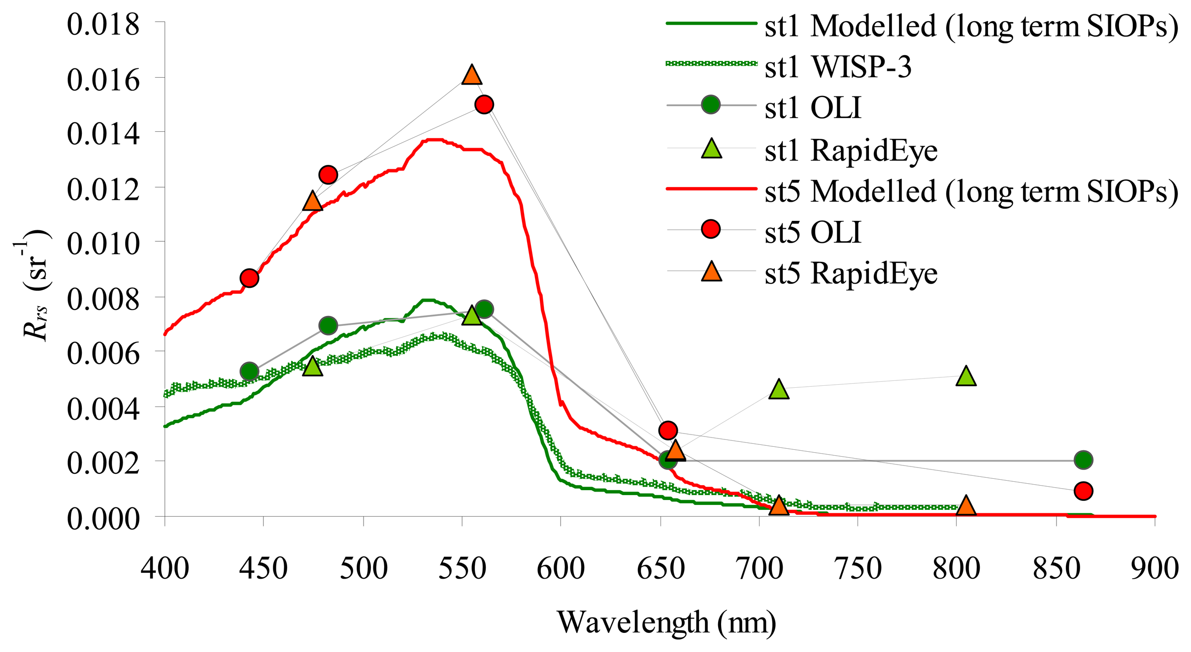
The optical closure in optically shallow waters (Figure 4) was evaluated based on two forward runs of the bio-optical model implemented in BOMBER, with the concentrations of chl-a, SPM and CDOM gathered on 10 June 2014 and the long term SIOPs. The runs were also calibrated with bottom depths measured on 10 June 2014 and bottom albedo based on long term data [42]. The two modelled Rrs spectra were compared to the Rrs spectra derived from WISP-3 (for station 1 only) and satellite images, respectively. In both stations the closure was good, both in terms of magnitude and spectral shapes. Only RapidEye in station 1 was diverging because the station is close to optically deep waters and the sensor noise do not allow smaller signals to be detected [43,61].
Based on the optical closure analysis, the BOMBER was considered suitable for inverting the Rrs spectra measured from OLI and Rapid Eye. Following previous studies [62,63] and due to the homogenous conditions of water constituents measured in situ, BOMBER was run by keeping constant the concentrations of chl-a, SPM and CDOM.
3.3. Validation and Mapping
The results produced by applying BOMBER to satellite images, previously corrected for the atmospheric effects with the 6SV code, were compared to the match-ups with in situ data. Table 3 shows the average values (for the three stations in optically deep waters except for MODIS with results for station 3 only), for the concentrations of chl-a, SPM and CDOM. Comparable results to in situ data were found both from OLI and MODIS, suggesting the capability of the method to assess water quality in clear lake waters.
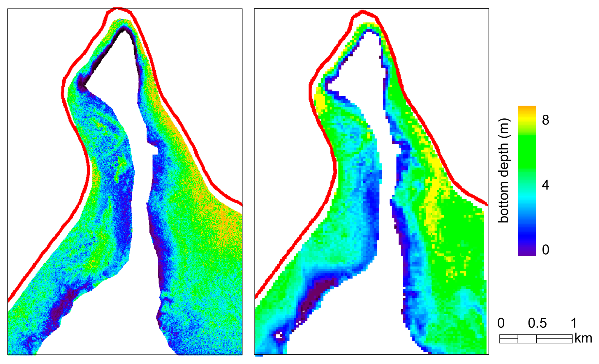
Figure 5 shows the bottom depth maps retrieved from OLI and RapidEye, for waters within the 7-m isobath defined by a nautical chart from 1980. The Pearson correlation coefficient r of the two maps (with RapidEye image resampled according to the spatial resolution of OLI for a total of 5953 samples) was 0.72. The mapped bottom depths from both OLI and RapidEye reached 8 m, which is acceptable by considering that water level of Lake Garda can change of 1.1 m depending on water use and weather conditions [42]. In correspondence of stations 1 and 5, mapped bottom depths from OLI and RapidEye were comparable to in situ observations. In particular, for station 1 (cf. Figure 1), where the SD was 7 m and close to bottom OLI and RapidEye were 6.78 m and 7.10 m, respectively; for station 5, the bottom depth from in situ, RapidEye and OLI was 3 m, 3.2 m and 3.8 m, respectively.
4. Conclusions
A physics-based approach which allows the concentration of water constituents and bottom depth from satellite images to be retrieved has been applied in southern Lake Garda (northern Italy). The method included the correction for the atmospheric effects with the radiative transfer 6SV code [56,57], the evaluation of the environmental noise-equivalent remote sensing reflectance differences NEΔ Rrs(Δ)E according to [58] and the use of the BOMBER tool [55] for estimating the water related products. The images were acquired on 10 June 2014 from MODIS, OLI and RapidEye sensors. During the satellite overpasses fieldwork activities were conducted to gather data for applying the 6SV code, testing the parameterisation of bio-optical model implemented in BOMBER and examining the imagery-derived products.
Very clear water conditions (SD = 8 m) were observed during the image acquisition date with rather low concentrations of water constituents for the season (chl-a = 1.0 mg/m3; SPM = 0.52 g/m3 and CDOM = 0.03 m−1). The NEΔ Rrs(Δ)E analyses suggested that only MODIS and OLI were suitable for assessing such low variation of concentrations. Overall, the results of optical closure showed the good agreement between the 6SV-derived and in situ measured Rrs spectra, with highest divergence in the first MODIS band and in the last two RapidEye channels. The results also showed how MODIS was suitable for investigating the most pelagic station only and consequently not adapted to coastal areas and bathymetric investigations. A set of forward runs of the bio-optical model implemented in BOMBER suggested using the long term SIOPs for estimating both water constituents in the optically deep waters and bottom depths in the shallow waters surrounding the peninsula of Sirmione. The BOMBER-derived products showed good match-ups with in situ data. OLI and MODIS provided chl-a, SPM and CDOM data within the range of in situ measurements; the bottom depth maps from OLI and RapidEye were comparable between them (r = 0.72) and similar to field observations.
This study indicates that the three sensors used have suitable characteristics to support environmental monitoring in Lake Garda. In particular MODIS was appropriate for assessing water quality constituents in the pelagic areas of Lake Garda. By adopting the calibration proposed by Pahlevan et al. [29], OLI was deemed suitable for both optically deep and shallow waters applications as both the spatial and radiometric resolutions enabled a full physics based inversion. Although RapidEye is not specifically designed for aquatic application the study indicated this imagery capability to reproduce lake bottom depth variation.
To confirm the results of this exploratory study, future work should evaluate the performance of the three sensors in different bio-optical conditions. Furthermore, MODIS daily measurements could be used to support of environmental reporting in as demonstrated by Bresciani et al. [14] with MERIS data for European perialpine lakes. To achieve this, a quantitative assessment based on an extended match-up analysis using the long term records should be performed both on the method adopted in this study and on MODIS standard product suites.
Acknowledgments
This study was funded by GLaSS (7th Framework Programme, project number 313256) and CLAM-PHYM (Italian Space Agency, contract nr. I/015/11/0). This study was co-funded by European Union (FP7-People Co-funding of Regional, National and International Programmes, GA n. 600407) and the CNR RITMARE Flagship Project. RapidEye data was made available through the ESA project AO-553 (MELINOS). We are very grateful to Thomas Heege, Mauro Musanti, Gian Luca Fila, Peter Gege and Monica Pinardi for the collaboration and the meaningful conversations on this work, and to two anonymous reviewers for their insightful comments that helped strengthening this manuscript.
Author Contributions
In this work, the general conception has been developed by Claudia Giardino and Mariano Bresciani. Claudia Giardino and Vittorio E. Brando wrote the manuscript and Mariano Bresciani supervised the interpretation of results. Claudia Giardino, Mariano Bresciani, Karin Schenk, Patrizia Rieger, Federica Braga and Vittorio E. Brando participated to fieldwork activities. Image and data processing was performed by Claudia Giardino, Mariano Bresciani and Ilaria Cazzaniga. Erica Matta, and Federica Braga have guaranteed the critical reading.
Conflicts of Interest
The authors declare no conflict of interest.
References
- Lindell, T.; Pierson, D.; Premazzi, G.; Zilioli, E. Manual for Monitoring European Lakes Using Remote Sensing Techniques; EUR Report n. 18665 EN; Joint Research Centre: Ispra, Italy, 1999. [Google Scholar]
- Ritchie, J.C.; Cooper, C.M.; Schiebe, F.R. The relationship of MSS and TM digital data with suspended sediments, chlorophyll, and temperature in Moon Lake, Mississippi. Remote Sens. Environ. 1990, 33, 137–148. [Google Scholar]
- Lathrop, R.G. Landsat thematic mapper monitoring of turbid inland water-quality. Photogram. Engrg. Remote Sens. 1992, 58, 465–470. [Google Scholar]
- Bukata, R.P.; Pozdnyakov, D.V.; Jerome, J.H.; Tanis, F.J. Validation of a radiometric color model applicable to optically complex water bodies. Remote Sens. Environ. 2001, 77, 165–172. [Google Scholar]
- Brando, V.E.; Dekker, A.G. Satellite hyperspectral remote sensing for estimating estuarine and coastal water quality. IEEE Trans. Geosci. Remote Sens. 2003, 41, 1378–1387. [Google Scholar]
- Odermatt, D.; Gitelson, A.; Brando, V.E.; Schaepman, M. Review of constituent retrieval in optically-deep and complex waters from satellite imagery. Remote Sens. Environ. 2012, 118, 116–126. [Google Scholar]
- Chang, N.B.; Daranpob, A.; Yang, Y.J.; Jin, K.R. Comparative data mining analysis for information retrieval of MODIS images: Monitoring lake turbidity changes at Lake Okeechobee, Florida. J. Appl. Remote Sens. 2009, 3. [Google Scholar] [CrossRef]
- Horion, S.; Bergamino, N.; Stenuite, S.; Descy, J.P.; Plisnier, P.D.; Loiselle, S.A.; Cornet, Y. Optimized extraction of daily bio-optical time series derived from MODIS/Aqua imagery for Lake Tanganyika, Africa. Remote Sens. Environ. 2010, 114, 781–791. [Google Scholar]
- Hu, C.; Lee, Z.P.; Ma, R.; Yu, K.; Li, D.; Shang, S. Moderate resolution imaging spectroradiometer (MODIS) observations of cyanobacteria blooms in Taihu Lake, China. J. Geophys. Res. 2010, 115. [Google Scholar] [CrossRef]
- Kaba, E.; Philpot, W.; Steenhuis, T. Evaluating suitability of MODIS-Terra images for reproducing historic sediment concentrations in water bodies: Lake Tana, Ethiopia. Int. J. Appl. Earth Obs. Geoinf. 2014, 26, 286–297. [Google Scholar]
- Zhang, Y.; Lin, S.; Liu, J.; Qian, X.; Ge, Y. Time–series MODIS Image–based retrieval and distribution analysis of total suspended matter concentrations in Lake Taihu (China). Int. J. Environ. Res. Public Health 2010, 7, 3545–3560. [Google Scholar]
- Giardino, C.; Bresciani, M.; Stroppiana, D.; Oggioni, A.; Morabito, G. Optical remote sensing of lakes: An overview on lake Maggiore. J. Limnol. 2014, 73, 201–214. [Google Scholar]
- Odermatt, D.; Pomati, F.; Pitarch, J.; Carpenter, J.; Kawka, M.; Schaepman, M.; Wüest, A. MERIS observations of phytoplankton blooms in a stratified eutrophic lake. Remote Sens. Environ. 2012, 126, 232–239. [Google Scholar]
- Bresciani, M.; Stroppiana, D.; Odermatt, D.; Morabito, G.; Giardino, C. Assessing remotely sensed chlorophyll-a for the implementation of the water framework directive in European perialpine lakes. Sci. Total Environ. 2011, 409, 3083–3091. [Google Scholar]
- Matthews, M.W. Eutrophication and cyanobacterial blooms in South African inland waters: 10 years of MERIS observations. Remote Sens. Environ. 2014, 2014. [Google Scholar] [CrossRef]
- Ali, K.; Witter, D.; Ortiz, J. Application of empirical and semi–analytical algorithms to MERIS data for estimating chlorophyll a in Case 2 waters of Lake Erie. Environ. Earth Sci. 2014, 71, 4209–4220. [Google Scholar]
- Binding, C.E.; Greenberg, T.A.; Bukata, R.P. The MERIS Maximum Chlorophyll Index; its merits and limitations for inland water algal bloom monitoring. J. Great Lakes Res. 2013, 39, 100–107. [Google Scholar]
- Verpoorter, C.; Kutser, T.; Seekell, D.A.; Tranvik, L.J. A global inventory of lakes based on high-resolution satellite imagery. Geophys. Res. Lett. 2014, 41, 6396–6402. [Google Scholar]
- Oyama, Y.; Matsushita, B.; Fukushiman, T. Distinguishing surface cyanobacterial blooms and aquatic macrophytes using Landsat/TM and ETM + shortwave infrared bands. Remote Sens. Environ. 2014, 2014. [Google Scholar] [CrossRef]
- Wu, G.; Cui, L.; Duan, H.; Fei, T.; Liu, Y. An approach for developing Landsat–5 TM–based retrieval models of suspended particulate matter concentration with the assistance of MODIS. ISPRS J. Photogramm. 2013, 85, 84–92. [Google Scholar]
- Dekker, A.G.; Brando, V.E.; Anstee, J.M.; Pinnel, N.; Kutser, T.; Hoogenboom, H.J.; Pasterkamp, R.; Peters, S.W.M.; Vos, R.J.; Olbert, C.; et al. Imaging spectrometry of water. In Imaging Spectrometry: Basic Principles and Prospective Applications; van der Meer, F.D., de Jong, S.M., Eds.; Remote Sensing and Digital Image Processing Dordrecht: Kluwer, The Netherlands, 2001; Volume 4, pp. 307–359. [Google Scholar]
- Giardino, C.; Pepe, M.; Brivio, P.A.; Ghezzi, P.; Zilioli, E. Detecting chlorophyll, Secchi disk depth and surface temperature in a Subalpine lake using Landsat imagery. Sci. Total Environ. 2001, 268, 19–29. [Google Scholar]
- Brivio, P.A.; Giardino, C.; Zilioli, E. Determination of chlorophyll concentration changes in Lake Garda using an image-based radiative transfer code for Landsat TM images. Int. J. Remote Sens. 2001, 22, 487–502. [Google Scholar]
- Torbick, N.; Hession, S.; Hagen, S.; Wiangwang, N.; Becker, B.; Qi, J. Mapping inland lake water quality across the Lower Peninsula of Michigan using Landsat TM imagery. Int. J. Remote Sens. 2013, 34, 7607–7624. [Google Scholar]
- Brezonik, P.L.; Menken, K.; Bauer, M.E. Landsat-based remote sensing of lake water quality characteristics, including chlorophyll and colored dissolved organic matter (CDOM). Lake Reserv. Manage. 2005, 21, 373–382. [Google Scholar]
- Tebbs, E.J.; Remedios, J.J.; Harper, D.M. Remote sensing of chlorophyll-a as a measure of cyanobacterial biomass in Lake Bogoria, a hypertrophic, saline–alkaline, flamingo lake, using Landsat ETM+. Remote Sens. Environ. 2013, 135, 92–106. [Google Scholar]
- Dekker, A.G.; Brando, V.E.; Anstee, J.M. Retrospective seagrass change detection in a shallow coastal tidal Australian lake. Remote Sens. Environ. 2005, 97, 415–433. [Google Scholar]
- Lobo, F.L.; Costa, M.P.F.; Novo, E.M.L.M. Time-series analysis of Landsat-MSS/TM/OLI images over Amazonian waters impacted by gold mining activities. Remote Sens. Environ. 2014, 2014. [Google Scholar] [CrossRef]
- Pahlevan, N.; Lee, Z.; Wei, J.; Schaaf, C.B.; Schott, J.R.; Berk, A. On-orbit radiometric characterization of OLI (Landsat-8) for applications in aquatic remote sensing. Remote Sens. Environ. 2014, 154, 272–284. [Google Scholar]
- Moufid, T. SNR Characterization in RapidEye Satellite Images. Master's Thesis, Space Engineering-Space Master, Luleå University of Technology, Luleå, Sweden, 22 September 2014. [Google Scholar]
- Chang, C.W.; Salinas, S.V.; Liew, S.C.; Lee, Z. Atmospheric correction of IKONOS with cloud and shadow image features. Proceedings of the Geoscience and Remote Sensing Symposium, Barcelona, Spain, 23–28 July 2007; pp. 875–878.
- Lee, Z.; Weidemann, A.; Arnone, R. Combined Effect of reduced band number and increased bandwidth on shallow water remote sensing: The case of worldview 2. IEEE Trans. Geosci. Remote Sens. 2013, 51, 2577–2586. [Google Scholar]
- Su, H.; Liu, H.; Wang, L.; Filippi, A.M.; Heyman, W.D.; Beck, R.A. Geographically Adaptive inversion model for improving bathymetric retrieval from satellite multispectral imagery. IEEE Trans. Geosci. Remote Sens. 2014, 52, 465–476. [Google Scholar]
- Paringit, E.C.; Nadaoka, K. Simultaneous estimation of benthic fractional cover and shallow water bathymetry in coral reef areas from high-resolution satellite images. Int. J. Remote Sens. 2012, 33, 3026–3047. [Google Scholar]
- Lyons, M.; Phinn, S.; Roelfsema, C. Integrating Quickbird multi-spectral satellite and field data: Mapping bathymetry, seagrass cover, seagrass species and change in Moreton Bay, Australia in 2004 and 2007. Remote Sens. 2011, 3, 42–64. [Google Scholar]
- Su, H.; Liu, H.; Heyman, W.D. Automated derivation of bathymetric information from multi-spectral satellite imagery using a non-linear inversion model. Mar. Geod. 2008, 31, 281–298. [Google Scholar]
- Vahtmäe, E.; Kutser, T. Mapping bottom type and water depth in shallow coastal waters with satellite remote sensing. J. Coast. Res. 2007, 50, 185–189. [Google Scholar]
- Bresciani, M.; Giardino, C.; Boschetti, L. Multi-temporal assessment of bio-physical parameters in lakes Garda and Trasimeno from MODIS and MERIS. Ital. J. Remote Sens. 2011, 43, 49–62. [Google Scholar]
- Guanter, L.; Ruiz-Verdù, A.; Odermatt, D.; Giardino, C.; Simis, S.; Estellès, V.; Heege, T.; Domìnguez-Gòmez, J.A.; Moreno, J. Atmospheric correction of ENVISAT/MERIS data over inland waters: Validation for European lakes. Remote Sens. Environ. 2010, 114, 467–480. [Google Scholar]
- Odermatt, D.; Giardino, C.; Heege, T. Chlorophyll retrieval with MERIS Case-2-Regional in Perialpine Lakes. Remote Sens. Environ. 2010, 114, 607–617. [Google Scholar]
- Giardino, C.; Bresciani, M.; Valentini, E.; Gasperini, L.; Bolpagni, R.; Brando, V.E. Airborne hyperspectral data to assess suspended particulate matter and aquatic vegetation in a shallow and turbid lake. Remote Sens. Environ. 2014, 2014. [Google Scholar] [CrossRef]
- Bresciani, M.; Bolpagni, R.; Braga, F.; Oggioni, A.; Giardino, C. Retrospective assessment of macrophytic communities in southern Lake Garda (Italy) from in situ and MIVIS (Multispectral Infrared and Visible Imaging Spectrometer) data. J. Limnol. 2012, 71, 180–190. [Google Scholar]
- Giardino, C.; Bartoli, M.; Candiani, G.; Bresciani, M.; Pellegrini, L. Recent changes in macrophyte colonisation patterns: An imaging spectrometry-based evaluation of southern Lake Garda (northern Italy). J. Appl. Remote Sens. 2007, 1. [Google Scholar] [CrossRef]
- Giardino, C.; Brando, V.E.; Dekker, A.G.; Strömbeck, N.; Candiani, G. Assessment of water quality in Lake Garda (Italy) using Hyperion. Remote Sens. Environ. 2007, 109, 183–195. [Google Scholar]
- Salmaso, N.; Mosello, R. Limnological research in the deep southern subalpine lakes: Synthesis, directions and perspectives. Adv. Oceanogr. Limnol. 2010, 1, 29–66. [Google Scholar]
- Vollenweider, R.A.; Kerekes, J.J. Eutrophication of Waters: Monitoring Assessment and Control; Organisation for Economic Co–operation and Development: Paris, France, 1982; p. 150. [Google Scholar]
- Salmaso, N. Long-term phytoplankton community changes in a deep subalpine lake: Responses to nutrient availability and climatic fluctuations. Freshwater Biol. 2010, 55, 825–846. [Google Scholar]
- Lorenzen, C.J. Determination of chlorophyll and pheo-pigments: Spectrophotometric equations. Limnol. Oceanogr. 1967, 12, 343–346. [Google Scholar]
- Strömbeck, N.; Pierson, E. The effects of variability in the inherent optical properties on estimations of chlorophyll a by remote sensing in Swedish freshwaters. Sci. Total Environ. 2001, 268, 123–137. [Google Scholar]
- Kirk, J.T.O. Light & Photosynthesis in Aquatic Ecosystems, 2nd ed.; Cambridge University Press: New York, NY, USA, 1994; p. 509. [Google Scholar]
- Maffione, R.A.; Dana, D.R. Instruments and methods for measuring the backward-scattering coefficient of ocean waters. Appl. Optics 1997, 36, 6057–6067. [Google Scholar]
- Cracknell, A.P.; Newcombe, S.K.; Black, A.F. The ABDMAP (algal bloom detection, monitoring and prediction). Int. J. Remote Sens. 2001, 22, 205–247. [Google Scholar]
- Mobley, C.D. Light and Water: Radiative Transfer in Natural Waters; Academic Press: San Diego, CA, USA, 1994. [Google Scholar]
- Berk, A.; Bernsten, L.S.; Robertson, D.C. MODTRAN: A Moderate Resolution Model for LOWTRAN7; Report GL–TR–89–0122; Air Force Geophysics Laboratory: Bedford, MA, USA, 1989; p. 38. [Google Scholar]
- Giardino, C.; Candiani, G.; Bresciani, M.; Lee, Z.; Gagliano, S.; Pepe, M. BOMBER: A tool for estimating water quality and bottom properties from remote sensing images. Comput. Geosci. 2012, 45, 313–318. [Google Scholar]
- Kotchenova, S.Y.; Vermote, E.F.; Matarrese, R.; Klemm, F.J., Jr. Validation of a vector version of the 6S radiative transfer code for atmospheric correction of satellite data. Part I: Path radiance. Appl. Opt. 2006, 45, 6762–6774. [Google Scholar]
- Kotchenova, S.Y.; Vermote, E.F. Validation of a vector version of the 6S radiative transfer code for atmospheric correction of satellite data. Part II. Homogeneous Lambertian and anisotropic surfaces. Appl. Opt. 2007, 46, 4455–4464. [Google Scholar]
- Wettle, M.; Brando, V.E.; Dekker, A.G. A methodology for retrieval of environmental noise equivalent spectra applied to four Hyperion scenes of the same tropical coral reef. Remote Sens. Environ. 2004, 93, 188–197. [Google Scholar]
- Hu, C.; Feng, L.; Lee, Z.; Davis, C.; Mannino, A.; McClain, C.; Franz, B. Dynamic range and sensitivity requirements of satellite ocean color sensors: Learning from the past. Appl. Opt. 2012, 51, 6045–6062. [Google Scholar]
- Candiani, G.; Giardino, C.; Brando, V.E. Adjacency effects and bio–optical model regionalisation: meris data to assess lake water quality in the subalpine ecoregion. Proceeding of the Envisat Symposium, Montreux, Switzerland, 23–27 April 2007.
- Brando, V.E.; Anstee, J.M.; Wettle, M.; Dekker, A.G.; Phinn, S.R.; Roelfsema, C. A physics based retrieval and quality assessment of bathymetry from suboptimal hyperspectral data. Remote Sens. Environ. 2009, 113, 755–770. [Google Scholar]
- Adler-Golden, S.M.; Acharya, P.K.; Berk, A.; Matthew, M.W.; Gorodetzky, D. Remote bathymetry of the littoral zone from AVIRIS, LASH, and QuickBird imagery. IEEE Trans. Geosci. Remote Sens. 2005, 43, 337–347. [Google Scholar]
- Dierssen, H.M.; Zimmerman, R.C. Ocean color remote sensing of seagrass and bathymetry in the Bahamas Banks by high-resolution airborne imagery. Limnol. Oceanogr. 2003, 48, 444–455. [Google Scholar]


| Satellite | Data Access | UTC | Pixel Size (m) | Number of Bands | NEΔRrs(Δ)E |
|---|---|---|---|---|---|
| Aqua MODIS | Ocean Colour 1 | 12:50 | 1000 | 9 | 0.018% |
| Landsat 8 OLI | GLOVIS 2 | 10:04 | 30 | 5 | 0.010% |
| RapidEye 3 (Choma) | EOLI-SA 3 | 11:13 | 5 | 5 | 0.221% |
1 oceancolor.gsfc.nasa.gov;2 glovis.usgs.gov/;3 earth.esa.int/EOLi/EOLi.html.
| Coefficient | 10 June 2014 | Long Term |
|---|---|---|
| Spectral slope coefficient of the exponential CDOM absorption (nm−1) curve | 0.025 | 0.021 |
| Specific absorption of NAP at 440 nm (m2/g) | 0.031 | 0.050 |
| Spectral slope coefficient of the exponential NAP absorption (nm−1) curve | 0.012 | 0.012 |
| Specific backscattering coefficient of SPM at 555 nm (m2/g) | 0.0082 | 0.0071 |
| Backscattering exponent of the power-law SPM curve | 0.64 | 0.76 |
| Data Source | chl-a (mg/m3) | SPM (g/m3) | CDOM (m−1) |
|---|---|---|---|
| In situ | 1.01 (±0.32) | 0.52 (±0.13) | 0.03 (±0.02) |
| OLI | 1.04 (±0.10) | 0.69 (±0.08) | 0.02 (±0.004) |
| MODIS | 0.83 | 0.41 | 0.01 |
© 2014 by the authors; licensee MDPI, Basel, Switzerland. This article is an open access article distributed under the terms and conditions of the Creative Commons Attribution license ( http://creativecommons.org/licenses/by/4.0/).
Share and Cite
Giardino, C.; Bresciani, M.; Cazzaniga, I.; Schenk, K.; Rieger, P.; Braga, F.; Matta, E.; Brando, V.E. Evaluation of Multi-Resolution Satellite Sensors for Assessing Water Quality and Bottom Depth of Lake Garda. Sensors 2014, 14, 24116-24131. https://doi.org/10.3390/s141224116
Giardino C, Bresciani M, Cazzaniga I, Schenk K, Rieger P, Braga F, Matta E, Brando VE. Evaluation of Multi-Resolution Satellite Sensors for Assessing Water Quality and Bottom Depth of Lake Garda. Sensors. 2014; 14(12):24116-24131. https://doi.org/10.3390/s141224116
Chicago/Turabian StyleGiardino, Claudia, Mariano Bresciani, Ilaria Cazzaniga, Karin Schenk, Patrizia Rieger, Federica Braga, Erica Matta, and Vittorio E. Brando. 2014. "Evaluation of Multi-Resolution Satellite Sensors for Assessing Water Quality and Bottom Depth of Lake Garda" Sensors 14, no. 12: 24116-24131. https://doi.org/10.3390/s141224116