The Effects of Aerosol on the Retrieval Accuracy of NO₂ Slant Column Density

Abstract

We investigate the effects of aerosol optical depth (AOD), single scattering albedo (SSA), aerosol peak height (APH), measurement geometry (solar zenith angle (SZA) and viewing zenith angle (VZA)), relative azimuth angle, and surface reflectance on the accuracy of NO₂ slant column density using synthetic radiance. High AOD and APH are found to decrease NO₂ SCD retrieval accuracy. In moderately polluted (5 × 10¹⁵ molecules cm⁻² < NO₂ vertical column density (VCD) < 2 × 10¹⁶ molecules cm⁻²) and clean regions (NO₂ VCD < 5 × 10¹⁵ molecules cm⁻²), the correlation coefficient (R) between true NO₂ SCDs and those retrieved is 0.88 and 0.79, respectively, and AOD and APH are about 0.1 and is 0 km, respectively. However, when AOD and APH are about 1.0 and 4 km, respectively, the R decreases to 0.84 and 0.53 in moderately polluted and clean regions, respectively. On the other hand, in heavily polluted regions (NO₂ VCD > 2 × 10¹⁶ molecules cm⁻²), even high AOD and APH values are found to have a negligible effect on NO₂ SCD precision. In high AOD and APH conditions in clean NO₂ regions, the R between true NO₂ SCDs and those retrieved increases from 0.53 to 0.58 via co-adding four pixels spatially, showing the improvement in accuracy of NO₂ SCD retrieval. In addition, the high SZA and VZA are also found to decrease the accuracy of the NO₂ SCD retrieval.

1. Introduction

Nitrogen dioxide (NO₂) is an important atmospheric trace gas because it adversely affects human health and plays a key role in the photochemistry of ozone [1,2]. Differential Optical Absorption Spectroscopy (DOAS) [3], which is a method to retrieve total amounts of atmospheric trace gases through the remote sensing measurement of light in the ultra violet, visible, and near infrared spectral range, is widely used to monitor NO₂ using both ground-based remote sensing measurements, such as Multi-Axis DOAS, and space-born instruments such as the Global Ozone Monitoring Experiment (GOME) [4], the Scanning Imaging Spectrometer for Atmospheric Cartography (SCIAMACHY), the Ozone Monitoring Instrument (OMI) [5,6], and GOME-2 [2,7]. The key idea of the DOAS method is to separate broad and narrow band spectral structures of the absorption spectra in order to find the narrow trace gas absorption features.

In polluted regions, the estimated uncertainties of the OMI DOAS NO₂ algorithm are about 30% and 60% in clear and partly cloudy conditions, respectively [8]. The estimated uncertainty in the GOME-2 tropospheric NO₂ algorithm ranges from 40% to 80% [7]. The causes of these NO₂ retrieval errors are mainly air mass factor (AMF) and spectral fitting errors.

The NO₂ AMF error is mainly caused by uncertainties in the NO₂ profile shape, surface albedo, cloud information, and aerosol information [7,9,10,11]. Boersma et al. [9] reported that the accuracy of tropospheric AMF depends on the a priori NO₂ profile shape and four model parameters: cloud fraction, cloud (top) height, surface albedo, and the aerosol optical thickness profile. Leitão et al. [10] and Hong et al. [11] reported large effects of the aerosol layer height on NO₂ AMF. According to Valks et al. [7], uncertainties in the tropospheric NO₂ AMF in polluted regions due to uncertainties in cloud fraction, cloud top pressure, and a priori NO₂ profile are 25%, 30% and 10%, respectively.

These spectral fitting errors occur due to uncertainties in the NO₂ cross-section, spectral calibration, and instrument noise, such as dark current and stray light. Boersma et al. [9] reported that various laboratory measurements of NO₂ cross-section, spectral calibration, and estimated chemical transfer model (CTM) temperature precision lead to slant column errors of 2%, 0.5%, and 2%, respectively. Boersma et al. [12] and Valks et al. [7] reported that the OMI (spatial resolution = 13 × 24 km) NO₂ slant column density (SCD) error is 6.7 × 10¹⁴ molecules cm⁻², while that of GOME2 (spatial resolution = 40 × 40 km) SCD is 3.5 × 10¹⁴ molecules cm⁻². Irie et al. [13] quantified the effects of sensor attributes such as signal-to-noise ratio (SNR), full width at half maximum (FWHM), and sampling ratio on NO₂ SCD precision.

Many previous studies have investigated uncertainties in DOAS NO₂ retrieval in terms of atmospheric and surface condition, thus AMF and spectroscopy of the fitting method (fitting uncertainty). However, their cross effects on the other factors (i.e., aerosol effects on NO₂ SCD fitting precision) still remain uncertain. This study investigates the effects of aerosol properties (aerosol optical depth (AOD), single scattering albedo (SSA), aerosol peak height (APH)), measurement geometry (solar zenith angle (SZA), and relative azimuth angle (RAA)), and surface reflectance (SFR) on the NO₂ SCD precision for DOAS NO₂ retrieval at various SNR and NO₂ levels. Changes in NO₂ SCD precision are also investigated using a spatial co-adding technique.

2. Methodology

Figure 1 shows a flowchart of the NO₂ SCD precision test using the DOAS method. This flowchart includes the computation of the AMF and a synthetic radiance. The NO₂ SCD is retrieved from the synthetic radiance. The AMF calculation is carried out using the linearized pseudo-spherical scalar and vector discrete ordinate radiative transfer (VLIDORT, version 2.6) method [14]. The vertical profiles of NO₂, temperature, and pressure data are obtained from the Model of Ozone and Related Chemical Tracers version 4 (MOZART-4). Other gas vertical profiles, such as ozone, are obtained from Deriving Information of Surface Conditions from Column and Vertically Resolved Observations Relevant to Air Quality (Discover-AQ) data.

To understand which parameters affect NO₂ SCD precision, four steps were taken. First, a total of 729 synthetic radiances were generated using VLIDORT from 422 to 460 nm with 0.2 nm sampling resolution, and the AMF was computed under fixed NO₂ vertical column density (VCD) with various values of AOD, SSA, SFR, SZA, RAA, and APH (

Table 1. Variables used to calculate synthetic radiances and AMF, and their values. (air mass factor (AMF), vertical column density (VCD), aerosol optical depth (AOD), single scattering albedo (SSA), aerosol peak height (APH), solar zenith angle (SZA), viewing zenith angle (VZA), relative azimuth angle (RAA), and surface reflectance (SFR)).

Variables	Value
NO2 VCD	5 × 1016 molec. cm−2
	1 × 1016 molec. cm−2
	7.5 × 1015 molec. cm−2
	5 × 1015 molec. cm−2
	2.5 × 1015 molec. cm−2
	1 × 1015 molec. cm−2
	9 × 1014 molec. cm−2
	8 × 1014 molec. cm−2
	7 × 1014 molec. cm−2
	6 × 1014 molec. cm−2
	5 × 1014 molec. cm−2
AOD	0.1, 0.5, 1
SSA	0.999, 0.900, 0.820
APH	0 km, 2 km, 4 km
AMFG (SZA or VZA) = sec(SZA) + sec(VZA)	2.3 (20°, 40°), 2.6 (40°, 40°), 4.2 (40°, 70°)
RAA	0°, 90°, 180°
SFR	0.04, 0.08, 0.12

).

The aerosol profile is based on a Gaussian distribution function (GDF), as used by [11,15] and the equation of the GDF is as follow:

$$\mathrm{GDF}={{\displaystyle \int }}_{{\mathrm{z}}_{\mathrm{n}1}}^{{\mathrm{z}}_{\mathrm{n}2}}\mathrm{W}\frac{{\mathrm{e}}^{-\mathrm{h}\left(\mathrm{z}-{\mathrm{z}}_{\mathrm{p}}\right)}}{{\left[1+{\mathrm{e}}^{-\mathrm{h}\left(\mathrm{z}-{\mathrm{z}}_{\mathrm{p}}\right)}\right]}^2}$$

(1)

$$\mathsf{\eta }=\frac{\ln \left(3+\sqrt{8}\right)}{\mathrm{h}}$$

(2)

where W is a normalization constant related to total aerosol loading, and z_n1 and z_n2 are the aerosol lower and upper limits, respectively. Z_p is the APH and h is related to the half width η [14]. The model input values such as fine and coarse-mode radii, and number fine-mode fraction can be found in [11,15]. A total of 729 (3⁶) synthetic radiances were calculated from six variables with three values for each variable, as listed in Table 1. The AMF was calculated at 440 nm, which is the center of the fitting window. The NO₂ profiles used are shown in Figure 2, and the ranges of NO₂ VCD and model input parameters, such as AOD and SSA, are summarized in Table 1. The NO₂ profiles was calculated from NO₂ shape factor in Beijing during December 2011 obtained from MOZART-4.

Secondly, random noise (SNR from 1000 to 3000 in steps of 500) was added to the calculated synthetic radiances. These synthetic radiances were convoluted with the Gaussian slit function with various full-width-half-maximums (0.2, 0.4, 0.6, and 0.8). The SNR of each synthetic radiance was calculated using the following equation [16]:

$${\mathrm{SNR}}_i\left(\mathsf{\lambda }\right)={\mathrm{SNR}}_a\times \sqrt{\frac{I_i\left(\lambda \right)}{I_a}}$$

(3)

where ${\mathrm{SNR}}_i\left(\mathsf{\lambda }\right)$ and $I_i\left(\lambda \right)$ are the ith SNR and radiance at wavelength λ, respectively. $I_a$ is the average value of all synthetic radiances (about 1.7 × 10¹³ photons (s⁻¹ cm⁻² nm⁻¹)) from 422 to 460 nm, and ${\mathrm{SNR}}_a$ is its corresponding SNR.

Figure 3a shows synthetic radiances calculated using VLIDORT under the following conditions: NO₂ column of 5 × 10¹⁵ molecules cm⁻², SZA (VZA) of 20° (20°), RAA of 50°, surface reflectance of 0.04, APH of 0 km, and SSA of 0.95. Random noise (SNR = 2000) was added to each synthetic radiance. The black circles, blue squares, and red triangles represent the synthetic radiance intensity at AOD of 0.1, 0.5, and 1, respectively. Radiance intensity increases with increasing AOD. Figure 3b is the same as Figure 3a, but with AOD of 1.0 and varying APH conditions. The black circles, blue squares, and red triangles represent synthetic radiance intensity at APH of 0, 2, and 4 km, respectively.

Thirdly, a total of 729 NO₂ SCD were retrieved from 729 synthetic radiances for the individual NO₂ VCD values listed in Table 1 using QDOAS software developed at the Royal Belgian institute for Space Aeronomy (BIRA-IASB) [17]. Spectral fitting was performed between 432 and 450 nm. The NO₂ cross-section from BIRA-IASB no2r_97 [18] and ozone cross-section from SCIAMACHY vacuum calculations [19] were used in the fitting procedure. The example of optical density and residual are shown in Figure 4.

Finally, the retrieved NO₂ SCDs were compared with the true NO₂ SCDs (Figure 1). The NO₂ SCD error, which is the difference between the retrieved and true NO₂ SCDs, occurs only due to the spectral fitting, since we used true AMF values in this study.

3. Results

3.1. No-Noise Conditions

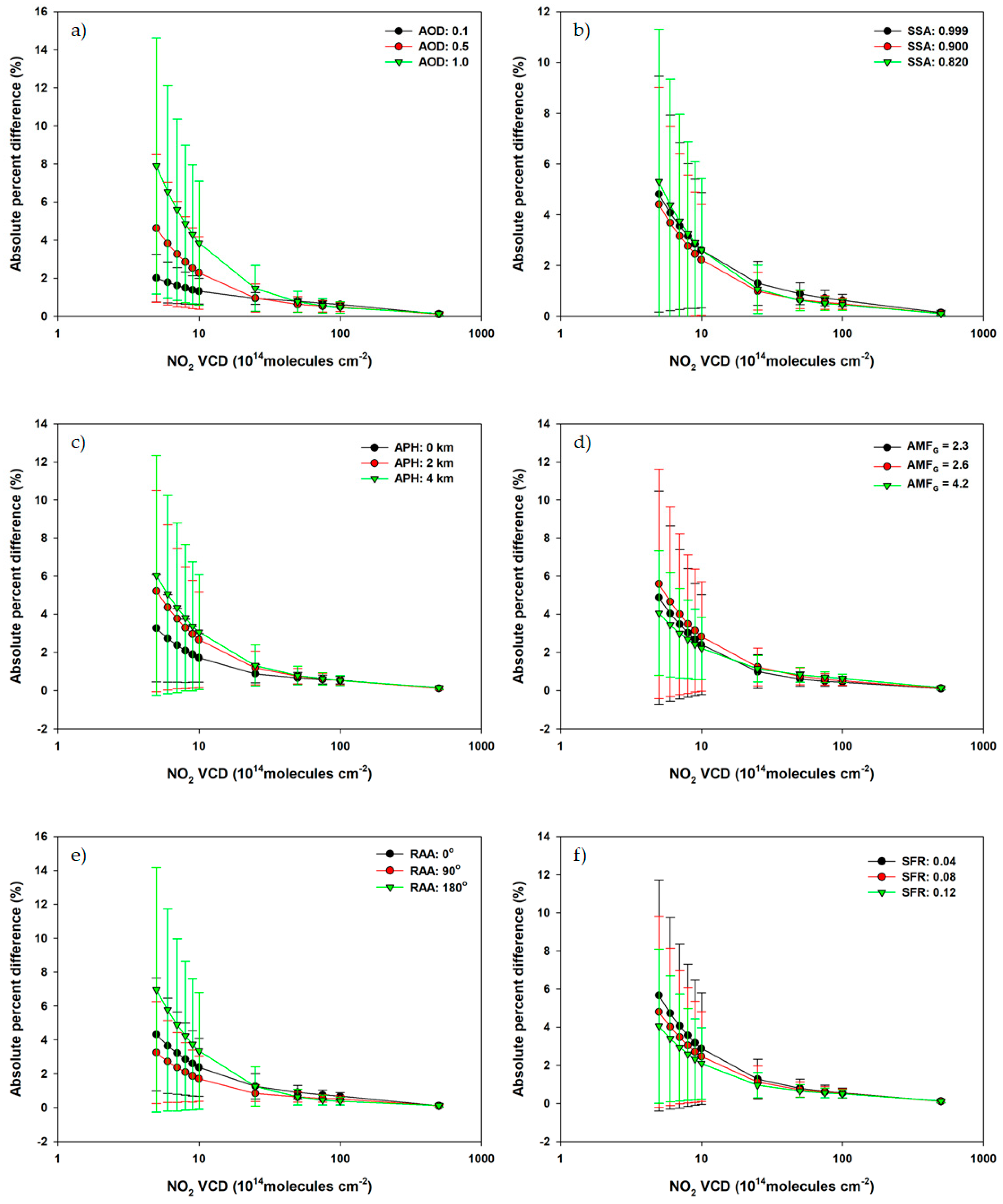
To investigate the effects of AOD, SSA, APH, SZA, RAA, and SFR on NO₂ SCD precision, NO₂ SCDs were retrieved using the DOAS method from various synthetic radiances under no-noise conditions and FWHM of 0.6 nm. Figure 5a shows the absolute percentage difference (APD) between the retrieved and true NO₂ SCDs, as calculated by multiplying the input NO₂ VCD (Table 1) by the AMF, which was computed using VLIDORT (Figure 1). Each black circle, red circle, and green inverted triangle indicate the average of the 243 APD obtained using an AOD of 0.1, 0.5, and 1.0, and every value for the remaining five variables listed in Table 1, respectively. Figure 5b–f is the same as Figure 5a but for varying SSA, APH, AMF_G, RAA, and SFR. The APDs in all cases are less than 2% when NO₂ VCD is greater than 2.5 × 10¹⁵ molecules cm⁻². However, the APD increases to 7.89% when NO₂ VCD is less than 1 × 10¹⁵ molecules cm⁻².

Increasing AOD and APH leads to an increase in APD. The average APD and standard deviation of APD with AOD of 0.1 under all NO₂ VCD conditions listed in Table 1 are about 1.15% and 0.57%, respectively. However, with an AOD of 1.0, these values increase to 3.31% (average) and 2.79% (standard deviation). Similarly, when APH is 0 km, the APD is about 1.52% (average) and 1.16% (standard deviation), but when APH reaches 4 km, these values increase to 2.64% (average) and 2.59% (standard deviation). The average APD and standard deviation of APD with a RAA of 0° are about 2.07% and 1.46%, respectively, whereas with an RAA of 180° these values increase to 2.89% and 2.93%, respectively. A similar increase in both average and standard deviation of APD is found with increasing AMF_G and RAA, which could be associated with the absorption light path change due to the change of aerosol scattering angle. It is subject to further study to quantify the effect of scattering phase function on the NO₂ SCD precision in terms of various aerosol conditions.

However, increasing SFR is found to decrease the APD. Degraded NO₂ SCD retrieval precision occurs under conditions of large AOD, APH, and RAA. It is thought that this degradation is caused by an increase in NO₂ fitting errors resulting from the use of polynomials to explain the Mie (or Rayleigh) scattering efficiency that do not fully reflect aerosol effects at large AOD, APH, and RAA.

3.2. Noise Conditions

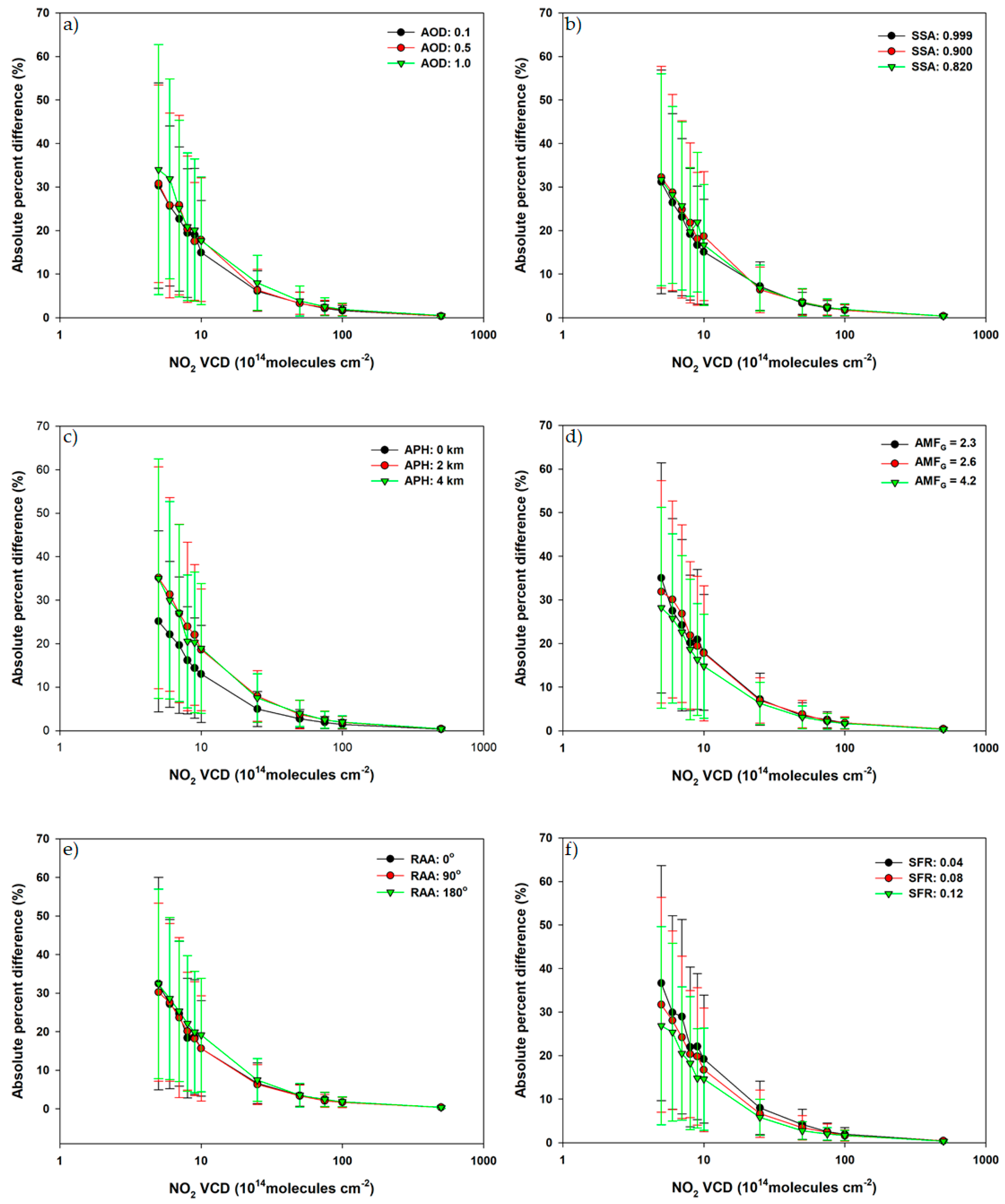
We added random noise (SNR = 2000) to the synthetic radiance to investigate the effects of model input parameters under real conditions. Figure 6 shows the resulting APD between the retrieved and true NO₂ SCDs as a function of NO₂ VCD under noisy conditions. The APDs in all cases are lower than 1.97% under high-NO₂ conditions (NO₂ VCD > 1 × 10¹⁶ molecules cm⁻²), whereas APD undergoes large increases (up to 36.65% in the case of SFR = 0.04) with decreasing NO₂.

When the AOD is 0.1 (1.0), average APD is 6.12% (7.96%), 14.94% (17.66%), 19.04% (20.10%), 19.44% (20.88%), 22.67% (25.08%), 25.65% (31.89%), and 30.32% (34.01%) under conditions of NO₂ VCD of 25, 10, 9, 8, 7, 6, and 5 × 10¹⁴ molecules cm⁻², respectively (Figure 6a). Large errors in NO₂ retrieval using the DOAS method may be present in the background region due to low SCD retrieval precision. Irie et al. [13] reported the retrieval detection limit of NO₂ column density using the DOAS method to about 6 × 10¹⁴ molecules cm⁻² when the SNR at 450 nm is 2000, the FWHM is 0.6 nm, and the AOD is 0.1. However, as shown in Figure 6, not only SNR and FWHM but also aerosol properties, especially APH, affect NO₂ SCD precision.

Figure 7 shows the APD between true and retrieved NO₂ SCDs as a function of NO₂ VCD under various SNR conditions (no error and SNR of 1000, 1500, 2000, 2500, and 3000) at FWHM of 0.6 nm. The APD shows a significant increase with decreasing SNR.

Under no-error conditions, the APD only increases from 0.12% to 4.84% as NO₂ VCD decreases from 5 × 10¹⁶ to 5 × 10¹⁴ molecules cm⁻², whereas with a SNR of 1000 (2000; 3000), the APD increases from 0.72% (0.38%; 0.26%) to 65.42% (33.43%; 23.10%) as NO₂ VCD decreases from 5 × 10¹⁶ to 5 × 10¹⁴ molecules cm⁻². When NO₂ VCD is 5 × 10¹⁵ molecules cm⁻², the APDs with a SNR of 1000, 2000, and 3000 are 6.79%, 3.46%, and 2.47%, respectively.

3.3. Investigation of the Effects of AOD and APH on NO₂ SCD Precision Under Real Conditions

To examine the effects of AOD and APH on NO₂ SCD precision, NO₂ SCD was retrieved using the DOAS method in heavily polluted, moderately polluted, and clean regions. Heavily polluted, moderately polluted, and clean regions are defined as having a NO₂ VCD of over 2 × 10¹⁶ molecules cm⁻², between 5 × 10¹⁵ and 2 × 10¹⁶ molecules cm⁻², and under 5 × 10¹⁵ molecules cm⁻², respectively (

Table 2. NO₂ column range and case study areas in heavily polluted, moderately polluted, and clean regions, along with AOD and APH ranges used to calculate AMF and synthetic radiances under low- and high-AOD conditions. (Aerosol optical depth (AOD), aerosol peak height (APH) and air mass factor (AMF)).

Category	NO2 Column Range	Case Study Area	Low-AOD Condition	High-AOD Condition
Heavily polluted regions	>2 × 1016 molecules cm−2	Hong Kong-Macau	0.16 < AOD < 0.24	0.8 < AOD < 1.2
			APH = 0 km	APH = 4 km
		Tokyo, Osaka	0.09 < AOD < 0.12	0.9 < AOD < 1.2
			APH = 0 km	APH = 4 km
Moderately polluted regions	>5 × 1015 molecules cm−2	Japan (except Tokyo and Osaka)	0.09 < AOD < 0.12	0.9 < AOD < 1.2
	<2 × 1016 molecules cm−2		APH = 0 km	APH = 4 km
Clean regions	<5 × 1015 molecules cm−2	Manila	AOD = 0.02	AOD = 1.0
			APH = 0 km	APH = 4 km

). The Hong Kong-Macau region, Tokyo, and Osaka were selected as heavily polluted regions. The remaining regions of Japan were selected as moderately polluted, including the Honshu region, where high AOD and APH are frequently observed in spring, as Japan is downwind of Asian yellow dust sources [20,21], and the spatial distributions of NO₂ over these regions vary considerably [22]. Manila was selected to represent clean regions.

The NO₂ precision test was carried out in December 2011 because of high observed NO₂ VCD in the Northern Hemisphere during winter [23]. The effects of AOD and APH on NO₂ SCD under both low- and high-AOD conditions were also investigated. Under low-AOD conditions, AMF and synthetic radiance were calculated using monthly averaged Moderate Resolution Imaging Spectroradiometer (MODIS) AOD data for December 2011 and an APH of 0 km (Table 2). To examine the effects of high AOD and APH conditions on NO₂ SCD precision, we assumed high AOD values ranging from 0.8 to 1.2 (Table 2) because daily AOD values in the categorized regions can exceed 1.0 due to Asian dust and biomass burning [20,24,25].

To produce the synthetic radiances for the three regions listed in Table 2, first the NO₂ vertical profile was generated using MOZART-4 data and monthly average NO₂ (VCD) for OMNO2d of the Aura OMI Level-3 Global Gridded Total and Tropospheric NO₂ Product (0.25 × 0.25°). The spatial resolution of the MOZART NO₂ vertical profile is 1.89° latitude × 2.5° longitude. The atmosphere is divided vertically into 56 layers from the surface to ~2 hPa. The unadjusted NO₂ profile from MOZART is not used directly because the spatial resolution of MOZART is low. Instead, the NO₂ profile is calculated through comparison with the OMI NO₂ VCD. The comparison between the tropospheric NO₂ VCDs from MOZART and OMI is iterated until the MOZART tropospheric NO₂ column equals that of OMI by either increasing or decreasing the MOZART NO₂ volume mixing ratio at all tropospheric layers by 0.2% per iteration. It should be noted that the shapes of the MOZART tropospheric NO₂ vertical profiles were not changed by this adjustment [11]. Secondly, the synthetic radiance and NO₂ AMF under low- and high-AOD conditions were calculated using VLIDORT with the adjusted NO₂ vertical profiles. Thirdly, random noise (SNR = 2000) was added to the synthetic radiance. Lastly, the NO₂ VCD was retrieved from the synthetic radiances using the DOAS method.

3.3.1. Heavily Polluted Regions in Hong Kong-Macau

Figure 8a shows the true NO₂ SCDs (NO₂ SCD_true) under low-AOD conditions. True NO₂ SCDs are calculated from the true NO₂ VCD multiplied by the AMF calculated from VLIDORT with the same input data used to generate synthetic radiances under low-AOD conditions (Figure 1). Figure 8b shows NO₂ SCDs (NO₂ SCD_retrieved) retrieved using the DOAS method with synthetic radiances generated under low-AOD conditions (Table 2). In Figure 8c, black circles indicate a comparison between NO₂ SCD_true and NO₂ SCD_retrieved under low-AOD conditions. The correlation coefficient (R) between NO₂ SCD_true and NO₂ SCD_retrieved is unity.

Figure 8d shows NO₂ SCD_true obtained from multiplying the true NO₂ VCD by the AMF calculated from VLIDORT with the same input data used to generate synthetic radiances under high-AOD conditions. The NO₂ SCD_true shown in Figure 8d is smaller than that in Figure 8a because high AOD under high-APH conditions leads to a decrease in AMF [11]. Figure 8e shows NO₂ SCD_retrieved under high-AOD conditions. In Figure 8f, black circles indicate the ratio of NO₂ SCD_retrieved to NO₂ SCD_true under high-AOD conditions. The R between NO₂ SCD_true and NO₂ SCD_retrieved is 0.99 in Figure 8f. In the Hong Kong-Macau region, NO₂ SCD_retrieved values under high-AOD conditions are close to NO₂ SCD_ture under high-AOD conditions, which indicates that the effects of AOD and APH on NO₂ SCD precision is small when the NO₂ column is over 2 × 10¹⁶ molecules cm⁻² (Figure 6).

3.3.2. Heavily and Moderately Polluted Regions in Japan

Figure 9a shows NO₂ SCD_true under low-AOD conditions retrieved using the same method described for Figure 8a in Japan in December 2011. Figure 9b shows NO₂ SCD_retrieved under low-AOD conditions retrieved using the same method described for Figure 8b. A rectangle appeared at the MOZART grid, since, as mentioned above, NO₂ SCD was retrieved using synthetic radiance which was generated from the NO₂ profile obtained from low spatial resolution MOZART data. Figure 9c show a scatter plot of NO₂ SCD_true and NO₂ SCD_retrieved for the heavily polluted regions in Japan (Tokyo and Osaka) where NO₂ VCD is over 2 × 10¹⁶ molecules cm⁻². Figure 9d shows a scatter plot of NO₂ SCD_true and NO₂ SCD_retrieved at the moderately polluted regions (5 × 10¹⁵ molecules cm⁻² < NO₂ VCD < 2 × 10¹⁶ molecules cm⁻²). The R value between NO₂ SCD_true and NO₂ SCD_retrieved in heavily polluted regions is unity in Figure 9c, whereas that between NO₂ SCD_true and NO₂ SCD_retrieved in moderately polluted regions is 0.98 because the NO₂ SCD retrieval accuracy in moderately polluted NO₂ regions is lower than that in heavily polluted regions (Figure 6).

Figure 10a shows NO₂ SCD_true under high-AOD conditions retrieved using the same method as described for Figure 8d in Japan in December 2011. Figure 10b shows NO₂ SCD_retrieved under high-AOD conditions retrieved using the same method as described for Figure 8e. Figure 10c,d show scatter plots of NO₂ SCD_true and NO₂ SCD_retrieved in heavily polluted and moderately polluted regions, respectively. The R value between NO₂ SCD_true and NO₂ SCD_retrieved under high-AOD conditions is lower than that between NO₂ SCD_true and NO₂ SCD_retrieved under low-AOD conditions, especially in moderately polluted regions. The R value between NO₂ SCD_true and NO₂ SCD_retrieved under high-AOD conditions is 0.84, which is 0.14 less than the R value between NO₂ SCD_true and NO₂ SCD_retrieved under high-AOD conditions in heavily polluted regions.

These results indicate that in regions such as Los Angeles and Atlanta in the United States [26] and London and Brussels in Europe [7], where the average monthly NO₂ in winter is about 1 × 10¹⁶ molecules cm⁻², high AOD and APH may degrade the accuracy of NO₂ SCD retrieval.

3.3.3. Clean Regions in Manila

Figure 11a,b shows NO₂ SCD_true and NO₂ SCD_retrieved in Manila (clean region) under low-AOD conditions in December 2011, respectively. Figure 11c shows a scatter plot of NO₂ SCD_true and NO₂ SCD_retrieved under low-AOD conditions. Figure 11d–f shows NO₂ SCD_true, NO₂ SCD_retrieved, and a scatter plot of NO₂ SCD_true and NO₂ SCD_retrieved under high-AOD conditions in Manila, respectively. The R value between NO₂ SCD_true and NO₂ SCD_retrieved for Manila under low-AOD conditions is 0.79, which is lower than those between NO₂ SCD_true and NO₂ SCD_retrieved at Hong Kong-Macau (Figure 8c) and the Japanese regions (Figure 9c,d). Furthermore, the R value between NO₂ SCD_true and NO₂ SCD_retrieved under high-AOD conditions is 0.53, lower than the value between NO₂ SCD_true and NO₂ SCD_retrieved under low-AOD conditions, not only because of the effects of random noise but also because high AOD and APH lead to a decrease in the accuracy of NO₂ SCD retrieval with decreasing NO₂ column (Figure 6). To improve the accuracy of NO₂ SCD retrieval, the synthetic radiances of four pixels under high-AOD conditions are co-added by adding these radiances, which improves the SNR. The retrieval of NO₂ SCD using those co-added radiances in Manila is described in the next section.

3.3.4. Pixel Co-Adding

Figure 12a,b shows NO₂ SCD_true and NO₂ SCD_retrieved using the pixel co-adding method under high-AOD conditions. The SNR increased from 2000 to 4000 through the co-adding of four pixel radiances. Figure 12c shows the correlation between NO₂ SCD_true and NO₂ SCD_retrieved under high-AOD conditions. The R value between NO₂ SCD_true and NO₂ SCD_retrieved increases from 0.53 to 0.58 as a result of the pixel co-adding, as shown in Figure 12c. Furthermore, the average APD between NO₂ SCD_true and NO₂ SCD_retrieved decreases from 4.15% to 2.52%. Therefore, the use of pixel co-adding in clean regions, especially at high AOD, may improve the accuracy of NO₂ retrieval, although the spatial resolution decreases.

Table 3. Averaged NO₂ SCD_true, Averaged NO₂ SCD_retrieved, absolute percentage difference, and root mean square error in heavily polluted, moderately polluted, and clean region. (Slant column density (SCD) and aerosol optical depth (AOD)).

Category	Case Study Area	Conditions	Averaged NO2 SCDtrue (1016 molecules cm−2)	Averaged NO2 SCDretrieved	Absolute Percentage Difference (%)	Root Mean Square Error (1014 molecules cm−2)
Heavily polluted regions	Hong Kong-Macau	In low AOD condition	3.3	3.3	3.2	9.8
		In high AOD condition	1.5	1.3	9.5	13.4
	Tokyo, Osaka	In low AOD condition	4.0	4.4	11.4	44.8
		In high AOD condition	1.3	1.3	16.1	38.0
Moderately polluted regions	Japan (except Tokyo and Osaka)	In low AOD condition	1.7	1.9	12.0	6.1
		In high AOD condition	0.9	0.9	16.4	4.9
Clean regions	Manila	In low AOD condition	0.8	0.8	15.4	3.0
		In high AOD condition	0.7	0.7	15.5	3.7
		In high AOD condition (pixel co-adding)	0.8	0.8	2.5	2.4

shows the averaged NO₂ SCD_true, averaged NO₂ SCD_retrieved, root mean square error (RMSE) and APD in heavily polluted, moderately polluted, and clean regions. High AOD and APH lead to an increase in APD in all regions. However, the RMSE value in Manila region is smaller than that in Hong Kong-Macau regions even though the R value in Manila regions is smaller than that in Hong Kong-Macau regions, which could be due to a dependency of the RMSE on the true value magnitude. When we used the pixel co-adding technique, not only the R but also the APD and RMSE values were improved.

4. Discussion

In the retrieval of NO₂ VCD from space-born measurements, spectral fitting errors, which are about 10%, are known to occur from NO₂ cross-section uncertainties, spectral calibration uncertainties, and instrument noise, such as dark current [9,27]. Boersma et al. [9] investigated this problem using a sensitivity study of the effect of NO₂ cross-section uncertainties, spectral calibration uncertainties, and temperature errors on NO₂ slant column precision. Irie et al. [13] investigated NO₂ SCD precision under conditions of varying SNR, FWHM, and sample ratio. Many studies on the effect of AOD uncertainties on AMF accuracy have been conducted, however few studies on the effect of AOD and APH uncertainties on spectral fitting error have been conducted. Therefore, in this present study, the effect of aerosol loading and height on NO₂ SCD precision were investigated. We reported the following new finding as:

• The NO₂ SCD precision decreases with decreasing NO₂ column, especially in the case of a spectrum with noise (Figure 5). When NO₂ VCD is 1 × 10¹⁵ molecules cm⁻², the APD 17.66% (Figure 5).
• In moderately polluted and clean regions (NO₂ VCD < 2 × 10¹⁶ molecules cm⁻²), high AOD and APH can degrade the accuracy of NO₂ SCD retrieval. The effects of high AOD and APH on NO₂ SCD precision increase with a decreasing NO₂ column. These effects would occur in moderately polluted regions including London and Brussels in Europe and Los Angeles and Atlanta in the United States (Figure 10 and Figure 11).
• In heavily polluted regions (NO₂ VCD > 2 × 10¹⁶ molecules cm⁻²), the effects of AOD and APH on NO₂ SCD precision are negligible (Figure 8 and Figure 9).
• Large AOD and APH lead to a decrease in NO₂ SCD precision, especially in moderately polluted and clean regions.
• The use of a pixel co-adding technique increases SNR and reduces the effects of AOD and APH on NO₂ SCD precision. The R value between NO₂ SCD_true and NO₂ SCD_retrieved increases from 0.53 to 0.58, and the average APD between NO₂ SCD_true and NO₂ SCD_retrieved decreases from 15.5% to 2.52% after pixel co-adding (Figure 12).

The results presented here show that accurate aerosol characterization is required to retrieve NO₂ SCD. Therefore, accurate and precise measurements and techniques must be employed to provide the real picture of the concentration of each air pollutant and aerosol information [28,29]. The TROPOspheric Monitoring Instrument (TROPOMI), which will be launched in 2017, will provide aerosol layer height information using the Oxygen A band [30,31]. Such aerosol layer height information is expected to improve NO₂ SCD precision, especially in clean and moderately polluted regions (NO₂ VCD < 2 × 10¹⁶ molecules cm⁻²).

Apart from the satellite contribution to the study of the effects under consideration, in-situ or remote sensing observations made by research aircrafts offered significant knowledge on the field, e.g., the solar ultraviolet radiation reaching the various tropospheric altitudes, which is a driving force of the air pollution episodes [32].

This study was only conducted for the clear sky conditions. In the future, however, sensitivity studies need to be carried out under cloud condition, since satellite measurements are frequently affected by cloud coverage.

5. Conclusions

In heavily polluted regions (NO₂ VCD > 2 × 10¹⁶ molecules cm⁻²), such as Hong Kong-Macau, Tokyo and Osaka, AOD and APH are found to have negligible effect on NO₂ SCD retrieval using the DOAS method. However, the accuracy of NO₂ retrieval decreases in moderately polluted regions (5 × 10¹⁵ molecules cm⁻² < NO₂ VCD < 2 × 10¹⁶ molecules cm⁻²). Furthermore, in clean regions (NO₂ VCD < 5 × 10¹⁵ molecules cm⁻²) such as Manila, the accuracy of NO₂ SCD retrieval is low, especially when AOD and APH are high. In clean NO₂ regions with high AOD and APH conditions, the accuracy of NO₂ SCD retrieval is achieved via co-adding pixel spatially.

In terms of the measurement geometry effect, in general, high SZA and VZA also lead to decreasing accuracy of the NO₂ SCD precision.

References

- Boersma, K.; Jacob, D.J.; Trainic, M.; Rudich, Y.; DeSmedt, I.; Dirksen, R.; Eskes, H. Validation of urban NO2 concentrations and their diurnal and seasonal variations observed from the SCIAMACHY and OMI sensors using in situ surface measurements in Israeli cities. Atmos. Chem. Phys. 2009, 9, 3867–3879. [Google Scholar] [CrossRef] [Green Version]
- Richter, A.; Begoin, M.; Hilboll, A.; Burrows, J. An improved NO2 retrieval for the GOME-2 satellite instrument. Atmos. Meas. Tech. 2011, 4, 1147–1159. [Google Scholar] [CrossRef]
- Platt, U.; Stutz, J. Differential absorption spectroscopy. In Differential Optical Absorption Spectroscopy; Springer: Berlin/Heidelberg, Germany, 2008; pp. 135–174. [Google Scholar]
- Leue, C.; Wenig, M.; Wagner, T.; Klimm, O.; Platt, U.; Jähne, B. Quantitative analysis of NOx emissions from Global Ozone Monitoring Experiment satellite image sequences. J. Geophys. Res. Atmos. 2001, 106, 5493–5505. [Google Scholar] [CrossRef]
- Russell, A.; Perring, A.; Valin, L.; Bucsela, E.; Browne, E.; Wooldridge, P.; Cohen, R. A high spatial resolution retrieval of NO2 column densities from OMI: Method and evaluation. Atmos. Chem. Phys. 2011, 11, 8543–8554. [Google Scholar] [CrossRef]
- Bucsela, E.; Krotkov, N.; Celarier, E.; Lamsal, L.; Swartz, W.; Bhartia, P.; Boersma, K.; Veefkind, J.; Gleason, J.; Pickering, K. A new stratospheric and tropospheric NO2 retrieval algorithm for nadir-viewing satellite instruments: Applications to OMI. Atmos. Meas. Tech. 2013, 6, 2607. [Google Scholar] [CrossRef]
- Valks, P.; Pinardi, G.; Richter, A.; Lambert, J.-C.; Hao, N.; Loyola, D.; Van Roozendael, M.; Emmadi, S. Operational total and tropospheric NO2 column retrieval for GOME-2. Atmos. Meas. Tech. 2011, 4, 1491. [Google Scholar] [CrossRef]
- Chance, K. OMI algorithm theoretical basis document, volume IV: OMI trace gas algorithms. Accessed on 2002, 12, 2009. [Google Scholar]
- Boersma, K.; Eskes, H.; Brinksma, E. Error analysis for tropospheric NO2 retrieval from space. J. Geophys. Res. Atmos. 2004, 109. [Google Scholar] [CrossRef]
- Leitão, J.; Richter, A.; Vrekoussis, M.; Kokhanovsky, A.; Zhang, Q.; Beekmann, M.; Burrows, J. On the improvement of NO2 satellite retrievals–aerosol impact on the airmass factors. Atmos. Meas. Tech. 2010, 3, 475–493. [Google Scholar] [CrossRef]
- Hong, H.; Lee, H.; Kim, J.; Jeong, U.; Ryu, J.; Lee, D.S. Investigation of Simultaneous Effects of Aerosol Properties and Aerosol Peak Height on the Air Mass Factors for Space-Borne NO2 Retrievals. Remote Sens. 2017, 9, 208. [Google Scholar] [CrossRef]
- Boersma, K.F.; Eskes, H.J.; Veefkind, J.P.; Brinksma, E.J.; Van Der A, R.J.; Sneep, M.; Van Den Oord, G.H.J.; Levelt, P.F.; Stammes, P.; Gleason, J.F.; et al. Near-real time retrieval of tropospheric NO2 from OMI. Atmos. Chem. Phys. 2007, 7, 2103–2118. [Google Scholar] [CrossRef]
- Irie, H.; Iwabuchi, H.; Noguchi, K.; Kasai, Y.; Kita, K.; Akimoto, H. Quantifying the relationship between the measurement precision and specifications of a UV/visible sensor on a geostationary satellite. Adv. Space Res. 2012, 49, 1743–1749. [Google Scholar] [CrossRef]
- Spurr, R.; Christi, M. On the generation of atmospheric property Jacobians from the (V) LIDORT linearized radiative transfer models. J. Quant. Spectrosc. Radiat. Transf. 2014, 142, 109–115. [Google Scholar] [CrossRef]
- Jeong, U.; Kim, J.; Ahn, C.; Torres, O.; Liu, X.; Bhartia, P.K.; Spurr, R.J.; Haffner, D.; Chance, K.; Holben, B.N. An optimal-estimation-based aerosol retrieval algorithm using OMI near-UV observations. Atmos. Chem. Phys. 2016, 16, 177–193. [Google Scholar] [CrossRef]
- Natraj, V.; Liu, X.; Kulawik, S.; Chance, K.; Chatfield, R.; Edwards, D.P.; Eldering, A.; Francis, G.; Kurosu, T.; Pickering, K. Multi-spectral sensitivity studies for the retrieval of tropospheric and lowermost tropospheric ozone from simulated clear-sky GEO-CAPE measurements. Atmos. Environ. 2011, 45, 7151–7165. [Google Scholar] [CrossRef]
- Fayt, C.; De Smedt, I.; Letocart, V.; Merlaud, A.; Pinardi, G.; Van Roozendael, M.; Roozendael, M. QDOAS Software User Manual; Belgian Institute for Space Aeronomy: Brussels, Belgium, 2011; Volume 1. [Google Scholar]
- Vandaele, A.C.; Hermans, C.; Simon, P.C.; Carleer, M.; Colin, R.; Fally, S.; Merienne, M.-F.; Jenouvrier, A.; Coquart, B. Measurements of the NO2 absorption cross-section from 42,000 cm−1 to 10,000 cm−1 (238–1000 nm) at 220 K and 294 K. J. Quant. Spectrosc. Radiat. Transf. 1998, 59, 171–184. [Google Scholar] [CrossRef]
- Bogumil, K.; Orphal, J.; Burrows, J.P. Temperature dependent absorption cross sections of O3, NO2, and other atmospheric trace gases measured with the SCIAMACHY spectrometer. In Proceedings of the ERS-Envisat-Symposium, Goteborg, Sweden, 16–20 October 2000. [Google Scholar]
- Shimizu, A.; Sugimoto, N.; Matsui, I.; Arao, K.; Uno, I.; Murayama, T.; Kagawa, N.; Aoki, K.; Uchiyama, A.; Yamazaki, A. Continuous observations of Asian dust and other aerosols by polarization lidars in China and Japan during ACE-Asia. J. Geophys. Res. Atmos. 2004, 109. [Google Scholar] [CrossRef]
- Hayasaka, T.; Satake, S.; Shimizu, A.; Sugimoto, N.; Matsui, I.; Aoki, K.; Muraji, Y. Vertical distribution and optical properties of aerosols observed over Japan during the Atmospheric Brown Clouds–East Asia Regional Experiment 2005. J. Geophys. Res. Atmos. 2007, 112. [Google Scholar] [CrossRef]
- Irie, H.; Boersma, K.; Kanaya, Y.; Takashima, H.; Pan, X.; Wang, Z. Quantitative bias estimates for tropospheric NO2 columns retrieved from SCIAMACHY, OMI, and GOME-2 using a common standard for East Asia. Atmos. Meas. Tech. 2012, 5, 2403–2411. [Google Scholar] [CrossRef]
- Van Der A, R.; Peters, D.; Eskes, H.; Boersma, K.; Van Roozendael, M.; De Smedt, I.; Kelder, H. Detection of the trend and seasonal variation in tropospheric NO2 over China. J. Geophys. Res. Atmos. 2006, 111. [Google Scholar] [CrossRef]
- Li, C.; Lau, A.-H.; Mao, J.; Chu, D.A. Retrieval, validation, and application of the 1-km aerosol optical depth from MODIS measurements over Hong Kong. IEEE Trans. Geosci. Remote Sens. 2005, 43, 2650–2658. [Google Scholar]
- Huang, K.; Fu, J.S.; Hsu, N.C.; Gao, Y.; Dong, X.; Tsay, S.-C.; Lam, Y.F. Impact assessment of biomass burning on air quality in Southeast and East Asia during BASE-ASIA. Atmos. Environ. 2013, 78, 291–302. [Google Scholar] [CrossRef]
- Russell, A.; Valin, L.; Cohen, R. Trends in OMI NO2 observations over the United States: Effects of emission control technology and the economic recession. Atmos. Chem. Phys. 2012, 12, 12197–12209. [Google Scholar] [CrossRef]
- Stutz, J.; Platt, U. Numerical analysis and estimation of the statistical error of differential optical absorption spectroscopy measurements with least-squares methods. Appl. Opt. 1996, 35, 6041–6053. [Google Scholar] [CrossRef] [PubMed]
- Jacovides, C.P.; Varotsos, C.; Kaltsounides, N.A.; Petrakis, M.; Lalas, D.P. Atmospheric turbidity parameters in the highly polluted site of Athens basin. Renew. Energy 1994, 4, 465–470. [Google Scholar] [CrossRef]
- Asimakopoulos, D.; Deligiorgi, D.; Drakopoulos, C.; Helmis, C.; Kokkori, K.; Lalas, D.; Sikiotis, D.; Varotsos, C. An experimental study of nightime air-pollutant transport over complex terrain in Athens. Atmos. Environ. Part B Urban Atmos. 1992, 26, 59–71. [Google Scholar] [CrossRef]
- Sanders, A.F.; De Haan, J.F.; Veefkind, J.P. Retrieval of aerosol height from the oxygen A band with TROPOMI. In Proceedings of the Advances in Atmospheric Science and Applications, Bruges, Belgium, 18–22 June 2012. [Google Scholar]
- Hollstein, A.; Fischer, J. Retrieving aerosol height from the oxygen A band: A fast forward operator and sensitivity study concerning spectral resolution, instrumental noise, and surface inhomogeneity. Atmos. Meas. Tech. 2014, 7, 1429–1441. [Google Scholar] [CrossRef]
- Varotsos, C.; Alexandris, D.; Chronopoulos, G.; Tzanis, C. Aircraft observations of the solar ultraviolet irradiance throughout the troposphere. J. Geophys. Res. Atmos. 2001, 106, 14843–14854. [Google Scholar] [CrossRef]
Figure 1.
Flow chart of synthetic radiance and true air mass factor calculation.
Figure 2.
NO2 mixing ratio profiles as a function of NO2 vertical column density (VCD) used to calculate synthetic radiances.
Figure 3.
Synthetic radiances as a function of wavelength with (a) AOD of 0.1, 0.5, and 1.0 (SZA = 20°; VZA = 20°; RAA = 50°; SSA = 0.95; APH = 0 km), and (b) APH of 0, 2, and 4 km (SZA = 20°; VZA = 20°; RAA = 50°; SSA = 0.95; AOD = 1.0). (Aerosol optical depth (AOD), solar zenith angle (SZA), viewing zenith angle (VZA), relative azimuth angle (RAA), single scattering albedo (SSA) and aerosol peak height (APH)).
Figure 4.
Example of spectral fit for NO2 in the range 432 to 450 nm when NO2 VCD is 1 × 10¹⁵ mole cm−2, surface reflectance is 0.04, SZA and VZA are 20°, APH is 0 km, AOD is 0.1, and SSA is 0.999. The blue line is the NO2 optical density (the cross section multiplied by the retrieved NO2 slant column) and the red line is the blue line plus the fit residual. (Vertical column density (VCD), solar zenith angle (SZA), viewing zenith angle (VZA), aerosol peak height (APH), aerosol optical depth (AOD), single scattering albedo (SSA)).
Figure 5.
Absolute percentage difference (APD) under no-noise conditions between true and retrieved NO2 SCDs as a function of NO2 VCD with (a) AOD of 0.1, 0.5, and 1.0; (b) SSA of 0.999, 0.900, and 0.820; (c) APH of 0, 2, and 4 km; (d) AMFG of 2.3, 2.6, and 4.2; (e) RAA of 0°, 90°, and 180°; and (f) SFR of 0.04, 0.08, and 0.12. (Slant column density (SCD), vertical column density (VCD), aerosol optical depth (AOD), single scattering albedo (SSA), aerosol peak height (APH), air mass factor (AMF), relative azimuth angle (RAA), and surface reflectance (SFR)).
Figure 6.
Absolute percentage difference (APD) between true and retrieved NO2 SCDs using a spectrum with noise (SNR = 2000) as a function of NO2 VCD with (a) AOD of 0.1, 0.5, and 1.0; (b) SSA of 0.999, 0.900, and 0.820; (c) APH of 0, 2, and 4 km; (d) AMFG of 2.3, 2.6, and 4.2; (e) RAA of 0°, 90°, and 180°; and (f) SFR of 0.04, 0.08, and 0.12. (Slant column density (SCD), signal-to-noise ratio (SNR), vertical column density (VCD), aerosol optical depth (AOD), single scattering albedo (SSA), aerosol peak height (APH), air mass factor (AMF), relative azimuth angle (RAA), and surface reflectance (SFR)).
Figure 7.
Absolute percentage difference (APD) between true and retrieved NO2 SCDs as a function of NO2 VCD under various SNR conditions. (SZA = 20°; VZA = 20°; RAA = 50°; SSA = 0.95; AOD = 0.1; APH = 0 km). (Slant column density (SCD), vertical column density (VCD), signal-to-noise ratio (SNR), solar zenith angle (SZA), viewing zenith angle (VZA), relative azimuth angle (RAA), single scattering albedo (SSA), aerosol optical depth (AOD) and aerosol peak height (APH)).
Figure 8.
(a) True NO2 SCDs, (b) retrieved NO2 SCDs, and (c) a scatter plot between true NO2 SCDs and retrieved NO2 SCDs in the Hong Kong-Macau region in December 2011 under low-AOD conditions. Panels (d–f) are the same as (a,b) except under high AOD conditions. (Slant column density (SCD) and aerosol optical depth (AOD)).
Figure 9.
(a) True NO2 SCD, (b) retrieved NO2 SCD, and scatter plots of true and retrieved NO2 SCD in (c) heavily polluted and (d) moderately polluted regions in Japan in December 2011 under low-AOD conditions. (Slant column density (SCD) and aerosol optical depth (AOD)).
Figure 10.
(a) True NO2 SCD, (b) retrieved NO2 SCD, and scatter plots of true and retrieved NO2 SCD in (c) heavily polluted and (d) moderately polluted regions in Japan in December 2011 under high-AOD conditions. (Slant column density (SCD) and aerosol optical depth (AOD)).
Figure 11.
(a) True NO2 SCDs, (b) retrieved NO2 SCDs, and (c) a scatter plot of true and retrieved NO2 SCDs in Manila in December 2011 under low-AOD conditions. Panels (d–f) are the same as (a–c) except under high-AOD conditions. (Slant column density (SCD) and aerosol optical depth (AOD)).
Figure 12.
(a) True NO2 SCDs, (b) retrieved NO2 SCDs and (c) a scatter plot of true and retrieved NO2 SCDs using the pixel co-adding method under high-AOD conditions. (Slant column density (SCD) and aerosol optical depth (AOD)).